Doubly constrained bounds on the entanglement of formation

Abstract

We derive bounds on the entanglement of formation of states of a $4\times N$ bipartite system using two entanglement monotones constructed from operational separability criteria. The bounds are used simultaneously as constraints on the entanglement of formation. One monotone is the negativity, which is based on the Peres positive-partial-transpose criterion. For the other, we formulate a monotone based on a separability criterion introduced by Breuer (H.-P. Breuer, e-print quant-ph/0605036).

The nonclassical correlations of entangled quantum states Bruß (2002) have been of interest since the very inception of quantum mechanics Einstein et al. (1935); Schrödinger (1935). Quantum information science has led to the idea that entanglement is a resource for information processing and other tasks. The ability of quantum computers to solve classically hard problems efficiently, the increased security of quantum cryptographic protocols, and the enhanced capacity of quantum channels—all these are attributed to entanglement. Investigating entanglement has led to new understanding of techniques such as the density-matrix renormalization group Vidal et al. (2003) and of quantum phase transitions Osborne and Neilsen (2002); Osterloh et al. (2002) and properties of condensed systems Ghosh et al. (2003). Despite the importance of entanglement, however, characterizing and quantifying it in most physical systems that are of interest from an experimental standpoint remains a challenge.

An important measure of entanglement for a pure state $|\Psi\rangle$ of two systems, $A$ and $B$, is the entropy, $-{\rm{Tr}}(\rho_{A}\log\rho_{A})$, of the marginal density operator $\rho_{A}$. We write this entropy sometimes as a function $h(\Psi)$ and sometimes as the Shannon entropy $H(\bm{\mu})$ of the vector $\bm{\mu}$ of Schmidt coefficients of $|\Psi\rangle$. This measure can be applied to bipartite mixed states by the convex-roof extension of $h(\Psi)$. The extended quantity, called the entanglement of formation (EOF), is defined as

$$h(\rho)\equiv\!\min_{\{p_{j},|\Psi^{j}\rangle\}}\!\bigg{\{}\!\sum_{j}p_{j}h(\Psi^{j})\,\bigg{|}\,\rho=\sum_{j}p_{j}|\Psi^{j}\rangle{\langle\Psi^{j}|}\bigg{\}}\;.$$ (1)

The EOF is a nonoperational measure of entanglement because the minimization over all pure-state decompositions of $\rho$ generally means there is no efficient procedure for calculating it. This minimization is the bottleneck in evaluating most nonoperational entanglement measures for mixed states. Consequently, bounding the EOF, instead of computing its value, becomes important.

An alternate approach to quantifying entanglement is based on the use of positive (but not completely positive) maps on density operators Choi (1972). A quantum state is separable if and only if it remains positive semidefinite under the action of any positive map. Given a positive map, we can construct a related entanglement monotone by considering the spectrum of density operators under the action of the map Plenio and Virmani (2005); Vidal and Werner (2002). Such monotones are typically much easier to calculate for general quantum states, because they do not involve the convex-roof construction, and thus are said to be operational Bruß (2002).

We can use the monotones constructed from positive maps and from other operational entanglement criteria as constraints to obtain bounds on nonoperational, convex-roof extended measures of entanglement. The complexity of the minimization in Eq. (1) is reduced by solving it over a constrained set, instead of over all pure-state decompositions. This was done in Terhal and Vollbrecht (2000); Chen et al. (2005) for the EOF, using a single operational constraint. Our endeavor in this Letter is to carry this program forward. We first sketch a general scheme for many constraints, which we discuss further in Datta et al. (2006), and then illustrate the general scheme for a particular case of two operational constraints.

Let us say that $f_{1},\ldots,f_{K}$ are operational entanglement monotones for a bipartite system. We gather their values for an arbitrary state $\rho$ into a vector $\mathbf{n}=(n_{1},\ldots,n_{K})$. Their actions on pure states are functions of the Schmidt coefficients, i.e., $f_{k}(\Psi)=F_{k}(\bm{\mu})$ for $k=1,\ldots,K$.

We are interested in a lower bound on the value of the EOF. Let us assume that for the state $\rho$, the optimal pure-state decomposition is $\rho=\sum_{j}p_{j}|\Psi^{j}\rangle\langle\Psi^{j}|$, giving $h(\rho)=\sum_{j}p_{j}H\bigl{(}\bm{\mu}^{j}\bigr{)}$. Now define the function

$$\widetilde{H}({\bf m})=\min_{\bm{\mu}}\Bigl{\{}H(\bm{\mu})\!\Bigm{|}\!F_{k}(\bm{\mu})=m_{k},\;k=1,\ldots,K\Bigr{\}}\;.$$ (2)

Notice that $\widetilde{H}({\bf m})$ is defined only on the region of possible values of ${\bf m}$ corresponding to pure states, a region we call the pure-state region. If ${\widetilde{H}}$ is not a monotonically nondecreasing function of ${\bf m}$, which we will call a monotonic function for brevity, we replace it with such a monotonic function $\widetilde{H}_{\uparrow}({\bf m})$, constructed by dividing the pure-state region into subregions on which subsets of the constraints are applied. We describe the procedure for constructing $\widetilde{H}_{\uparrow}({\bf m})$ in detail in Datta et al. (2006).

Let ${\mathcal{H}}({\bf m})={\mbox{co}}[\widetilde{H}_{\uparrow}({\bf m})]$ be the convex hull of $\widetilde{H}_{\uparrow}({\bf m})$, i.e., the largest convex function of $K$ variables $(m_{1},\ldots,m_{K})$ bounded from above by $\widetilde{H}_{\uparrow}({\bf m})$. We can show that $\mathcal{H}({\bf m})$ is also a montonic function Datta et al. (2006), which can be extended naturally to a monotonic function on the entire space of values of ${\bf m}$. Using Eq. (2) and the convexity and monotonicity of ${\mathcal{H}}$, we can write

$$h(\rho)\geq\sum_{j}p_{j}{\mathcal{H}}({\bf n}^{j})\geq{\mathcal{H}}\bigg{(}\sum_{j}p_{j}{\bf n}^{j}\bigg{)}\geq{\mathcal{H}}({\bf n})\;,$$ (3)

where we have used the convexity of the monotones $f_{k}$ to obtain $\sum_{j}p_{j}n_{k}^{j}\geq n_{k}$. Knowing the easily calculated $\mathbf{n}$ for $\rho$ thus leads to a bound on $h(\rho)$.

We now carry through the general program for $4\times N$ states using two operational entanglement monotones as constraints. Ours is the first instance of a doubly constrained bound on an entanglement measure for a family of states. It gives tighter bounds than those obtained previously Chen et al. (2005).

The first monotone is the negativity Vidal and Werner (2002), which is based on the Peres criterion Peres (1996). The negativity of a bipartite state $\rho$ is defined as $n_{T}(\rho)=(||\rho^{T_{A}}||-1)/2$ where $T_{A}$ is the partial transposition with respect to system $A$ and the trace norm is defined as $||O||={\rm{Tr}}(\sqrt{OO^{\dagger}})$. For pure states, the negativity, in terms of the Schmidt coefficients, is given by $n_{T}=[(\sum_{j}\sqrt{\mu_{j}})^{2}-1]/2$.

We define a second monotone based on the $\Phi$-map introduced by Breuer Breuer (2006a). The action of the $\Phi$-map on any state $\sigma$ is given by $\Phi(\sigma)={\rm{Tr}}(\sigma)I-\sigma-V\sigma^{T}V^{\dagger}$, where the superscript $T$ stands for transposition and $V$ is a unitary matrix with matrix elements ${\langle j,m|}V|j,m^{\prime}\rangle=(-1)^{j-m}\delta_{m,-m^{\prime}}$ in the angular momentum basis $\{|j,m\rangle\}$. The map $\Phi$ provides, for any bipartite state $\rho$ having a subsystem with even dimension greater than 4, a nontrivial condition for separability as $(I\otimes\Phi)(\rho)~{}\geq~{}0$. The related entanglement monotone, which we call the $\Phi$-negativity, is defined for a general mixed state as

$$n_{\Phi}(\rho)=\frac{D(D-1)}{4}\left[\frac{||(I\otimes\Phi)(\rho)||}{D-2}-1\right]\;,$$ (4)

where $D$ is the dimension of the smaller of the two systems in the bipartite state $\rho$. The $\Phi$-negativity is a convex function of $\rho$. For $4\times N$ systems $(N\geq 4)$, the $\Phi$-negativity for pure states, as a function of the four Schmidt coefficients, is $n_{\Phi}=3\sqrt{(\mu_{1}+\mu_{4})(\mu_{2}+\mu_{3})}$. The $\Phi$-negativity for various states is given in Datta et al. (2006).

We can place bounds on the EOF of $4\times N$ states by using either $n_{\Phi}$ or $n_{T}$ as constraints. To find the bound with $n_{T}$ as the single constraint, which was done in Chen et al. (2005), one first finds the singly constrained function $\widetilde{H}(n_{T}$) of Eq. (2). This function being monotonic, but not convex, its convex roof gives the bound. For the $4\times N$ states we consider, the bound is given by

$$\begin{array}[]{l}{\mathcal{H}}\left(n_{T}\right)=\left\{\begin{array}[]{ll}H_{2}(\gamma)+(1-\gamma)\log_{2}3\;,&n_{T}\in[0,1],\\[5.69054pt] \big{(}n_{T}-\frac{3}{2}\big{)}\log_{2}3+2\;,&n_{T}\in[1,\frac{3}{2}],\end{array}\right.\end{array}$$ (5)

where $H_{2}$ is the binary entropy function and $\gamma=(\sqrt{2n_{T}+1}+\sqrt{9-6n_{T}}\,)^{2}/16$. If instead we use $n_{\Phi}$ as the single constraint, we first find the function $\widetilde{H}(n_{\Phi})$, which being monotonic and convex, gives directly a different bound on the EOF of $4\times N$ states Datta et al. (2006),

$$\widetilde{H}(n_{\Phi})={\mathcal{H}}\left(n_{\Phi}\right)=H_{2}(\alpha)\;,\quad\alpha=\frac{1+\sqrt{1-4n_{\Phi}^{2}/9}}{2}\;.$$ (6)

We refer to ${\mathcal{H}}\left(n_{\Phi}\right)$ and ${\mathcal{H}}\left(n_{T}\right)$ as singly constrained bounds on the EOF. We now proceed to place a doubly constrained bound on the EOF of $4\times N$ density operators by simultaneously using $n_{T}$ and $n_{\Phi}$ as constraints.

Both $n_{\Phi}$ and $n_{T}$ take on values between $0$ and $3/2$, so all $4\times N$ states lie in a square of side $3/2$ in the $n_{\Phi}$-$n_{T}$ plane. Not all points in the square correspond to pure states. Solving simultaneously the normalization constraint $\sum_{j=1}^{4}\mu_{j}=1$ and the two constraint equations, $\sum_{j=1}^{4}\sqrt{\mu_{j}}=\sqrt{2n_{T}+1}$ and $3\sqrt{(\mu_{1}+\mu_{4})(\mu_{2}+\mu_{3})}=n_{\Phi}$, lets us express $\mu_{1}$, $\mu_{2}$, and $\mu_{3}$ in terms of $n_{\Phi}$, $n_{T}$, and $\mu_{4}$. For some values of $n_{\Phi}$ and $n_{T}$, there is no value for $\mu_{4}$ for which the other three Schmidt coefficients are real numbers in the interval $[0,1]$.

To find the pure-state region, we look for the maximum and minimum allowed values of $n_{T}$ for a fixed $n_{\Phi}$, assuming a pure state. To find the maximum, we apply the technique of Lagrange multipliers and obtain $n_{T}=2n_{\Phi}/3+1/2$. The minimum lies on the boundary of allowed values of $\bm{\mu}$, with $\mu_{3}=\mu_{4}=0$, and is given by $n_{T}=n_{\Phi}/3$. The resulting pure-state region, shown in Fig. 1, is convex. The pure-state region is not convex in general, however; the subtleties this introduces into our program are addressed in Datta et al. (2006).

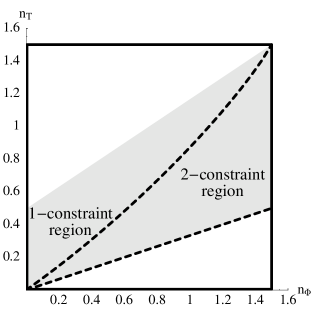
Figure 1: The shaded region is the pure-state region in the $n_{\Phi}$-$n_{T}$ plane for $4\times N$ pure states. The dashed lines are the monotone boundaries given by Eq. (8) and by $n_{T}=n_{\Phi}/3$. In the $2$-constraint region between the monotone boundaries, we set $\widetilde{H}_{\uparrow}({\bf n})=\widetilde{H}({\bf n})$, and in the 1-constraint region above the upper monotone boundary, we set $\widetilde{H}_{\uparrow}({\bf n})=\widetilde{H}(n_{T})$.

To find the doubly constrained bound on the EOF, we start with the function (2), specialized to our two constraints,

$$\widetilde{H}(n_{\Phi},n_{T})\!\! \equiv \!\!\min_{\bm{\mu}}\bigg{\{}H(\bm{\mu})\bigg{|}\sum_{j}\sqrt{\mu_{j}}=\sqrt{2n_{T}+1},$$ (7)

$$\hskip 19.91684pt3\sqrt{(\mu_{1}+\mu_{4})(\mu_{2}+\mu_{3})}=n_{\Phi}\bigg{\}}\;.\quad$$

It turns out that $\widetilde{H}(n_{\Phi},n_{T})$ is not monotonic, so we must replace it with the monotonic function $\widetilde{H}_{\uparrow}(n_{\Phi},n_{T})$ discussed above. The procedure for constructing $\widetilde{H}_{\uparrow}(n_{\Phi},n_{T})$, depicted in Fig. 1, makes a connection to the singly constrained bounds. This connection is based on the fact that the minimum of any function subject to two constraints is greater than or equal to the minimum of the same function subject to only one of the two constraints. Thus we can say that $\widetilde{H}(n_{\Phi},n_{T})\geq\widetilde{H}(n_{T})$ for all $n_{\Phi}$ and $\widetilde{H}(n_{\Phi},n_{T})\geq\widetilde{H}(n_{\Phi})$ for all $n_{T}$.

The minimum of $H(\bm{\mu})$ subject only to the $n_{T}$ constraint, i.e., $\widetilde{H}(n_{T})$, occurs when the Schmidt coefficients are given by $\bm{\mu}=(\gamma,\gamma^{\prime},\gamma^{\prime},\gamma^{\prime})$ Chen et al. (2005) with $\gamma^{\prime}=(1-\gamma)/3$. This corresponds to $n_{\Phi}=\sqrt{2(2\gamma+1)(1-\gamma)}$, thus defining a curve in the $n_{\Phi}$-$n_{T}$ plane. Writing $\gamma$ in terms of $n_{T}$ puts this curve in the form

$$n_{T}\!=\!\frac{3}{4}\!\!\left(\!1\!-\!\sqrt{1-\frac{4}{9}n_{\Phi}^{2}}\!+\!\sqrt{\frac{4}{3}n_{\Phi}^{2}\!+\!2\sqrt{\!1\!-\!\frac{4}{9}n_{\Phi}^{2}}\!-\!2}\,\right)\;.$$ (8)

Along this curve, which we call a monotone boundary, the $n_{\Phi}$ constraint is automatically satisfied when $H(\bm{\mu})$ is minimized with respect just to the $n_{T}$ constraint, which means that $\widetilde{H}(n_{\Phi},n_{T})=\widetilde{H}(n_{T})$ on this monotone boundary. To construct the required monotonic function, we set $\widetilde{H}_{\uparrow}(n_{\Phi},n_{T})=\widetilde{H}(n_{T})$ when $n_{\Phi}\leq\sqrt{2(2\gamma+1)(1-\gamma)}$, i.e., above this monotone boundary.

Similarly, the minimum of $H(\bm{\mu})$ subject just to the $n_{\Phi}$ constraint, i.e., $\widetilde{H}(n_{\Phi})$, occurs when $\bm{\mu}_{\Phi}=(\alpha,1-\alpha,0,0)$, which gives a lower monotone boundary $n_{T}=\sqrt{\alpha(1-\alpha)}=n_{\Phi}/3$. Along this line, the $n_{T}$ constraint is automatically satisfied when $H(\bm{\mu})$ is minimized with respect just to the $n_{\Phi}$ constraint, which gives $\widetilde{H}(n_{\Phi},n_{T})=\widetilde{H}(n_{\Phi})$ on this boundary. Since this lower monotone boundary coincides with the lower boundary of the pure-state region, it has no impact on defining $\widetilde{H}_{\uparrow}(n_{\Phi},n_{T})$.

The definition of $\widetilde{H}_{\uparrow}({\bf n})$ is depicted in Fig. 1. Between the monotone boundaries, a region we call the $2$-constraint region, we set $\widetilde{H}_{\uparrow}({\bf n})=\widetilde{H}({\bf n})$, and in the pure-state region above the upper monotone boundary, which we call the $1$-constraint region, we set $\widetilde{H}_{\uparrow}({\bf n})=\widetilde{H}(n_{T})$. The resulting function $\widetilde{H}_{\uparrow}({\bf n})$ is monotonic throughout the pure-state region.

We now focus on finding $\widetilde{H}({\bf n})$ in the $2$-constraint region. The method of Lagrange multipliers is not suitable for finding the minimum (7) because the problem is overconstrained. The equations obtained using Lagrange multipliers have a consistent solution only if $n_{\Phi}$ and $n_{T}$ are related as in Eq. (8), in which case $\widetilde{H}({\bf n})=\widetilde{H}(n_{T})$. This does not mean that there is no minimum for $H(\bm{\mu})$ for other values of $n_{\Phi}$ and $n_{T}$, just that the minimum lies on a boundary of allowed values of $\bm{\mu}$. The boundary with three of the Schmidt coefficients being zero is the origin in the $n_{\Phi}$-$n_{T}$ plane, where $H(\bm{\mu})=0$. The boundary with two zero Schmidt coefficients is the line $n_{T}=n_{\Phi}/3$, and along this line $\widetilde{H}({\bf n})=\widetilde{H}(n_{\Phi})$.

The minimum of $H(\bm{\mu})$ in the remaining part of the $2$-constraint region can be found using a straightforward numerical procedure. As discussed above, the constraint equations can be solved to express $\mu_{1}$, $\mu_{2}$, and $\mu_{3}$ in terms of $n_{\Phi}$, $n_{T}$, and $\mu_{4}$. There are two distinct solutions, $\bm{\mu}^{(1)}$ and $\bm{\mu}^{(2)}$. For a particular value of $\mu_{4}$, one or both of these solutions can be invalid in parts of the pure-state region because one or more of the three Schmidt coefficients lies outside the interval $[0,1]$. For valid solutions we compute the entropy $H(\bm{\mu})$.

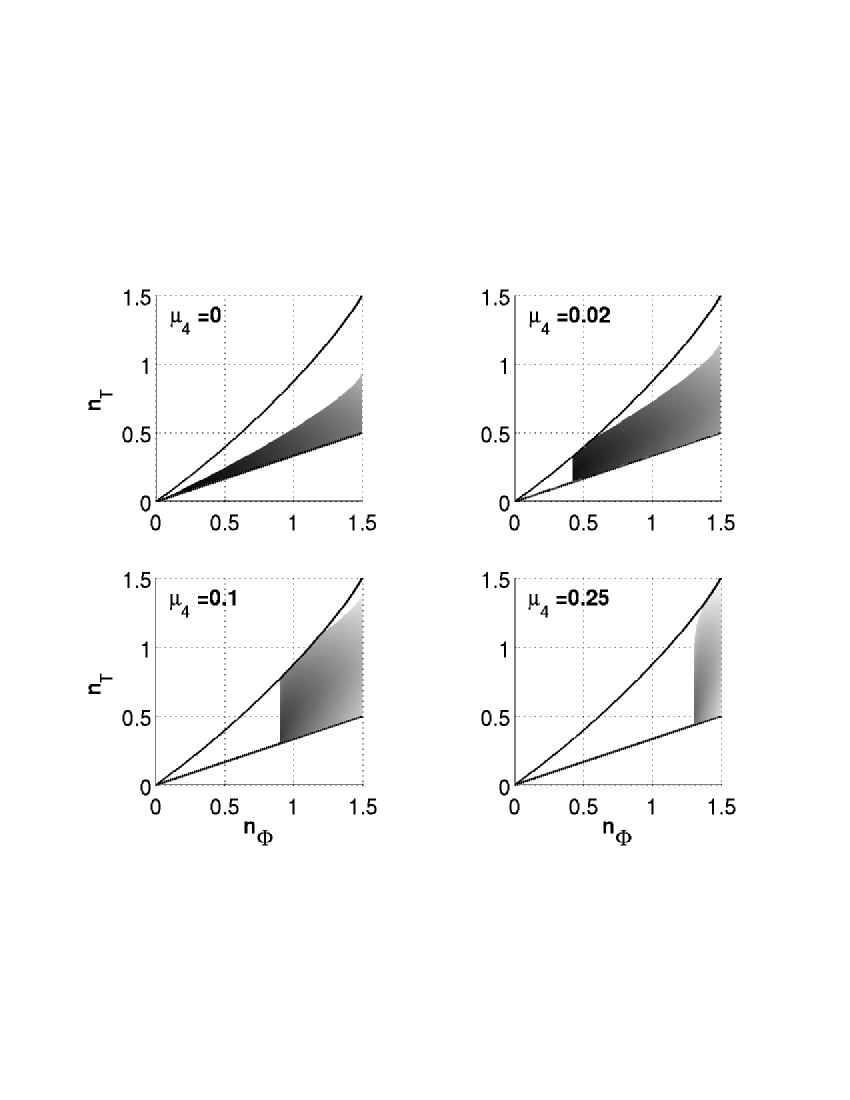
Figure 2: The part of the $2$-constraint region covered by four values of $\mu_{4}$. The two lines are the monotone boundaries.

We first consider the boundary where one Schmidt coefficient is zero by setting $\mu_{4}=0$ in the solutions $\bm{\mu}^{(1)}$ and $\bm{\mu}^{(2)}$. Not all points in the $2$-constraint region can be reached if we set $\mu_{4}=0$. This is easily seen by noticing that the point $n_{\Phi}=n_{T}=3/2$ corresponds uniquely to a maximally entangled $4\times N$ state, and for this state all four Schmidt coefficients have the value $1/4$. Indeed, a continuum of points cannot be reached if we stay on the boundary defined by $\mu_{4}=0$, so we increase the value of $\mu_{4}$ in small steps. The parts of the $2$-constraint region that are covered by four values of $\mu_{4}$ are shown in Fig. 2.

This numerical procedure gives us, for each point ${\bf n}=(n_{\Phi},n_{T})$ in the pure-state region, the range of values of $\mu_{4}$ for which $H\big{(}\bm{\mu}^{(1)}\big{)}$ and/or $H\big{(}\bm{\mu}^{(2)}\big{)}$ can be calculated at that point. The minimum of these entropies over the allowed range of values for $\mu_{4}$ is the value of $\widetilde{H}({\bf n})$.

The function $\widetilde{H}({\bf n})$ in the $2$-constraint region is, as required, a monotonic function of both $n_{\Phi}$ and $n_{T}$. It is extended to the monotonic function $\widetilde{H}_{\uparrow}({\bf n})$ on the the entire pure-state region using the procedure outlined above. The monotonic function $\widetilde{H}_{\uparrow}({\bf n})$ is not convex, however, so we must compute its convex hull ${\mathcal{H}}({\bf n})$. This can be done numerically, and it turns out that the difference between ${\mathcal{H}}({\bf n})$ and $\widetilde{H}_{\uparrow}({\bf n})$ is quite small ($\sim 10^{-3}$), the two functions differing only in a small area near the maximally entangled state. Had the pure-state region, on which $\widetilde{H}_{\uparrow}({\bf n})$ is defined, not been convex, ${\mathcal{H}}({\bf n})$ would be defined on an extended convex domain Datta et al. (2006).

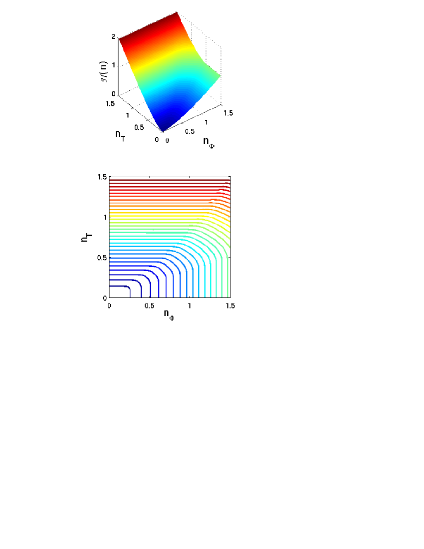
Figure 3: (Color online) The doubly constrained bound ${\mathcal{H}}({\bf n})$ on the EOF of $4\times N$ states. Also shown is a contour plot of the same function.

To obtain a bound on the EOF of all $4\times N$ states, we have to extend ${\mathcal{H}}({\bf n})$ outside the pure-state region to the rest of the $n_{\Phi}$-$n_{T}$ plane. The extension has to preserve the monotonicity of ${\mathcal{H}}({\bf n})$ so that the string of inequalities in Eq. (3) holds. This is achieved by extending ${\mathcal{H}}({\bf n})$ using surfaces that match the function at the lower and upper boundaries of the pure-state region. To preserve monotonicity, the surface added in the region below the lower boundary has zero slope along the $n_{T}$ direction, and the surface added in the region above the upper boundary has zero slope along the $n_{\Phi}$ direction. The resulting doubly constrained bound ${\mathcal{H}}({\bf n})$ on the EOF is shown in Fig. 3. The figure indicates that the extension to the whole $n_{\Phi}$-$n_{T}$ plane produces a smooth and seamless surface.

A third constraint based on the realignment criterion Rudolph (2002); Chen and Wu (2003) can be used to improve our bound on the EOF for certain classes of states. We can define the realignment negativity for a bipartite density operator $\rho$ as $n_{R}=(||{\mathcal{R}}(\rho)||-1)/2$, where $\left[{\mathcal{R}}(\rho)\right]_{ij,kl}=\rho_{ik,jl}$. For pure states, $n_{R}=n_{T}$. This means that in deriving the bounds, we could have redefined $n_{T}$ as $\max(n_{T},n_{R})$.

In this Letter we focused on the derivation of a particular doubly constrained bound on the EOF of $4\times N$ systems. Starting from the $\Phi$-map introduced by Breuer Breuer (2006a, b), we defined an entanglement monotone, the $\Phi$-negativity, and combined it with the usual negativity to formulate a doubly constrained bound. We found that the pure-state region in the $n_{\Phi}$-$n_{T}$ plane is divided into sectors by monotone boundaries. The doubly constrained pure-state marginal entropy is applicable only in the region between the monotone boundaries. In the remaining portions of pure-state region, singly constrained entropies are applicable. Monotonicity and convexity dictate how to extend the bound to all states. We expect these features to persist for systems that are not $4\times N$ and for more than two constraints, in which case the monotone boundaries will generally be hypersurfaces. A sector in which an $m$-constrained marginal entropy holds will be bounded by sectors in which $(m-1)$-constrained marginal entropies hold. These methods might provide a useful procedure for bounding the EOF and other convex-roof entanglement monotones.

This work was supported in part by Office of Naval Research grant No. N00014-03-1-0426.

References

- Bruß (2002) D. Bruß, J. Mat. Phys. 43, 4237 (2002).
- Schrödinger (1935) E. Schrödinger, Proc. Camb. Phil. Soc 31, 555 (1935).
- Einstein et al. (1935) A. Einstein, B. Podolsky, and N. Rosen, Phys. Rev. 47, 777 (1935).
- Vidal et al. (2003) G. Vidal, J. I. Latorre, E. Rico, and A. Kitaev, Phys. Rev. Lett. 90, 227902 (2003).
- Osborne and Neilsen (2002) T. Osborne and M. A. Neilsen, Quant. Inform. Process. 1, 45 (2002).
- Osterloh et al. (2002) A. Osterloh, L. Amico, G. Falci, and R. Fazio, Nature 416, 608 (2002).
- Ghosh et al. (2003) S. Ghosh, T. F. Rosenbaum, G. Aeppli, and S. N. Coppersmith, Nature 425, 48 (2003).
- Choi (1972) M. D. Choi, Can. J. Math. 24, 520 (1972).
- Plenio and Virmani (2005) M. Plenio and S. Virmani, quant-ph/0504163 (2005).
- Vidal and Werner (2002) G. Vidal and R. F. Werner, Phys. Rev. A. 65, 032314 (2002).
- Chen et al. (2005) K. Chen, S. Albeverio, and S.-M. Fei, Phys. Rev. Lett. 95, 210501 (2005).
- Terhal and Vollbrecht (2000) B. M. Terhal and K. G. H. Vollbrecht, Phys. Rev. Lett. 85, 2625 (2000).
- Datta et al. (2006) A. Datta, S. Flammia, A. Shaji, and C. M. Caves (2006), in preparation.
- Peres (1996) A. Peres, Phys. Rev. Lett. 77, 1413 (1996).
- Breuer (2006a) H.-P. Breuer, quant-ph/0605036 (2006a).
- Rudolph (2002) O. Rudolph, quant-ph/0202121 (2002).
- Chen and Wu (2003) K. Chen and L. A. Wu, Quant. Inf. Comput. 3, 193 (2003).
- Breuer (2006b) H.-P. Breuer, quant-ph/0606185 (2006b).