Quantum metrology at the Heisenberg limit with ion traps

Abstract

Sub-Planck phase-space structures in the Wigner function of the motional degree of freedom of a trapped ion can be used to perform weak force measurements with Heisenberg-limited sensitivity. We propose methods to engineer the Hamiltonian of the trapped ion to generate states with such small scale structures, and we show how to use them in quantum metrology applications.

I Introduction

The determination of small parameters has recently acquired a substantial improvement through quantum measurement, as it is now known that using probes prepared in judiciously chosen quantum states can increase their sensitivity to perturbations. As a consequence, quantum metrology has become a subject of great practical interest Giovannetti2004 . The estimation of an unknown parameter of a quantum system typically involves a three-step process: the initial preparation of a probe in a known quantum state, the interaction between the probe and the system to be measured, and a final read-out stage, where the state of the probe is determined. Typical situations are those when the system imprints an unknown parameter $x$ onto the probe through a unitary perturbation $\hat{U}_{x}=\exp(-i\,x\,\hat{G})$, where the generator $\hat{G}$ is a known Hermitian operator. The unknown small parameter $x$ of the system can be inferred by comparing the input and output states of the probe. This framework captures two important tasks in quantum metrology: i) high precision phase measurements $x=\theta$, where $\hat{U}_{\theta}$ generates a rotation in phase space of the quantum state of the probe around the origin, and ii) detection of weak forces that induce a linear displacement $x=s$ of the quantum state of the probe in some direction of phase space.

The accuracy of the parameter estimation is limited by the physical resources involved in the measurement. Techniques involving probes prepared in quasiclassical states, such as coherent states of light, have sensitivities at the standard quantum limit (SQL), also known as the shot-noise limit in the phase detection situations. Indeed, in the usual dimensionless phase-space used in quantum optics the Wigner distribution of a coherent state, with $\overline{n}$ mean number of photons, is centered at a distance $\simeq\sqrt{\bar{n}}$ from the origin, with a width $1/2$. Thus, the associated input and output states are distinguishable (approximately orthogonal) when their respective phase-space distributions are displaced by a minimal distance $1/2\simeq{\cal O}(\overline{n}^{0})$ from one another, i.e., the SQL for weak displacement measurement does not depend on the number $\overline{n}$ of photons involved in the measurement. For phase detection the smallest noticeable rotation occurs when the centers of the phase-space distributions of the input and output states have an angular distance $(1/2)/\sqrt{\bar{n}}$ measured from the origin, i.e., the SQL for phase measurement scales as $1/\sqrt{\bar{n}}$.

Using the same physical resources in addition to quantum effects, such as entanglement or squeezing, sub SQL precision can be achieved Caves1981 ; Yurke1986 ; Holland1993 ; Bollinger1996 ; Sanders1995 ; Munro2002 ; Pezze2006 . For example, probes prepared in quantum superpositions of, say, coherent states of light, have Wigner distributions with sub-Planck phase-space structures of typical linear size $1/\sqrt{\overline{n}}$ Zurek2001 . It was recently shown Toscano2006 how these structures can be used to achieve Heisenberg-limited sensitivity in weak force and phase measurements: the approximate orthogonality that allows to distinguish the input and output quantum states of the probe occurs when the peaks (valleys) of the sub-Planck structures of one come on top of the valleys (peaks) of the sub-Planck structures of the other. The minimal linear displacement required for this destructive interference is $\simeq 1/\sqrt{\overline{n}}$, defining the so-called Heisenberg limit (HL) for weak force detection. For rotations the sub-Planck phase-space structures of the Wigner function of the input state have to be at a typical distance $\simeq\sqrt{\overline{n}}$ from the origin, thus the minimal rotation angle is $\simeq 1/\overline{n}$, that defines the HL scale for phase detection. Hence, the linear size of the sub-Planck structures sets the sensitivity limit on a probe and states that saturate the limit on the smallest phase-space structures can allow one to attain Heisenberg-limited sensitivity. Sub SQL sensitivities, approaching the ultimate Heisenberg limit, have been recently achieved experimentally using multi-qubit states formed by entangled internal degrees of freedom of photons (polarization entanglement) Zeilinger2004 ; Steinberg2004 ; Zhao2004 ; Eisenberg2005 , and of trapped ions (spin entanglement) Sackett2000 ; Meyer2001 ; Liebfried2004 .

Sub-SQL precision measurements can also be achieved with continuous variables, such as the amplitude/phase of a photon trapped in a QED cavity, or the center of mass motion of trapped ions Gilchrist2004 . Such spatial modes, that can be approximately described as harmonic oscillators, can be prepared in nonclassical quantum states, e.g. superpositions of $M$ coherent states, that possess sub-Planck phase-space structures. In Toscano2006 it was shown how to use them for Heisenberg-limited precision measurements of weak forces and phase measurement, by entangling the oscillator with a two-level system. It was also proposed a concrete implementation of this strategy in the context of cavity QED (that can be extrapolated to trapped ions): a two-level atom gets entangled with the cavity mode through the (resonant or non-resonant) Jaynes-Cummings interaction in such a way that, when the atom reaches the center of the cavity, the photon field is a quantum superposition of two coherent states ($M=2$). Such “cat state” has sub-Planck oscillations parallel to the line joining the two coherent states, and is therefore Heisenberg-limited sensitive to perturbations that induce displacements that are perpendicular to that line. After the perturbation is applied, the Jaynes-Cummings evolution is undone, and the populations of the two-level atom are measured once it leaves the cavity. This provides information about the perturbation, that can be estimated with HL precision. An analysis of the decoherence processes Toscano2006 that may affect this scheme shows that this proposal should be within reach of cavity QED and ion trap experiments.

One disadvantage of the $M=2$ states is that their sensitivity gradually degrades as the direction of the perturbing force moves away from the direction orthogonal to the line joining the two coherent states. Higher order ($M>2$) superpositions of coherent states on a circle do not suffer from these limitations. In the context of cavity QED, there have been a number of schemes proposed to generate such states. In some of these proposals Brune1992 ; Parkins1993 ; Garraway1994 ; Szabo1996 ; Guo1996 it is necessary to send a sequence of atoms through the cavity and perform conditional measurements (post-selection), limiting the probability of succeeding in engineering the cavity in the desired coherent state superpositions. There are also schemes that involve only one atom, and make use of a single-atom interferometric method Domokos1994 , or a dispersive interaction between the atom and the cavity field Zeng1998-1 . The first scheme has the disadvantage of requiring post-selection, while the second one needs very long interaction times. Similar strategies have been proposed in the literature in the context of trapped ions Zeng1998-2 ; Jose2000 .

In this paper we propose ways for deterministic generation of higher order ($M>2$) coherent state superpositions with trapped ions, and how to use them to measure weak forces at the Heisenberg limit. These states do not suffer from the limitations of the $M=2$ states generated via the linear Jaynes-Cummings interactions, as discussed above. In particular, we will concentrate on how to prepare probes with $M=4$ (“compass state”) Zurek2001 and how to use them to measure small displacements (weak force detection). Our setups can also be used to measure small rotations in phase space (phase detection) by simply adding an appropriate displacement before the application of the perturbation, as described in Toscano2006 .

The paper is organized as follows. In Section II we discuss the sensitivity to perturbations of the $M=4$ compass state and we review the strategy for weak force measurements. In Section III we review the engineering of the ion-laser interaction for a single trapped ion. Section IV contains two possible approaches for generating compass states: the first one uses conditional quantum gates between the internal and the motional degrees of freedom of the ion, and the second one uses a nonlinear ion-laser engineered interaction. In Section V we implement the scheme for measuring weak forces with Heisenberg-limited sensitivity. Finally, Section VI summarizes our central results.

II Heisenberg-limited quantum metrology with continuous variables

In this section we review how to perform continuous variable based quantum metrology at the Heisenberg limit by using sub-Planck phase-space structures present in circular coherent states of a harmonic oscillator (the probe) Toscano2006 . In the following we will focus on perturbations that induce a small phase-space linear displacement of the quantum state of the probe, for example when a small force is exerted onto the probe. The unitary operator describing such a displacement is $\hat{D}(\beta)=e^{\beta\hat{a}^{\dagger}-\beta^{*}\hat{a}}$, where $\beta$ is an arbitrary small displacement in phase-space with a magnitude $|\beta|\ll|\alpha|$. In this approximation the unitary operation $\hat{D}(\beta)$ takes any coherent state $|\alpha\rangle$ to $e^{i{\rm Im}(\beta\alpha^{*})}|\alpha+\beta\rangle\approx e^{2i{\rm Im}(\beta\alpha^{*})}|\alpha\rangle$. Perturbations inducing small rotations $\hat{R}(\theta)=e^{i\theta\hat{a}^{\dagger}\hat{a}}(\theta\ll 1)$ in phase space can be treated in a similar way, as described in Toscano2006 .

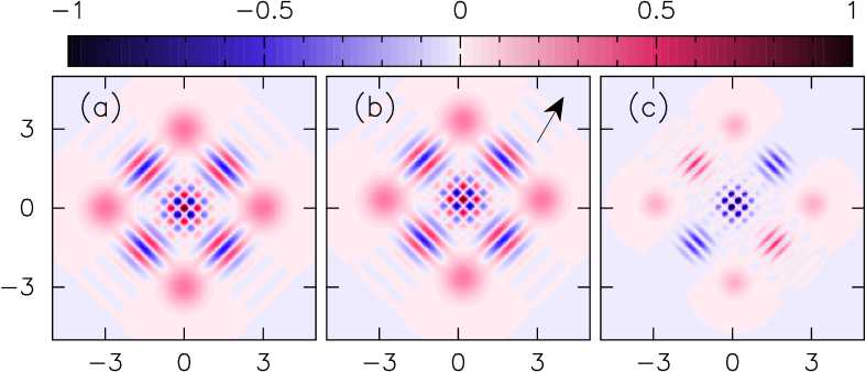
Figure 1: (Color) The Wigner functions in the $\alpha$ plane for: (a) the compass state $|\mbox{cat}_{4}\rangle$ with $\alpha=3$, and (b) the displaced compass state $\hat{D}(\beta)|\mbox{cat}_{4}\rangle=|\mbox{cat}_{4}(s_{o})\rangle$ where $\beta=e^{i\varphi}s_{o}\alpha/|\alpha|$ is a displacement of magnitude $|\beta|=s_{o}=\pi/2\,b_{+}(\varphi)|\alpha|$ in the direction relative to $\alpha$ given by $\varphi=\pi/3$. Here $b_{+}(\varphi)=\cos(\varphi)+\sin(\varphi)$. The black arrow in (b) indicates the direction of the displacement $\beta$. In (c) we display the product of the unpertubed and the perturbed Wigner functions. When performing the integration over the $\alpha$ plane of this product of Wigner functions, that is equal to the overlap $|\langle\mbox{cat}_{4}|\mbox{cat}_{4}(s_{o})\rangle|^{2}$, the negative contributions (in blue) cancel the positive ones (in red), leading to quasiorthogonality.

Circular coherent states are a special kind of states of harmonic oscillators, formed by the superposition of $M$ coherent states equidistantly placed on a circle $\cal{C}$ of radius $|\alpha|$. They are defined as

$$|{\rm cat}_{M}\rangle=\frac{{\cal N}}{\sqrt{M}}\sum_{k=1}^{M}e^{i\gamma_{k}}\;|e^{i\varphi_{k}}\alpha\rangle,$$ (1)

where $\varphi_{k}=2\pi k/M$, $\gamma_{k}$ are arbitrary phases, and ${\cal N}=1+{\cal O}(e^{-|\alpha|^{2}})$ is a normalization constant. When $|\alpha|\gtrsim 3$, it is a good approximation to take ${\cal N}=1$, and we will assume this is the case in the following considerations. These non-classical states of a harmonic oscillator have a mean number of excitations $\bar{n}\equiv\langle{\rm cat}_{M}|\hat{a}^{\dagger}\hat{a}|{\rm cat}_{M}\rangle\approx|\alpha|^{2}$. Examples of these states are the Schrödinger cat state ($M=2$), considered in detail in Toscano2006 for weak force and phase measurements, and the compass state

$$|\mbox{cat}_{4}\rangle\equiv\frac{1}{2}\left(e^{i\gamma_{1}}|i\alpha\rangle+e^{i\gamma_{2}}|-\alpha\rangle+e^{i\gamma_{3}}|-i\alpha\rangle+e^{i\gamma_{4}}|\alpha\rangle\right),$$ (2)

that we consider here.

Figure 1 depicts the Wigner function of the compass state and shows the sub-Planck phase-space structures, that oscillate with a typical wavelength $\sim 1/|\alpha|$. These structures are responsible for the Heisenberg-limited sensitivity of these states for quantum metrology applications. Indeed, the smallest linear displacement needed to distinguish the unperturbed $|\mbox{cat}_{4}\rangle$ from the perturbed $|\mbox{cat}_{4}(s)\rangle\equiv\hat{D}(\beta)|\mbox{cat}_{4}\rangle$ state of the probe (and, therefore, to attain quasi-orthogonality) is $s\sim 1/|\alpha|$, for any direction $\beta=e^{i\varphi}s\alpha/|\alpha|$. As it was shown in Toscano2006 , the sub-Planck structures of the Wigner functions of the circular states determine the oscillatory behavior of the fidelity function $f(s)\equiv|\langle\mbox{cat}_{4}|\mbox{cat}_{4}(s)\rangle|^{2}$, that for the compass state reads

$$f(s) \approx \frac{1}{16}\left|\sum_{k=1}^{4}\;e^{i{\rm Im}(\beta\alpha_{k}^{*})}\;\langle\alpha_{k}|\alpha_{k}+\beta\rangle\right|^{2}$$ (3)

$$= e^{-s^{2}}\,\cos^{2}\big{(}b_{+}(\varphi)|\alpha|s\big{)}\cos^{2}\big{(}b_{-}(\varphi)|\alpha|s\big{)},$$

where $\alpha_{k}\equiv e^{i\varphi_{k}}\alpha$ and $b_{\pm}(\varphi)\equiv\cos(\varphi)\pm\sin(\varphi)$ ($\varphi$ is the angle between $\beta$ and $\alpha$). Here we have neglected contributions $\langle\alpha_{l}|\alpha_{k}+\beta\rangle\approx{\cal O}\big{(}e^{-|\alpha|^{2}}\big{)}$ for $l\neq k$, that is a good approximation for $|\alpha|\gtrsim 3$, and we have used that $\langle\alpha_{k}|\alpha_{k}+\beta\rangle=e^{-|\beta|^{2}}\exp\left\{i{\rm Im}(\beta\alpha_{k}^{*})\right\}$. When $e^{-s^{2}}\approx 1$, valid for $|\beta|=s\ll 1$, we can re-write the fidelity function as

$$f(s)\approx\cos^{2}\big{(}b_{+}(\varphi)|\alpha|s\big{)}\cos^{2}\big{(}b_{-}(\varphi)|\alpha|s\big{)}.$$ (4)

Note that $f(s)$ does not depend on the phases $\gamma_{k}$ that enter in the definition of the compass state $|\mbox{cat}_{4}\rangle$ in Eq.(2). We can see in Figure 2 the oscillatory behavior of the fidelity $f(s)$ as a function of the magnitude of the linear displacement $s=|\beta|$ with a typical wavelength $\sim 1/|\alpha|$. The minimal displacement to achieve quasi-orthogonality, $s_{o}$, can be obtained equating to zero the approximation in Eq.(4) because we see in Fig.2 that this approximation well describes the fidelity beyond $s_{o}$. Thus, the minimal displacement to achieve quasi-orthogonality is approximately given by

$$s_{o}\approx\frac{\pi}{2b(\varphi)|\alpha|},$$ (5)

where $b(\varphi)\equiv\mbox{max}\{|b_{+}(\varphi)|,|b_{-}(\varphi)|\}$ (see Fig.(2)). The scaling of $s_{o}$ as $1/|\alpha|$ implies that one can detect displacement perturbations with Heisenberg-limited sensitivity. Note that $b_{+}(\varphi)$ and $b_{-}(\varphi)$ are never simultaneously zero in the interval $[0,2\pi]$, which means that for any direction of the displacement $\beta$ there is a minimum (finite) displacement for which the unperturbed and the perturbed compass states are quasi-orthogonal. Contrary to the cat state ($M=2$), whose HL sensitivity degrades as the direction of the perturbation $\beta$ tends to the direction of $\alpha$ (i.e., as $\varphi\rightarrow 0$), compass states are HL sensitive for all directions $\varphi$ of the perturbing force. In a similar way, one can show that compass states have Heisenberg-limited sensitivity to rotation perturbations, that is, the minimal rotation angle that can be detected is $\theta\simeq s/|\alpha|\simeq 1/|\alpha|^{2}$. To achieve this sensitivity for rotation perturbations, the circular coherent state has to be first translated in phase space so that the displaced circle ${\cal C}$ contains the origin of phase space Toscano2006 .

Figure 2: The fidelity $f(s)\equiv|\langle\mbox{cat}_{4}|\mbox{cat}_{4}(s)\rangle|^{2}$ as a function of the magnitude of the linear displacement $s=|\beta|$ (full line) where $\beta=e^{i\varphi}s\alpha/|\alpha|$ with $\varphi=\pi/3$. The circles $(\circ)$ correspond to points given by the approximation in Eq.(3). The dashed line is the approximation in Eq.(4) The displacement corresponding to quasiorthogonality, i.e., $s_{o}$ in Eq.(5) is indicated in the plot.

Once the direction of the perturbation $\beta$ is known, i.e., the angle $\varphi$), the information about its magnitude is encoded in the fidelity function $f(s)$ between the unperturbed and the perturbed states of the probe. In order to measure the fidelity, a measurement strategy was proposed in Toscano2006 , that is summarized in Fig. (3). It involves entangling the probe with an ancillary system, a two-level system (TLS), and designing their interaction $\hat{U}$ in such a way that the information about the overlap between the unperturbed and perturbed probes states can be inferred from measurements of the populations of the TLS. Starting with an initial joint state $|\Psi_{i}\rangle=|0\rangle\otimes|g\rangle$, where $|0\rangle$ is the vacuum state of the probe and $|g\rangle$ the lower state of the ancilla, the evolved states, with and without the perturbation applied, are $|\Phi\rangle=\hat{U}_{x}\hat{U}|\Psi_{i}\rangle$ and $|\Psi\rangle=\hat{U}|\Psi_{i}\rangle$ respectively. Here $\hat{U}_{x}$ denotes the unitary operator corresponding to the perturbation. The interaction evolution $\hat{U}$ has to be designed in such a way that $|\langle\Psi|\Phi\rangle|^{2}\approx|\langle{\rm cat}_{4}|{\rm cat}_{4}(x)\rangle|^{2}$. Then, we have to undo the unitary evolution $\hat{U}$ to obtain a final entangled state of the composite system

$$|\Psi_{f}\rangle=\sqrt{P_{e}}|e,\Psi^{e}_{S}\rangle+\sqrt{P_{g}}|g,\Psi^{g}_{S}\rangle\;\;,$$ (6)

where $P_{e}$ and $P_{g}=1-P_{e}$ are the probabilities of measuring the TLS in levels $e$ and $g$, respectively, given by

$$P_{g}=1-P_{e}=\frac{|\langle\Psi_{i}|\Psi_{f}\rangle|^{2}}{|\langle 0|\Psi^{g}_{S}\rangle|^{2}}\approx\frac{|\langle{\rm cat}_{M}|{\rm cat}_{M}(x)\rangle|^{2}}{|\langle 0|\Psi^{g}_{S}\rangle|^{2}}\;\;.$$ (7)

As mentioned in Toscano2006 , this strategy can also be used to measure the Loschmidt echo, which quantifies the sensitivity of a quantum system to perturbations. Also, similar hybrid continuous variable-qubit systems have been proposed for quantum information processing and quantum computation Lee2006 ; Spiller2006 .

Later in the paper we will show how to create compass states of the vibrational degree of freedom of a trapped ion, and how to measure weak perturbations at the Heisenberg limit by entangling the motional degree of freedom with a two-level system, corresponding to two internal hyperfine levels of the ion.

Figure 3: Circuit diagram to measure a small perturbation $\hat{U}_{x}$ at the Heisenberg limit. The probe is a harmonic oscillator and the ancilla a two-level system. The entangling evolution $\hat{U}$ is such that $|\langle\Psi|\Phi\rangle|^{2}\approx|\langle{\rm cat}_{4}|{\rm cat}_{4}(x)\rangle|^{2}$, where $|{\rm cat}_{4}\rangle$ is the compass state defined in Eq.(2), and $|{\rm cat}_{4}(x)\rangle=\hat{U}_{x}|{\rm cat}_{4}\rangle$ the perturbed compass state (see text for details).

III Engineering the ion -laser interaction in an ion trap.

Let us consider a single ion confined inside a harmonic trap. In good approximation the quantized motion of the ion center-of-mass along each spatial dimension can be described by a quantum harmonic oscillator. When the ion is illuminated by laser light quasi-resonant to one of its electronic transitions its motional degrees-of-freedom can be coupled to the electronic ones via photon-momentum exchange. The laser excitation can be done in several different ways, giving rise to a large number of possible interaction Hamiltonians between electronic and motional degrees-of-freedom. Here we will be interested in two basic types of laser excitation in a situation where the motional sidebands can be spectroscopically well resolved. Moreover, we will consider the excitation of only one motional degree-of-freedom.

The first excitation scheme of interest is the Raman excitation of a dipole-forbidden electronic transition between two hyperfine electronic states, on resonance to a given motional sideband. This can be done via the off-resonant excitation of an intermediary electronic level by two laser fields of adequate frequencies (see Fig. 4(a)). In this case, the interaction Hamiltonian, in the interaction picture, is given by vo-ma :

$$\hat{H}_{I}=\frac{1}{2}\hbar|\Omega_{0}|\,e^{i\phi}\,\hat{\sigma}_{+}\hat{f}_{k}(\hat{n},\eta)\;\hat{a}^{k}+\mbox{H.c.}\;,$$ (8)

where the operator-valued function $\hat{f}_{k}(\hat{n},\eta)$ depends on the motional number operator $\hat{n}\equiv\hat{a}^{\dagger}\hat{a}$,

$$\hat{f}_{k}(\hat{n},\eta)=e^{-\eta^{2}/2}\sum_{l=0}^{+\infty}\frac{(i\eta)^{2l+k}}{l!(l+k)!}\;\frac{\hat{n}!}{(\hat{n}-l)!}\;\;,$$ (9)

and we define $\hat{n}!/(\hat{n}-l)!\equiv[\hat{n}-(l-1)][\hat{n}-(l-2)]\ldots\hat{n}$. The operators $\hat{\sigma}_{+}$ and $\hat{a}$ are the electronic flip operator between the states $|g\rangle$ and $|e\rangle$ and the annihilation operator of a motional quantum, respectively. $\Omega_{0}=|\Omega_{0}|\,e^{i\phi}$ is the effective Raman Rabi frequency and $k$ corresponds to the excitation of the $k$th lower motional sideband (in the example of Fig. 4(a) $k\!=\!1$). The Lamb-Dicke parameter $\eta$ can be defined as $\eta=({\bf\delta k_{L}\cdot u})\Delta x_{0}$, where $\Delta x_{0}$ is the spread of the motional wave function in the ground state of the harmonic potential and $\bf u$ is a unit vector giving the direction of the motional degree-of-freedom we are considering. The vector ${\bf\delta k_{L}}={\bf k_{L_{1}}}\!-\!{\bf k_{L_{2}}}$ is the difference of the wave vectors of the two Raman lasers. The value of the Lamb-Dicke parameter $\eta$ can be changed via the geometry of the laser beams in two different ways. The first one consists in changing the modulus of the vector ${\bf\delta k}$. This modulus reaches its minimum value when the laser beams are co-propagating and its maximum value when the laser beams are counter-propagating. The second way consists in changing the direction of the vector ${\bf\delta k}$ with respect to the unit vector ${\bf u}$. So, via the laser geometry, it is possible to change the value of $\eta$ in some extent. In particular, using co-propagating laser beams, one can reach the Lamb-Dicke regime where $\eta\ll 1$.

Figure 4: Electronic (internal) and motional (external) energy levels (not to scale) of a trapped ion, coupled by two Raman lasers. (a) corresponds to the first red sideband transition between two electronic levels, and (b) corresponds to the first blue sideband transition via the virtual excitation of an electronic level.

Note that when $\eta\ll 1$ the function $\hat{f}_{k}(\hat{n},\eta)\approx(i\eta)^{k}$. In this case, the excitation of the carrier resonance ($k=0$) leads to the interaction Hamiltonian:

$$\hat{H}_{I}=\frac{1}{2}\hbar|\Omega_{0}|\,e^{i\phi}\,\hat{\sigma}_{+}+\mbox{H.c.}\;.$$ (10)

This Hamiltonian allows one to perform rotations of the electronic state of the ion according to the evolution operator

$$\hat{U}_{\theta}(\vec{v})\equiv e^{-i\hat{H}_{I}t/\hbar}=\cos\left(\frac{\theta}{2}\right)-i\sin\left(\frac{\theta}{2}\right)(v_{x}\hat{\sigma}_{x}+v_{y}\hat{\sigma}_{y})\;\;,$$ (11)

where $\theta=|\Omega_{0}|t$, $v_{x}=\cos(\phi)$, $v_{y}=-\sin(\phi)$ and $\hat{\sigma}_{x}$, $\hat{\sigma}_{y}$ are the Pauli operators. Our weak force measurement scheme involves reversing every unitary evolution applied in the process. Hence, the inverse evolution $\hat{U}_{\theta}(-\vec{v})$ can be implemented simply by changing by $\phi\rightarrow\phi+\pi$ the phase of the effective Raman Rabi frequency $\Omega_{0}$.

In situations where the value of the parameter $\eta$ is not extremely small ($\eta\approx(0.1,0.2)$) terms of order $\eta^{2}$ should be taken into account in Eq. (9). In this case, for carrier excitation ($k=0$), the function $\hat{f}_{0}(\hat{n},\eta)$ can be written as:

$$\hat{f}_{0}(\hat{n},\eta)\approx A_{0}+A_{1}\hat{n},$$ (12)

with $A_{0}=1-\eta^{2}/2$ and $A_{1}=-\eta^{2}$. Under this condition, the choice of $\phi=0$ in the Hamiltonian (8) leads to the evolution operator

$$\hat{R}_{c}(\bar{\theta})\equiv e^{-i\hat{H}_{I}t/\hbar}=e^{i\nu\hat{\sigma}_{x}}\;e^{i\bar{\theta}\hat{\sigma}_{x}\hat{n}},$$ (13)

where $\nu=-|\Omega_{0}|tA_{0}/2$ and $\bar{\theta}=-|\Omega_{0}|tA_{1}/2$. The action of this operator corresponds to a rotation in phase-space of the motional state of the ion conditioned to its electronic state:

$$\hat{R}_{c}(\bar{\theta})|\alpha\rangle|\uparrow_{x}\rangle = e^{i\nu}\;|\alpha\;e^{i\bar{\theta}}\rangle|\uparrow_{x}\rangle$$

$$\hat{R}_{c}(\bar{\theta})|\alpha\rangle|\downarrow_{x}\rangle = e^{-i\nu}\;|\alpha\;e^{-i\bar{\theta}}\rangle|\downarrow_{x}\rangle,$$ (14)

where $|\alpha\rangle$ represents a coherent motional state, $|\uparrow_{x}\rangle\equiv(|e\rangle+|g\rangle)/\sqrt{2}$ and $|\downarrow_{x}\rangle\equiv(|e\rangle-|g\rangle)/\sqrt{2}$ are eigenstates of the $\hat{\sigma}_{x}$ Pauli operator, and $|e\rangle$ and $|g\rangle$ represent, respectively, the upper and lower electronic states of the transition driven by the lasers (eigenstates of the $\hat{\sigma}_{z}$ Pauli oparator). The inverse operation $\hat{R}_{c}(-\bar{\theta})$ can be implemented choosing $\phi=\pi$.

The dependence of the Hamiltonian (8) on the motional number operator $\hat{n}$ is determined by the function $\hat{f}_{k}(\hat{n},\eta)$. Some control of this dependence is obtained by changing the value of the Lamb-Dicke parameter $\eta$. However, this control is rather limited and it is of interest to find ways of extending the possibilities of tailoring the $\hat{n}$-dependence of the Hamiltonian  (8). As has been shown in ma-vo1 , some extra tailoring can be done by exciting the same vibrational sideband of the ion by $N$ pairs of Raman lasers of arbitrary effective Rabi frequencies $\Omega_{j}$ and Lamb-Dicke parameters $\eta_{j}\,(j\!=\!1,\dots,N)$. Remember that the parameter $\eta_{j}$, corresponding to a given pair of Raman lasers, can be controlled by varying the geometry of those laser beams. Under such excitation scheme the resulting interaction Hamiltonian maintains the general form of the Hamiltonian (8). The combined effect of the $N$ laser pairs appears in the operator function $\hat{f}_{k}(\hat{n})$, which is transformed in the engineered function $\hat{f}_{k}^{\mbox{\tiny(e)}}(\hat{n})$. This function can be written in the form of a Taylor series,

$$\hat{f}_{k}^{\mbox{\tiny(e)}}(\hat{n})=\sum_{p=0}^{\infty}\,A_{p}\,\hat{n}^{p},$$ (15)

with the coefficients $A_{p}$ given by

$$A_{p}=\left\{\begin{array}[]{ccc}\displaystyle\sum_{j=1}^{N}\,e^{-\eta_{j}^{2}/2}\frac{\Omega_{j}}{\Omega_{L}}\frac{(i\eta_{j})^{k}}{k!}&\mbox{if}&p=0,\\[4.30554pt] (-1)^{p}\displaystyle\sum_{j=1}^{N}\,e^{-\eta_{j}^{2}/2}\frac{\Omega_{j}}{\Omega_{L}}{(i\eta_{j})}^{k}\alpha_{p,j}&\mbox{if}&p\neq 0,\end{array}\right.$$ (16)

where $\Omega_{L}$ is a reference Rabi frequency and the coefficients $\alpha_{p,j}$ are definded by:

$$\alpha_{p,j}=\sum_{m=p}^{\infty}\,(-1)^{m-p}S_{m}^{(p)}\frac{\eta_{j}^{2m}}{m!(m+k)!}\;.$$ (17)

The $S_{m}^{(p)}$ are the Stirling numbers of first kind abramowitz , that count the number of permutations of $m$ elements with $p$ disjoint cycles. The above expression shows that, for a given set of parameters $\eta_{j}$, $N$ of the coefficients $A_{p}$ can be independently fixed by the values of the $N$ Rabi frequencies $\Omega_{j}$. The values of the Rabi frequencies are the solutions of the set of $N$ linear equations obtained from Eq.(16) by fixing the values for the $N$ coefficients $A_{p}$. The free parameters $\eta_{j}$ can be used to optimize the coupling between the electronic and the vibrational degrees of freedom. This excitation scheme opens the possibility for engineering a large number of interaction Hamiltonians.

In the next section we will be interested in engineering the function

$$\hat{f}_{k}^{\mbox{\tiny(e)}}(\hat{n},\eta)=A_{0}+A_{1}\hat{n}+A_{2}\hat{n}^{2}+\mbox{\cal O}(\eta^{8}_{\mbox{\scriptsize max}}\hat{n}^{4}),$$ (18)

where only the values of $A_{2}$ and $A_{3}=0$ have to be fixed independently. This can be done with $N=2$ pairs of laser beams in Raman configuration. If the two laser pairs excite the carrier resonance ($k=0$), the resulting interaction Hamiltonian will be

$$\hat{H}_{I}=\frac{1}{2}\hbar|\Omega_{L}|\,e^{i\phi}\,\hat{\sigma}_{+}\hat{f}_{k}^{\mbox{\tiny(e)}}(\hat{n},\eta)+\mbox{H.c.}\;.$$ (19)

For $\phi=0$ in the above equation one gets the following Kerr-type evolution operator

$$\hat{V}(\phi_{2})\equiv e^{-i\hat{H}_{I}t/\hbar}=e^{-i\phi_{0}\hat{\sigma}_{x}}\;e^{-i\phi_{1}\hat{\sigma}_{x}\hat{n}}\;e^{-i\phi_{2}\hat{\sigma}_{x}\hat{n}^{2}}\;\;,$$ (20)

with $\phi_{j}=|\Omega_{L}|A_{j}t/2$ ($j=0,1,2$). We index $\hat{V}$ just with $\phi_{2}$ because, when applying this operation to a trapped ion, only the value taken by $\phi_{2}$ will be of importance. Note that the evolution generated by $\hat{V}(\phi_{2})$ may be inverted by setting $\phi=\pi$ in Eq.(19).

The second basic type of laser excitation scheme we are interested in is the Raman excitation of one motional sideband via the virtual excitation of a given electronic transition (see Fig. (4(b)). In this excitation scheme only the motional degree-of-freedom is excited conditioned on the occupation of a specific electronic level. In the example of Fig. (4(b)), if the ion is in the electronic state $|g\rangle$ nothing happens, whereas if the ion is in the electronic state $|e\rangle$ its vibrational motion will be excited. In this case the interaction Hamiltonian, describing the action of the lasers on the motional degree-of-freedom, is given by wal-vo ; Monroe1996

$$\hat{H}_{I}=\frac{1}{2}\hbar|\Omega_{0}|\,e^{i\phi}\hat{f}_{k}(\hat{n},\eta)\;\hat{a}^{k}+\mbox{H.c.}\;.$$ (21)

When the first motional sideband is excited ($k=1$) in a situation where $\eta\ll 1$, the above Hamiltonian simplifies to

$$\hat{H}_{I}=\frac{1}{2}\hbar|\Omega_{0}|\,e^{i\phi}\hat{a}+\mbox{H.c.}\;.$$ (22)

The time-evolution generated by the Hamiltonian (22) is equivalent to action of the displacement operator $\hat{D}(\alpha)$

$$\hat{U}(t)\equiv e^{-i\hat{H}_{I}t/\hbar}=\hat{D}\left(-\frac{1}{2}\eta|\Omega_{0}|\,e^{-i\phi}t\right).$$ (23)

For this reason, the Hamiltonian (22) can be used to coherently displace the motional state of the ion in phase-space conditioned on the occupation of a given electronic level. In order to stress the dependence of the action of the above Hamiltonian on the electronic state we will represent the evolution operator (23) by $\hat{D}_{c}(\alpha)$.

IV Dynamical generation of the compass state in ion traps

According to the general procedure to measure small perturbations, summarized in Fig.(3), the measurement of weak forces that couple to the motional degree of freedom of a trapped ion involves the dynamical generation of an intermediate maximally entangled state between the electronic (the ancilla) and the motional (the probe) degree of freedom of the ion, i.e.,

$$|\Psi\rangle=\frac{1}{\sqrt{2}}\;\;|\mbox{cat}_{4}\rangle\;|\uparrow\rangle\;+\frac{1}{\sqrt{2}}\;\;|\overline{\mbox{cat}_{4}}\rangle\;|\downarrow\rangle\;\;,$$ (24)

where $|\uparrow\rangle$, $|\downarrow\rangle$ are two orthogonal internal states of the ion, and $|\mbox{cat}_{4}\rangle$, $|\overline{\mbox{cat}}_{4}\rangle$ are compass states (Eq.(2)) of the center-of-mass motion of the ion. In the following we describe two ways to dynamically generate these states starting from an initial state of the form $|\Psi_{f}\rangle=|0\rangle\otimes|g\rangle$, where $|0\rangle$ is the ground state of the center-of-mass motion of the ion and $|g\rangle$ is the lower electronic state considered. The first approach combines quantum gates over the internal states and conditional linear operations over the center-of-mass motion, described in Section III. The second approach uses the engineering of a non-linear ion-laser interaction of the Kerr-type, also described in Section III.

IV.1 First approach

Figure 5: Circuit diagram to generate the compass state via quantum gates. Starting with an initial state $|\Psi_{i}\rangle=|0\rangle\otimes|g\rangle$ of a trapped ion, where $|0\rangle$ is the ground state of its center-of-mass motion, and $|g\rangle$ is the lowest of the two hyperfine electronic states considered, this sequence of unitary operations generates an output state $|\Psi\rangle$ of the form in Eq.(24), with $|\uparrow\rangle\equiv|e\rangle$ and $|\downarrow\rangle\equiv|g\rangle$, and $|\mbox{cat}_{4}\rangle$ and $|\overline{\mbox{cat}}_{4}\rangle$ compass states. The unitary evolution $\hat{U}$ in Fig.(3) is composed of this sequence of operations.

In this approach the set of unitary operations that leads to the state in Eq.(24) is described in Fig. 5. The first type of unitary operations in the sequence are the quantum gates $\hat{U}_{\theta}(\vec{v})$, given by the carrier $\theta$-pulses in Eq.(11) that rotate the internal states of the ion around the Bloch vector $\vec{v}$ by an angle $\theta$. We only perform rotations around the Bloch vector $\vec{v}=(0,v_{y},0)$ that can be carried out by choosing the phase of the effective Raman Rabi frequency $\Omega_{0}$ equal $\phi=-\pi/2$. Setting the time duration of the pulse $\theta=\pi/2=|\Omega_{0}|t_{\pi/2}$ we can implement $\hat{U}_{\pi/2}(v_{y})$, that performs $\pi/2$-rotations, and with $\theta=\pi=|\Omega_{0}|t_{\pi}$ we implement $\hat{U}_{\pi/2}(v_{y})$, that performs $\pi$-rotations. The other type of unitary operations in the sequence of Fig.5 affect the motional state of the ion conditioned on the state of the electronic degree of freedom. $\hat{D}_{c}(\bar{\alpha})$ given in Eq.(23) displaces a coherent state of the vibrational motion of the ion if the internal electronic part is in the upper state $|e\rangle$, and does nothing if the electronic part is in the ground state. That is, $\hat{D}_{c}(\bar{\alpha})|\alpha\rangle|e\rangle=e^{i{\rm Im}(\bar{\alpha}\alpha^{*})}|\alpha+\bar{\alpha}\rangle|e\rangle$, and $\hat{D}_{c}(\bar{\alpha})|\alpha\rangle|g\rangle=|\alpha\rangle|g\rangle$. The conditioned operation $\hat{R}_{c}(\pi/4)$ in Fig. 5 performs phase space rotations of a coherent state of the vibrational motion of the ion according to Eq.(III).

The final entangled state $|\Psi\rangle$ of the sequence of unitary operations of Fig. 5 is of the form given in Eq.(24), with $|\uparrow\rangle=|e\rangle$ and $|\downarrow\rangle=|g\rangle$, and the vibrational motion of the ion in compass states of the form

$$|\mbox{cat}_{4}\rangle = \frac{1}{2}\left(e^{i\nu}|i\alpha\rangle+e^{-i\nu}|-\alpha\rangle-e^{i\nu}|-i\alpha\rangle+e^{-i\nu}|\alpha\rangle\right),$$

$$|\overline{\mbox{cat}}_{4}\rangle = \frac{1}{2}\left(e^{i\nu}|i\alpha\rangle-e^{-i\nu}|-\alpha\rangle-e^{i\nu}|-i\alpha\rangle-e^{-i\nu}|\alpha\rangle\right),$$

that are equally oriented in phase space.

A realistic estimation for the total time needed to perform the unitary operations in this approach can be done using the experimental parameters in Monroe1996 . For the $\hat{U}_{\pi/2}(v_{y})$ operation the Raman Rabi frequency is of the order $\Omega_{0}/2\pi\approx 250$ kHz, so the $\pi$-pulse duration is about $1\mu$s. This implies a total time for single qubit operations of about $2.5\mu$s. The conditional displacement $\hat{D}_{c}(\bar{\alpha})$ of amplitude $|\bar{\alpha}|=\eta\Omega_{0}\tau/2$ can be implemented with a Lamb-Dicke parameter $\eta\approx 0.15$ and an effective strength of the Raman laser configuration $\Omega_{0}/2\pi\approx 300$kHz. Let us suppose that we create compass states with amplitude $|\alpha|\approx 3$, thus for the maximum displacement in the process $\bar{\alpha}=2\alpha$ we have a duration time $\tau\approx 21\mu$s. Therefore, the total time for the conditional displacements in the process is aproximately $42\mu$s. For the duration of the conditional rotation $\hat{R}_{c}(\bar{\theta})$ we have $\bar{\theta}=\pi/4=\Omega_{0}\eta^{2}t_{\pi/4}/2$, and using also $\eta\approx 0.15$ and $\Omega_{0}/2\pi\approx 300$kHz, we get $t_{\pi/4}\approx 27\mu$s. Hence, the total time needed to generate the state $|\Psi\rangle$ is approximately $72\mu$s.

IV.2 Second approach

Figure 6: Circuit diagram to generate the compass state via engineered Kerr nonlinearity $\hat{V}$. The input state is the same as in Fig. 5. The output state $|\Psi\rangle$ has the form in Eq.(24), with $|\uparrow\rangle\equiv|\uparrow_{x}\rangle$ and $|\downarrow\rangle\equiv|\downarrow_{x}\rangle$, and $|\mbox{cat}_{4}\rangle$ and $|\overline{\mbox{cat}}_{4}\rangle$ compass states. The unitary evolution $\hat{U}$ in Fig.(3) is composed of this sequence of operations.

In this approach the set of unitary operations that leads to the state in Eq.(24) is described in Fig. 6. The displacement operator $\hat{D}_{c}(\alpha)$ acting on the vibrational state of the ion can be implemented along the lines of Section III, where now the Raman excitation of one motional sideband is via the virtual excitation of the electronic transition with the lower state $|g\rangle$. The engineered Kerr operation $\hat{V}=e^{-i\phi_{0}\hat{\sigma}_{x}}e^{-i\phi_{1}\hat{\sigma}_{x}\hat{n}}e^{-i\phi_{2}\hat{\sigma}_{x}\hat{n}^{2}}$ generates all the circular coherent states in Eq.(1) of the vibrational degree of freedom for $\phi_{2}=\pi/M$ compass-state-generation . In particular, we can see that the compass state ($M=4$) is generated because $e^{\pm i(\pi/4)\hat{n}^{2}}|\alpha\rangle=\frac{1}{2}\left(e^{\pm i(\pi/4)}\left(|\alpha\rangle-|-\alpha\rangle\right)+\left(|i\alpha\rangle+|-i\alpha\rangle\right)\right)$. The total unitary operation is $\hat{U}=\hat{V}(\pi/4)\hat{D}_{c}(\alpha)$, and the output state $|\Psi\rangle$ is of the form given in Eq.(24), with the electronic part as $|\uparrow\rangle=|\uparrow_{x}\rangle$ and $|\downarrow\rangle=|\downarrow_{x}\rangle$, and the vibrational motion of the ion in compass states of the form

$$|\mbox{cat}_{4}\rangle = \frac{e^{-i\phi_{0}}}{2}\left[e^{-i\pi/4}\big{(}|\bar{\alpha}\rangle-|-\bar{\alpha}\rangle\big{)}+|i\bar{\alpha}\rangle+|-i\bar{\alpha}\rangle\right],$$

$$|\overline{\mbox{cat}}_{4}\rangle = -\frac{e^{i\phi_{0}}}{2}\left[e^{i\pi/4}\big{(}|\tilde{\alpha}\rangle-|-\tilde{\alpha}\rangle\big{)}+|i\tilde{\alpha}\rangle+|-i\tilde{\alpha}\rangle\right].$$

Here $\tilde{\alpha}=\alpha e^{i\phi_{1}}$, and $\bar{\alpha}=\alpha e^{-i\phi_{1}}$. These two compass states are rotated with respect to each other in an angle $2\phi_{1}$. If it is desired to have the compass states equally oriented in phase space, as in the first approach, a conditional rotation could be performed.

The engineering of the interaction Hamiltonian can be accomplished with $N=2$ pairs of Raman lasers (with Lamb-Dicke parameters $\eta_{j}$ and Rabi frequencies $\Omega_{j}$, $j=1,2$) driving resonantly the carrier ($k=0$) transition. Indeed, one can choose the coefficient of the quadratic $\hat{n}^{2}$ part in Eq.(18) to be $A_{2}=1$, and impose that the cubic coefficient identically vanishes, $A_{3}=0$. This sets the time $t^{*}$ when the compass state is generated as $\phi_{2}=|\Omega_{L}|A_{2}t^{*}/2=\pi/4$. The compass state is formed at the time $t^{*}$ irrespective of the values that the phases $\phi_{0}$ and $\phi_{1}$ take. Thus, we do not require any fixed values for $A_{0}$ and $A_{1}$ in the interaction Hamiltonian, simplifying the engineering design to only two pairs of Raman lasers. Selecting the set of Lamb-Dicke parameters $\eta_{j}$ for the two pair of lasers as $\{0.4,0.35\}$ yields for the relative Rabi frequencies $\Omega_{j}/\Omega_{L}$ the values $\{-520,1154\}$. This requires that the Rabi frequencies of the two pair of lasers be related as $|\Omega_{2}|\approx 2.2|\Omega_{1}|$, and have a $\pi$ phase shift with respect to each other. The coefficients $A_{0}$ and $A_{1}$ are dependent quantities that can be obtained from Eqs.(16,17), and are equal to $A_{0}\approx 605$ and $A_{1}\approx-57$. In order to minimize $t^{*}$ we choose the highest experimentally available Rabi frequencies, $|\Omega_{1}|\approx 5$MHz and $|\Omega_{2}|\approx 11$MHz. Therefore, the reference Rabi frequency $\Omega_{L}$ is $|\Omega_{L}|\approx 9.5\times 10^{3}{\rm s}^{-1}$, and the time $t^{*}$ at which the compass states is generated is equal to $t^{*}=\pi/2|\Omega_{L}|\approx 165\mu{\rm s}$. The total time needed to generate the final state $|\Psi\rangle$ in Fig.6 is equal to the duration of the conditional displacement (approximately equal to $10\mu{\rm s}$ for $|\alpha|\approx 3$, see previous sub section), plus the time $t^{*}$ for the compass state generation, that is a total time of approximately $175\mu{\rm s}$.

V Weak force detection scheme

Once the intermediate state of the form Eq.(24) is created, either by means of the first or second approaches, the probe is subjected to the perturbation to be measured. We are interested in weak classical forces that couple to the center-of-mass motion of the ion, and thus cause a small linear displacement of the motional quantum state of the ion, irrespective of its internal electronic state. This can be simulated by applying the displacement operator $\hat{D}_{c}(\beta=e^{i\varphi}s\alpha/|\alpha|$) on the vibrational state of the ion with two pairs of Raman lasers, each of them inducing an equal blue sideband transition on the $|g\rangle$ and $|e\rangle$ states (see Section III). Alternatively, a uniform electric field oscillating near the trap frequency results in a displacement perturbation acting equally on both $|g\rangle$ and $|e\rangle$ Myatt2000 . The general form of the created perturbed state is

$$|\Phi\rangle=\frac{1}{\sqrt{2}}\;\;|\mbox{cat}_{4}(s)\rangle\;|\uparrow\rangle\;+\frac{1}{\sqrt{2}}\;\;|\overline{\mbox{cat}_{4}(s)}\rangle\;|\downarrow\rangle\;\;.$$ (25)

After reversing the evolution along the lines described in Sections III and IV we get the final entangled state of the form in Eq.(6). In the first approach we have

$$\sqrt{P_{g}}|g,\Psi^{g}_{S}\rangle=\left(A_{1}\;|0\rangle+A_{2}\;|-\bar{\alpha}\rangle+A_{2}^{*}\;|\bar{\alpha}\rangle\right)\otimes|g\rangle\;\;,$$ (26)

where $\bar{\alpha}\equiv 2\alpha e^{i\frac{\pi}{4}}$ and $A_{1}=A_{1}\big{(}|\alpha|s\big{)}\equiv\cos\big{(}b_{+}(\varphi)|\alpha|s\big{)}\times$ $\times\cos\big{(}b_{-}(\varphi)|\alpha|s\big{)}$, $A_{2}=A_{2}(|\alpha|s)\equiv(e^{-i2\sin(\varphi)|\alpha|s}-e^{i2\cos(\varphi)|\alpha|s})/4$, with $b_{\pm}(\varphi)\equiv\cos(\varphi)\pm\sin(\varphi)$. Hence, neglecting contributions of the order ${\cal O}(e^{-|\alpha|^{2}})$ the probability to measure the ion in the internal state $|g\rangle$ is given by

$$P_{g}(s)=A_{1}^{2}\big{(}|\alpha|s\big{)}\left(1+2\frac{\left|A_{2}\big{(}|\alpha|s\big{)}\right|^{2}}{A_{1}^{2}\big{(}|\alpha|s\big{)}}\right)\;\;,$$ (27)

where we recognize in $A_{1}^{2}\big{(}|\alpha|s\big{)}$ the approximation in Eq.(4) for the fidelity function $f(s)\equiv|\langle\mbox{cat}_{4}|\mbox{cat}_{4}(s)\rangle|^{2}$. Thus, $P_{g}(s)$ exhibits the characteristic oscillatory behavior with a typical wavelength $\sim 1/|\alpha|$ that allows, after inverting the relation in Eq.(27), the measurement of $s$ with Heisenberg limit precision.

In order to invert the function $P_{g}(s)$ to obtain the small displacement $s$ we have to know the prior information that $0\leq s\leq s_{0}$, where $s_{0}$, given in Eq.(5), is the first zero of $P_{g}(s)$. This is not a restrictive condition since we have the flexibility of setting up the value of $|\alpha|$ in the experiment in order for $s_{0}=\pi/2b(\varphi)|\alpha|$ to be an upper bound of the expected displacement. A good estimation of the unknown parameter $s$ requires repeating the measurement several times. The uncertainty in the determination of the true parameter $s$ can be estimated if we observe that after $R$ repetitions the probability that the outcome $|g\rangle$ is obtained $r$ times is given by a binomial distribution, that in the large-$R$ limit can be approximated by the Gaussian distribution in the variable $\xi\equiv r/R$, which can be regarded as effectively continuous Toscano2006 ; Luis2004 . In this limit the probability distribution for the estimator $\tilde{s}=P^{-1}_{g}(\xi\equiv r/R)$ is

$$P(\tilde{s})\approx\frac{1}{\sqrt{2\pi\Delta\tilde{s}^{2}}}\;e^{-(\tilde{s}-s)^{2}/2\Delta\tilde{s}^{2}},$$ (28)

where the uncertainty of $\tilde{s}$ is

$$\Delta\tilde{s}=\frac{\sqrt{(1-P_{g})P_{g}}}{\sqrt{R}|\alpha|}\left|\frac{\partial P_{g}}{\partial y}\right|^{-1}_{\tilde{y}=y},$$ (29)

where $P_{g}\equiv P_{g}(s)$ and $y\equiv|\alpha|s$. Hence, we see that we reach the Heisenberg precision for displacement since $\sqrt{R}|\alpha|\approx\sqrt{R\bar{n}}$ and $R\bar{n}$ is the total number of photons used in the measurement.

In the second approach we have

$$\sqrt{P_{g}}|g,\Psi^{g}_{S}\rangle = \left(B_{1}\,|0\rangle+B_{2}\,|-2\alpha\rangle+B_{3}\,|(i-1)\alpha\rangle\right.$$ (30)

$$\left.+B_{4}\,|-(i+1)\alpha\rangle\right)\otimes|g\rangle\,,$$

where

$$B_{1} \equiv (\cos(a_{s}^{+}|\alpha|s)+\cos(a_{c}^{+}|\alpha|s)+$$

$$+\cos(a_{s}^{-}|\alpha|s)+\cos(a_{c}^{-}|\alpha|s))/2\;,$$

$$B_{2} \equiv (\cos(a_{s}^{+}|\alpha|s)-\cos(a_{c}^{+}|\alpha|s)+$$

$$+\cos(a_{s}^{-}|\alpha|s)-\cos(a_{c}^{-}|\alpha|s))/2\;,$$

$$B_{3} \equiv i(e^{-i(\frac{\pi}{4}+|\alpha|^{2})}(\sin(a_{s}^{+}|\alpha|s)+\sin(a_{c}^{-}|\alpha|s))+$$

$$+e^{i(\frac{\pi}{4}-|\alpha|^{2})}(\sin(a_{s}^{-}|\alpha|s)+\sin(a_{c}^{+}|\alpha|s)))/2\;,$$

$$B_{4} \equiv i(e^{-i(\frac{\pi}{4}-|\alpha|^{2})}(\sin(a_{s}^{+}|\alpha|s)-\sin(a_{c}^{-}|\alpha|s))+$$

$$+e^{i(\frac{\pi}{4}+|\alpha|^{2})}(\sin(a_{s}^{-}|\alpha|s)-\sin(a_{c}^{+}|\alpha|s)))/2\;,$$

and we define $a_{s}^{\pm}\equiv 2\sin(\varphi\pm\phi_{1})$, $a_{c}^{\pm}\equiv 2\cos(\varphi\pm\phi_{1})$. In this case, the probability of measuring the ion in the internal state $|g\rangle$ is

$$P_{g}(s) = \frac{1}{2}[1+(\cos(a_{s}^{+}|\alpha|s)+\cos(a_{c}^{-}|\alpha|s)+$$ (31)

$$+\cos(a_{s}^{-}|\alpha|s)\cos(a_{c}^{+}|\alpha|s))/2]\;,$$

that also oscillates with a typical wavelength $\sim 1/|\alpha|$. Hence, following the steps described for the first approach we see that after inverting the function $P_{g}(s)$ we get also in this case the displacement $s$ with Heisenberg limit precision.

VI Discussion

The scheme proposed in this paper for Heisenberg-limited sensitivity to perturbations with continuous variables relies on the creation and manipulation of mesoscopic superpositions states of the motional degree of freedom of a trapped ion, that possesses sub-Planck phase-space structures. Any decoherence process, such as amplitude or phase decoherence affecting such quantum superpositions Myatt2000 , may destroy such small scale structures, limiting the usefulness of the method for quantum metrology applications. Typical damping times of the vibrational degree of freedom of a trapped ion are of the order of $100$ms (see ref. deslauriers and references therein), so that the typical decoherence time for the vibrational compass state with $|\alpha|\approx 3$ would be od the order of $10$ms. This decoherence time-scale should be much larger than the total interaction time for weak force detection (generation of the compass state, application of the perturbation, and inversion of the dynamics), whether the first or the second approaches for compass state generation is used. Assuming that the duration of the displacement perturbation takes approximately $3\mu{\rm s}$ (compatible with the perturbations used in Myatt2000 for engineering the ion’s reservoir), the total interaction time using the first approach is around $150\mu{\rm s}$, and using the second approach $353\mu{\rm s}$. We see that the typical decoherence times are much larger than the total interaction times in both approaches, pointing towards the experimental viability of the proposed scheme for quantum-enhanced measurements using the motional state of a trapped ion.

The total interaction time for the compass state ($M=4$) generation is shorter when the first approach is implemented. It is worth noting, however, that the same tailored Hamiltonian implemented with the second approach generated higher order ($M>4$) circular coherent states for shorter times, as the necessary generation time scales as $\phi_{2}=\pi/M$. Such higher order superpositions of coherent states also have sub-Planck phase-space structures, and in principle could also be used for Heisenberg-limited quantum metrology.

- (1) For a recent review, see V. Giovannetti, S. Lloyd, and L. Maccone, Science 306, 1330 (2004).
- (2) C.M. Caves, Phys. Rev. D 23, 1693 (1981).
- (3) B. Yurke, S.L. McCall, and J.R. Klauder, Phys. Rev. A 33, 4033 (1986).
- (4) M.J. Holland and K. Burnett, Phys. Rev. Lett. 71, 1355 (1993).
- (5) J.J. Bollinger, W.M. Itano, D.J. Wineland, and D.J. Heinzen, Phys. Rev. A, 54, R4649, (1996).
- (6) B.C. Sanders and G.J. Milburn, Phys. Rev. Lett. 75, 2944 (1995).
- (7) W.J. Munro, K. Nemoto, G.J. Milburn, and S.L. Braunstein, Phys. Rev. A 66, 023819 (2002).
- (8) L. Pezzé and A. Smerzi, Phys. Rev. A 73, 011801(R) (2006); e-print quant-ph/0508158, quant-ph/0606221.
- (9) W.H. Zurek, Nature (London) 412, 712 (2001).
- (10) F. Toscano, D.A.R. Dalvit, L. Davidovich, and W.H. Zurek, Phys. Rev. A 73, 023803 (2006).
- (11) P. Walther, J.W. Pan, M. Aspelmeyer, R. Ursin, S. Gasparoni, and A. Zeilinger, Nature 429, 158 (2004).
- (12) M.W. Mitchell, J.S. Lundeen, and A.M. Steinberg, Nature 429, 161 (2004).
- (13) Z. Zhao, Y.-A. Chen, A.-N. Zhang, T. Yang, H.J. Briegel, and J.-W. Pan, Nature 430, 54 (2004).
- (14) H.S. Eisenberg, J.F. Hodelin, G. Khoury, and D. Bouwmeester, Phys. Rev. Lett. 94, 090502 (2005).
- (15) S.A. Sackett, D. Kielpinski, B.E. King, C. Langer, V. Mayer, C.J. Myatt, M. Rowe, Q.A. Turchette, W.M. Itano, and D.J. Wineland, Nature 404, 256 (2000).
- (16) V. Meyer, M.A. Rowe, D. Kielpinski, C.A. Sackett, W.M. Itano, C. Monroe, and D.J. Wineland, Phys. Rev. Lett. 86, 5870 (2001).
- (17) D. Liebfried, M.D. Barrett, T. Schaetz, J. Britton, J. Chiaverini, W.M. Itano, J.D. Jost, C. Langer, and D.J. Wineland, Science 304, 1476 (2004).
- (18) A. Gilchrist, K. Nemoto, W.J. Munro, T.C. Ralph, S. Glancy, S.L. Braunstein, and G.J. Milburn, J. Opt. B: Quantum Semiclass. Opt. 6, S828 (2004).
- (19) M. Brune, S. Haroche, J.M. Raimond, L. Davidovich, and N. Zagury, Phys. Rev. A 45, 5193 (1992).
- (20) A.S. Parkins, P. Marte, P. Zoller, and H.J. Kimble, Phys. Rev. Lett. 71, 1816 (1993).
- (21) B.M. Garraway, B. Sherman, H. Moya-Cessa, P.L. Knight, and G. Kurizki, Phys. Rev. A 49, 535 (1994).
- (22) S. Szabo, P. Adam, J. Janszky, and P. Domokos, Phys. Rev. A 53, 2698 (1996).
- (23) G.-C. Guo and S.-B. Zheng, Phys. Lett. A 223, 332 (1996).
- (24) P. Domokos, J. Janszky, and P. Adam, Phys. Rev. A 50, 3340 (1994).
- (25) S.-B. Zheng and G.-C Guo, Phys. Lett. A 244, 512 (1998).
- (26) S.-B Zheng and G.-C. Guo, Eur. Phys. D 1, 105 (1998).
- (27) W. Duarte José and S.S. Mizrahi, J. Opt. : Quantum Semiclass. Opt. 2, 306 (2000).
- (28) J. Lee, M. Paternostro, C. Ogden, Y.W. Cheong, S. Bose, and M.S. Kim, New Journal of Physics 8, 23 (2006).
- (29) T.P. Spiller, K. Nemoto, S.L. Braunstein, W.J. Munro, P. van Loock, and G.J. Milburn, New Journal of Physics 8, 30 (2006).
- (30) W. Vogel and R.L. de Matos Filho, Phys. Rev. A 52, 4214 (1995).
- (31) R.L. de Matos Filho and W. Vogel, Phys. Rev. A 58, R1661 (1998).
- (32) C. Monroe, D. M. Meekhof, B. E. King, D. J. Wineland, Science 272, 1131 (1996).
- (33) S. Wallentowitz and W. Vogel, Phys. Rev. A 55, 4438 (1997).
- (34) M. Abramowitz and I. A. Stegun, Handbook of Mathematical Functions, Dover, N.Y. (1964).
- (35) A. Miranowicz, R. Tanas and S. Kielich, Quantum Opt. 2, 253 (1990).
- (36) C.J. Myatt, B.E. King, Q.A. Turchette, C.A. Sackett, D. Kielpinski, W.M. Itano, C. Monroe, and D.J. Wineland, Nature 403, 269 (2000).
- (37) A. Luis, Phys. Rev. A 69, 044101 (2004).
- (38) L. Deslauriers, P. C. Haljan, P. J. Lee, K-A. Brickman, B. B. Blinov, M. J. Madsen, and C. Monroe, Phys. Rev. A 70, 043408 (2004).