Variational collocation on finite intervals

Abstract

In this paper we study a new family of sinc–like functions, defined on an interval of finite width. These functions, which we call “little sinc”, are orthogonal and share many of the properties of the sinc functions. We show that the little sinc functions supplemented with a variational approach enable one to obtain accurate results for a variety of problems. We apply them to the interpolation of functions on finite domain and to the solution of the Schrödinger equation, and compare the performance of present approach with others.

I Introduction

The main goal of this paper is to introduce a new set of orthogonal functions, hereafter called ”little sinc functions” (LSF), and show that they can be used to solve a wide class of problems, such as function interpolation, the numerical solution of differential equations, including the Schrödinger equation. Actually the LSF, which are defined on a finite domain, were first derived by D. Baye Baye95 in the framework of generalized meshes, but the relation with the usual sinc functions was not recognized. As a matter of fact, in recent years Baye and collaborators have used these and other functions for the solution of the Schrödinger equation with several different potentials, and they have produced accurate numerical results both for the energies and wave functions Baye95 ; Baye86 ; BGV02 .

On the other hand, sinc collocation methods have been applied to a larger class of problems, which include those mentioned above (see for example Kour96 ), and they have been put on firm mathematical grounds Ste93 . Examples of applications of the sinc functions can be found in references Ste79 ; Morlet95 ; Lybeck96 ; Nara02 ; Eas00 ; Rev03 , among others. Recently, one of the authors has shown that the sinc collocation methods can be optimized by using a variational approach Amore06 based on the Principle of Minimal Sensitivity Ste81 . This optimization allows one to obtain the highest precision with a given number of grid points, and can be particularly valuable in problems that require intense numerical calculation.

We feel that it is important to establish the relation of the LSF with the sinc functions at least for two reasons: first, because it will be possible to generalize the variational approach Amore06 to the LSF, thus improving the convergence behavior of the method, and second because it offers an interesting link to generalized mesh methods and to open new areas of application of the latter.

This paper is organized as follows: in Section II we describe the general properties of the usual sinc functions, defined on the real line. In Section III we derive an expression for the LSF and discuss their properties. In Section IV we solve the Schrödinger equation with two different potentials and compare numerical results obtained with the usual sinc functions and LSF. Finally, in V we draw our conclusions.

II Sinc functions

In what follows we outline some of the basic properties of the generalized sinc functions, defined as

$$S_{k}(h,x) \equiv \frac{\sin\left(\pi/h(x-kh)\right)}{\pi/h(x-kh)}\ ,$$ (1)

where $k=0,\pm 1,\pm 2,\dots$. The sinc function for a given value of the index $k$ is peaked at $x_{k}=kh$, where it equals unity, and vanish at the other points $x_{j}=jh$, with $j\neq k$ and $j=0,\pm 1,\pm 2,\dots$.

From the integral representation

$$S_{k}(h,x) = \frac{h}{2\pi}\int_{-\pi/h}^{+\pi/h}\ e^{\pm i(x-kh)t}\ dt\ ,$$ (2)

we easily derive the normalization factor

$${\cal I}_{1} \equiv \int_{-\infty}^{+\infty}S_{k}(h,x)\ dx=h\ ,$$ (3)

and the orthogonality property

$${\cal I}_{2} \equiv \int_{-\infty}^{+\infty}S_{k}(h,x)\ S_{l}(h,x)\ dx=h\ \delta_{kl}.$$ (4)

It is worth noticing that eq. (2) defines a Dirac delta function in the limit $h\rightarrow 0$.

A function $f(x)$ analytic on a rectangular strip centered on the real axis can be approximated in terms of sinc functions as Ste93

$$f(x)\approx\sum_{k=-\infty}^{+\infty}\ f(kh)\ S_{k}(h,x)\ ,$$ (5)

which together with the normalization factor can be used to approximate the definite integral

$$\int_{-\infty}^{+\infty}f(x)\ dx \approx h\ \sum_{k=-\infty}^{\infty}f(k,h).$$ (6)

It is not difficult to derive simple expressions of the derivatives of sinc functions in terms of the same sinc functions:

$$\frac{d}{dx}S_{k}(h,x)=\sum_{l=-\infty}^{\infty}\ c_{lk}^{(1)}\ S_{k}(h,x)\ ,$$ (7)

where

$$c_{kl}^{(1)} \equiv \int_{-\infty}^{+\infty}S_{l}(h,x)\ \frac{d}{dx}S_{k}(h,x)\ dx=\left\{\begin{array}[]{c}0\ \ if\ \ k=l\\ \frac{1}{h}\ \frac{(-1)^{k-l}}{k-l}\ \ if\ \ k\neq l\end{array}\right.$$ (10)

For the second derivative we have

$$\frac{d^{2}}{dx^{2}}S_{k}(h,x)=\sum_{l=-\infty}^{\infty}\ c_{lk}^{(2)}\ S_{k}(h,x)\ ,$$ (11)

where

$$c_{lk}^{(2)} \equiv \int_{-\infty}^{+\infty}S_{l}(h,x)\ \frac{d^{2}}{dx^{2}}S_{k}(h,x)\ dx=\left\{\begin{array}[]{c}-\frac{\pi^{2}}{3h^{2}}\ \ if\ \ k=l\\ -\frac{2}{h^{2}}\frac{(-1)^{k-l}}{(k-l)^{2}}\ \ if\ \ k\neq l\end{array}\right.$$ (14)

General expressions for higher order derivatives are also available Rev03 :

$$c_{lk}^{(2r)} \equiv \frac{(-1)^{l-k}}{h^{2r}(l-k)^{2r}}\ \sum_{k=0}^{r-1}(-1)^{k+1}\ \frac{2r!}{(2k+1)!}\pi^{2k}\ (l-k)^{2k}$$ (15)

$$c_{ll}^{(2r)} \equiv \left(\frac{\pi}{h}\right)^{2r}\ \frac{(-1)^{r}}{2r+1}$$ (16)

$$c_{lk}^{(2r+1)} \equiv \frac{(-1)^{l-k}}{h^{2r+1}(l-k)^{2r+1}}\ \sum_{k=0}^{r}(-1)^{k}\ \frac{(2r+1)!}{(2k+1)!}\pi^{2k}\ (l-k)^{2k}$$ (17)

$$c_{ll}^{(2r+1)} \equiv 0\ ,$$ (18)

with $r=1,2,\dots$.

III Little sinc functions

We will now derive the new set of LSF. We consider the orthonormal basis of the wave functions of a particle in a box with infinite walls located at $x=\pm L$:

$$\psi_{n}(x)=\frac{1}{\sqrt{L}}\ \sin\left(\frac{n\pi}{2L}(x+L)\right)$$ (19)

and define

$$\overline{\delta}_{N}(x,y)=C_{N}\sum_{n=1}^{N}\psi_{n}(x)\psi_{n}(y)=\frac{C_{N}}{4L}\ \left\{\frac{\sin\left(\frac{(2N+1)\pi(x-y)}{4L}\right)}{\sin\left(\frac{\pi(x-y)}{4L}\right)}-(-1)^{N}\frac{\cos\left(\frac{(2N+1)\pi(x+y)}{4L}\right)}{\cos\left(\frac{\pi(x+y)}{4L}\right)}\right\}\ .$$ (20)

where $C_{N}$ is a constant.

Because of the completeness of the basis $\left\{\psi_{n}(x)\right\}$ we have

$$\lim_{N\rightarrow\infty}\frac{\overline{\delta}_{N}(x,y)}{C_{N}}=\delta(x-y)\ .$$ (21)

For reasons that will soon become clear, we set $C_{N}=\frac{2L}{N}$ and select even values of $N$. To simplify the notation $h\equiv 2L/N$ will denote the grid spacing, and $y_{k}\equiv\frac{2kL}{N}=kh$, with $k=-N/2+1,-N/2+2,\dots,N/2-1$, the grid points.

We then define a set of $N-1$ LSF

$$s_{k}(h,N,x)\equiv\frac{1}{2N}\left\{\frac{\sin\left(\left(1+\frac{1}{2N}\right)\ \frac{\pi}{h}(x-kh)\right)}{\sin\left(\frac{\pi}{2Nh}(x-kh)\right)}-\frac{\cos\left(\left(1+\frac{1}{2N}\right)\ \frac{\pi}{h}(x+kh)\right)}{\cos\left(\frac{\pi}{2Nh}(x+kh)\right)}\right\}\ .$$ (22)

Fig. 1 shows $5$ of these functions for $N=20$.

Figure 1: LSF for $N=20$ and different values of $k$ (color online).

It is not difficult to prove that the $s_{k}$ are orthogonal

$$\int_{-L}^{L}s_{k}(h,N,x)s_{j}(h,N,x)dx=h\ \delta_{kj}\ .$$ (23)

and satisfy

$$s_{k}(h,N,y_{j})=\delta_{kj}\ ,$$ (24)

properties that are also shared by the sinc functions.

Figure 2: Comparison between the sinc functions and little sinc functions corresponding to $N=40$ (color online).

Therefore, it is not surprising that the LSF become the standard sinc functions when $N\rightarrow\infty$ and $h$ is held constant in eq. (22):

$$\lim_{N\rightarrow\infty}s_{k}(h,N,x)=\frac{\sin(\pi(x-kh)/h)}{\pi(x-kh)/h)}\equiv S_{k}(h,x)\ .$$ (25)

This property justifies the name of little sinc functions.

Fig. 2 shows the LSF for $N=40$ and $L=1$ together with the corresponding sinc functions. Differences between both kind of functions are appreciable only in the right plot, corresponding to $k=19$. In this case the LSF is slightly larger than unity at the peak and its oscillations die out faster.

The LSF share some properties with the sinc functions; for example, we can approximate a function $f(x)$ on the interval $(-L,L)$ as

$$f(x)\approx\sum_{k=-N/2+1}^{N/2-1}f(x_{k})\ s_{k}(h,N,x)\ ,$$ (26)

where $x_{k}\equiv kh$. Similarly one can express the derivatives of LSF in terms of LSF as

$$\frac{ds_{k}(h,N,x)}{dx}\approx\sum_{j}\left.\frac{ds_{k}(h,N,x)}{dx}\right|_{x=x_{j}}\ s_{j}(h,N,x)\equiv\sum_{j}c_{kj}^{(1)}\ s_{j}(h,N,x)$$ (27)

$$\frac{d^{2}s_{k}(h,N,x)}{dx^{2}}\approx\sum_{j}\left.\frac{d^{2}s_{k}(h,N,x)}{dx^{2}}\right|_{x=x_{j}}\ s_{j}(h,N,x)\equiv\sum_{j}c_{kj}^{(2)}\ s_{j}(h,N,x)\ ,$$ (28)

where the $c_{kj}^{(r)}$ are the counterpart of the coefficients shown above for the sinc functions.

An explicit calculation yields

$$c_{jj}^{(1)} = \frac{\pi}{4L}\tan\left(\frac{j\pi}{N}\right)$$ (29)

$$c_{kj}^{(1)} = (-1)^{k-j}\frac{\pi}{4L}\left(\cot\left(\frac{(j-k)\pi}{2N}\right)+\tan\left(\frac{(j+k)\pi}{2N}\right)\right)$$ (30)

and

$$c_{jj}^{(2)} = -\frac{\pi^{2}}{24L^{2}}\left(1+2N^{2}-3\sec^{2}\left(\frac{j\pi}{N}\right)\right)$$ (31)

$$c_{kj}^{(2)} = -(-1)^{j-k}\frac{\pi^{2}}{8L^{2}}\ \frac{\cos\left(\frac{j\pi}{N}\right)\cos\left(\frac{k\pi}{N}\right)}{\cos^{2}\left(\frac{\pi}{2N}(j+k)\right)\sin^{2}\left(\frac{\pi}{2N}(j-k)\right)}\ .$$ (32)

Because of eq. (25) these matrices reduce to the usual sinc expressions given in the preceding section when $N\rightarrow\infty$.

It is straightforward to generalize from eq. (22), defined in $(-L,L)$, to an arbitrary interval $(a,b)$:

$$\tilde{s}_{k}\left(h,N,x\right)\equiv s_{k}\left(h,N,\frac{2L}{b-a}\ \left(x-\frac{a+b}{2}\right)\right)\ .$$ (33)

In this case the points of the grid are given by

$$x_{k}=(b-a)\frac{k}{N-2}+\frac{a+b}{2}\ .$$ (34)

In order to apply sinc collocation on a finite domain one commonly maps the real line onto a finite interval Ste93 by means of the conformal transformation

$$\phi(z)=\log\left(\frac{z-a}{b-z}\right)\ .$$ (35)

This map carries the eye-shaped region

$$D_{E}=\left\{z=x+iy:\left|arg\left(\frac{z-a}{b-z}\right)\right|<d\leq\frac{\pi}{2}\right\}$$ (36)

into the infinite strip

$$D_{S}=\left\{w=u+iv:\left|v\right|<d\leq\frac{\pi}{2}\right\}\ .$$ (37)

Under the inverse transformation, $z=\phi^{-1}(w)$ the points of the uniform grid on the real axis, given by $u_{k}=kh$, are mapped onto the non uniform grid defined by the points $\overline{x}_{k}=(a+be^{kh})/(1+e^{kh})$.

In this case the sinc functions are mapped onto

$$\overline{S}_{k}(h,x)\equiv\frac{\sin\left(\pi(\phi(x)-kh)/h\right)}{\pi(\phi(x)-kh)/h}\ ,$$ (38)

which equals unity at $x=\overline{x}_{k}$. Consequently, it is possible to approximate a function in the interval $(a,b)$ as

$$f(x)\approx\overline{f}(x)=\sum_{k=-N}^{+N}f(\overline{x}_{k})\ \overline{S}_{k}(h,x)\ .$$ (39)

We can test the performance of the LSF on an example selected from Ref. Nara02 :

$$f(x)=2x^{2}+x-3x^{3}$$ (40)

where $0\leq x\leq 1$. Fig. 3 compares the logarithmic error $\Delta(x)\equiv\log_{10}\left|f(x)-\overline{f}(x)\right|$ for both kind of functions. The solid curve corresponds to $21$ LSF, whereas the other three curves correspond to the same number of conformally mapped sinc functions with spacing $h=1/4,1/2$, and $1$ respectively. The LSF produce smaller errors and offer the advantage of a uniform grid.

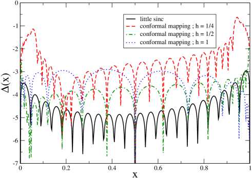
Figure 3: Error in the interpolation of $f(x)$ in eq.(40) using $21$ functions (color online).

Stenger originally introduced sinc methods for the numerical solution of differential equations Ste79 . Sinc-Galerkin and sinc collocation methods are particularly useful in dealing with these problems since they converge exponentially even in the presence of boundary singularities. It is not our purpose to generalize all the known mathematical results from the sinc functions to the LSF; however, we assume that both kind of functions share similar properties and simply compare our LSF results with those provided by the conformally mapped sinc functions.

We consider the example $4.1$ of Ref. Lybeck96 ; that is to say, the inhomogeneous differential equation 

$$-u^{\prime\prime}(x)+u^{\prime}(x)+u(x)=\left(\frac{4}{25}\right)^{2}\ \left(x^{4}-2x^{3}-29x^{2}+62x+38\right)$$ (41)

with the boundary conditions $u(-1)=u(4)=0$. The exact solution to this equation is

$$u_{exact}(x)=\left(\frac{4}{25}\right)^{2}\ (x+1)^{2}\ (x-4)^{2}\ .$$ (42)

We look for a numerical solution in terms of our LSF as

$$u(x)\approx u_{ls}(x)=\sum_{k=-N/2+1}^{N/2-1}u_{k}\ s_{k}(h,N,x-3/2)\ .$$ (43)

Fig. 4 shows global and local errors defined respectively as

$$\Xi_{G}(N) \equiv \log_{10}\left|\int_{-1}^{4}(u_{exact}(x)-u_{ls}(x))^{2}\ dx\right|$$ (44)

$$= \log_{10}\left|\int_{-1}^{4}u_{exact}^{2}(x)\ dx-h\sum_{k=-N/2+1}^{N/2-1}u^{2}_{k}\right|$$

$$\Xi_{L}(N) \equiv \log_{10}\left|(u_{exact}(3/2)-u_{ls}(3/2)\right|\ .$$ (45)

Notice that at large $N$ the errors appear to decay exponentially. Unlike Ref. Lybeck96 no domain decomposition was required to solve this problem.

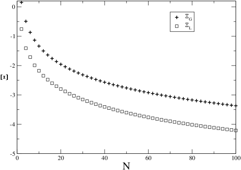
Figure 4: Global and local errors (44) and (45), respectively, for the solution of eq. (41) in terms of $N-1$ LSF.

Figure 5: Comparison between the exact solution $u_{true}(x)$ (solid line) and the approximations obtained using LSF with $N=4,6,10$ (color online).

IV The Schrödinger equation

As mentioned in the Introduction, sinc collocation methods have been used to obtain accurate numerical solutions to the Schrödinger equation. In this section we wish to extend the variational approach and the results of Ref. Amore06 to our LSF and generalize the method enclosing potentials with both bound and unbound states. To simplify this presentation we begin with potentials containing only bound states.

IV.1 Potentials containing only bound states

We consider the one dimensional Schrödinger equation

$$-\frac{\hbar^{2}}{2m}\frac{d^{2}\psi_{n}(x)}{dx^{2}}+V(x)\psi_{n}(x)=E_{n}\psi_{n}(x)$$ (46)

on an interval $(a,b)$, which can be either finite or infinite. The wave functions $\psi_{n}(x)$ obey the boundary conditions $\psi_{n}(a)=\psi_{n}(b)=0$ which grant that there will be only bound states.

If we express the wave functions in terms of our LSF, then equations (26), (28) and (32) allow one to derive the following matrix representation of the hamiltonian operator

$$H_{kl}=-\frac{\hbar^{2}}{2m}c_{kl}^{(2)}+\delta_{kl}V(kh)\ .$$ (47)

This equation is similar to eq.(8) of Ref. Amore06 , except for the form of the matrix $\mathbf{c}^{(2)}$. Once the spacing $h$ of the grid is fixed, then the $N\times N$ matrix $\mathbf{H}_{N}$ for a manifold of $N$ LSF can be diagonalized. In this way one obtains an approximation to the lower part of the spectrum, consisting of the first $N$ eigenvalues and wave functions of the Schrödinger equation (46).

Going back to eq. (47) we observe that the precision of the approximate results obtained by diagonalization of the hamiltonian matrix depends crucially on both the number of LSF as well as on the grid spacing. In fact, altough a small spacing can help to increase the resolution, if the number of the sinc functions is not large enough, the approximation will not be able to grasp the natural scale of the problem and the overall precision will be poor. On the other hand, a large spacing will certainly provide poor results, because the details of the problem will not be resolved. On these grounds it is easy to convince oneself that it is likely to exist an optimal spacing, for a given number of functions. Finding this optimal spacing will allow one to reach sufficiently accurate results with a relatively small number of grid points.

It was found earlier Amore06 that an optimal spacing can be obtained by straightforward application of the principle of minimal sensitivity (PMS) to the trace of the $N\times N$ hamiltonian matrix ${\cal T}_{N}(h)=Tr\left[\mathbf{H}_{N}\right]$. In fact, given that the trace of a hamiltonian is invariant under unitary transformations, and that in the limit $h\rightarrow 0$ it will therefore be independent of $h$, then the optimal spacing may be given by the solution of the equation 

$$\frac{d}{dh}{\cal T}_{N}(h)=0.$$ (48)

Therefore the optimal value of $h$ is found by numerically solving a single algebraic equation, a modest computational task; thus, the interval length $L$ appearing in LSF is treated as a variational parameter.

To test the performance of our method we apply it to the first example in Ref. Baye86 , i.e the harmonic oscillator with $\hbar=1$, $m=1/2$ and $\omega=2$. Using a cartesian mesh, Baye and Heenen reported errors smaller than $10^{-3}$ for the first three eigenvalues and $N=10$. On the other hand, our LSF approach with $N=10$ (which corresponds to $9$ sinc functions), and a grid spacing optimized according to eq. (48), yields errors of $-4.86\times 10^{-6}$, $1.2\times 10^{-4}$ and $-1.6\times 10^{-3}$ for the same cases.

The authors of Ref. Baye86 also observe that for $N=50$, the high eigenvalues become very sensitive to the value of $h$, and that the variation of the $30th$ eigenvalue with respect to $h$ presents a marked minimum around $h=0.35$. It is remarkable that the PMS condition for $N=50$ yields $L_{PMS}=8.93$, corresponding to $h_{PMS}=2L_{PMS}/N\approx 0.357$, which is extremely close to the value quoted by Baye and Heenen. It is worth noticing that while the optimal value of $h$ quoted by Baye and Heenen is the result of an empirical observation, the almost identical value of $h$ given by the PMS is just the numerical solution of the algebraic equation (48), which requires negligible computer time.

As a second example of application of the PMS to the LSF collocation method we consider the anharmonic potential

$$V(x)=x^{2}+x^{4}$$ (49)

and we assume that $\hbar=1$ and $m=1/2$ in the Schr̈odinger equation. This example was also studied by Baye and Heenen Baye86 who obtained the optimal values $h=0.55$ for $N=10$, and $h=0.2$ for $N=50$ using a cartesian mesh, which is somehow related to the LSF. Fig. 6 shows the error $|E_{0}^{exact}-E_{0}^{approx}|$ as a function of the parameter $L$ for three different values of $N$ (remember that the number of LSF in the expansion is $N-1$). The plus symbols in the plot correspond to the predictions of the PMS condition, which generally fall close to the minimum of the curve, while the square symbols correspond to the solutions of a sort of empirical PMS condition, obtained by minimizing the modified trace

$$\tilde{\cal T}_{N}(h)={\cal T}_{N}(h)-\frac{N-2}{2N}\sum_{k}V(x_{k})\ .$$ (50)

with respect to $L$. The better behavior of the modified PMS condition for just one state (as in Fig. 6) should not confuse the reader. It must be kept in mind that the PMS minimizes a sort of global error for all the states in the chosen manifold. In order to appreciate this point clearly, Fig. 7 shows the global error $\sigma=\sum_{n=0}^{N-1}|E_{n}^{(N)}-E_{n}^{(exact)}|$ as a function of $L$ for the potential $x^{4}/4$ and $N=20$. Notice that in this case the PMS condition yields the minimal error. The exact energies $E_{n}^{(exact)}$ were simply chosen to be those given by the method at higher order: $E_{n}^{(60)}$.

The accuracy of present calculations is greater than that obtained earlier for the same problem Baye86 , where the authors report errors of the order of $10^{-5}$ and $10^{-12}$ for $N=10$ and $N=50$, respectively. Fig. 6 shows that the curves with different values of $N$ overlap in the region of small $L$, which suggests that the approach may not be taking into account the large–$L$ region correctly.

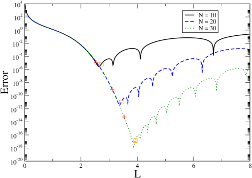
Figure 6: Error in the ground–state energy of the potential (49) using $N=10$, $20$ and $30$, as a function of the parameter $L$. The plus and square symbols correspond to the PMS and modified PMS conditions, respectively (color online).

Figure 7: Global error $\sigma\equiv\sum_{n=0}^{18}|E_{n}^{(20)}-E_{n}^{(60)}|$ for the potential $V(x)=x^{4}/4$ (color online).

IV.2 Potentials containing bound and unbound states

In what follows we try and show that the LSF are suitable for the treatment of potentials with bound and unbound states. The application of the PMS condition to potentials with both discrete and continuous spectra is not straightforward. The potentials treated in the preceding section increase with the coordinate and therefore the matrix representation of those potentials increase with $L$. Since the matrix representation of the kinetic energy decreases with $L$ then there is a minimum in the trace of the Hamiltonian matrix and the PMS gives a balance between the traces of the kinetic and potential energies. That minimum provides the natural length scale for the application of the method. If the potential energy tends to a finite constant value as the coordinate increases, then there may not be a minimum and the PMS will not yield the length scale for the application of present approach.

In order to overcome that problem we substitute a potential $\tilde{V}(x)$ into the Schrödinger equation that behaves exactly as the original potential $V(x)$ in the relevant coordinate region and increases to infinity at large distances. The error introduced by such potential substitute will be negligible if the difference between the original and substitute potentials is appreciable only where the wavefunctions are expected to be vanishing small. This substitution removes the continuous spectrum but should not affect the discrete one too much. The advantage is that we are thus able to apply the PMS condition exactly as in the preceding subsection. The potential substitute is introduced with the sole purpose of obtaining the length scale and we diagonalize the correct hamiltonian matrix.

We will illustrate our procedure on the Morse potential already treated earlier by means of the Lagrange mesh method BGV02 :

$$V(r)=D\ \left[e^{-2a(r-r_{e})}-2e^{-a(r-r_{e})}\right]\ ,$$ (51)

where $D=0.10262$, $r_{e}=2$, $a=0.72$, $2m=1836$ and $\hbar=1$. In the case of states with nonzero angular momentum we should add the centrifugal potential $\frac{\hbar^{2}l(l+1)}{2mr^{2}}$, $l=0,1,2,\dots$.

The potential substitute $\tilde{V}(r)$ is arbitrary; we can, for example, choose it to be the Taylor expansion of $V(r)$ around a given point, and truncate it at a sufficiently large order to be accurate enough at small $r$, and at the same time to satisfy $\lim_{r\rightarrow\infty}\tilde{V}(r)=+\infty$. For example, in present particular case we can choose:

$$\tilde{V}(r)=\sum_{n=0}^{20}\frac{1}{n!}\ \left.\frac{d^{n}V}{dr^{n}}\right|_{r=10}(r-10)^{n}\ .$$ (52)

Another difficulty to take into consideration is that our LSF are defined in $(-L,L)$ whereas the radial coordinate is defined in $(0,+\infty)$. The obvious solution to this apparent problem would be using the form of Ref. Baye95 , where the left boundary of the interval is $0$; on the other hand, such choice would be equivalent to a shift by a proper amount of the potential, thus bringing the boundary condition on the left point to coincide with the left point of the LSF. Despite its simplicity, this procedure is not optimal and generally does not provide the best results. We have found out that a more convenient strategy consists of keeping our LSF unchanged and shifting the coordinate by given amount as $V(r)\rightarrow V(r+\overline{r})$, where $\overline{r}$ is typically close to the minimum of the potential (the same shift should be applied to the centrifugal energy when necessary). The PMS applied to the shifted hamiltonian will thus provide the optimal scale for the application of the LSF collocation method.

One advantage of that procedure is that it maximizes the sampling of the classically allowed region, where the bound state wave functions exhibit marked nonzero contributions. Of course, in order to take into account the boundary condition at $r=0$, the PMS length scale has to be smaller than $\overline{r}$.

Table 1: Errors $\epsilon_{n}\equiv E_{n}^{approx}-E_{n}^{exact}$ for some states of the Morse potential. Powers of ten are indicated between square brackets.

$l$	$n$	$N$	Ref.BGV02	PMS	$h_{PMS}$
$0$	$0$	$20$	$3.8[-7]$	$-3.3[-10]$	$0.223$
		$40$	$<1[-14]$	$1.8[-20]$	$0.134$
	$5$	$20$	$4.0[-3]$	$2.1[-6]$	$0.223$
		$40$	$1.1[-9]$	$2.5[-14]$	$0.134$
$1$	$0$	$20$	$4.1[-7]$	$-3.6[-10]$	$0.223$
		$40$	$<1[-14]$	$-1.6[-20]$	$0.134$
	$5$	$20$	$4.4[-3]$	$1.5[-6]$	$0.223$
		$40$	$1.1[-9]$	$2.9[-14]$	$0.134$
$2$	$0$	$20$	$4.5[-7]$	$-4.1[-10]$	$0.223$
		$40$	$<1[-14]$	$1.2[-20]$	$0.134$
	$5$	$20$	$4.7[-3]$	$2.0[-7]$	$0.223$
		$40$	$1.1[-9]$	$3.9[-14]$	$0.134$

Figure 8: Error $\eta_{N}(x)=|\psi^{(N)}(x)-\psi^{(80)}(x)|$ as a function of $x$ for the ground state of the Morse potential (color online).

Table 1 shows the errors $\epsilon_{n}\equiv E_{n}^{approx}-E_{n}^{exact}$ for the s, p, and d states of the Morse potential with $n=0$ and $n=5$. It compares present results with those of Baye et al BGV02 . The last column of Table 1 displays the PMS optimal values of the grid spacing.

Fig. 8 shows the local error $\eta_{N}(x)=|\psi^{(N)}(x)-\psi^{(80)}(x)|$ for the ground state of the Morse potential and approximations $N=20$ and $N=40$, where we have chosen $\overline{r}=3$. We assume that the approximation of order $N=80$ is sufficiently close to the exact wavefunction. Our results are more accurate than those of Baye et al BGV02 who essentially considered the average of $\eta(x)$ over a chosen region. The sharp drop of the error beyond a certain value of $r$, clearly noticeable in Fig. 8, is due to the fact that our LSF reproduce the wave function only in a finite region outside which $\eta(x)$ is merely the value of $\psi^{(80)}(x)$. It is worth noticing that $\eta_{N}(x)$ is almost uniform in the region covered by the LSF.

We have also applied our method to the one–dimensional Morse potential considered by Wei Wei00 :

$$V(x)=D\left[e^{-2\alpha x}-2e^{-\alpha x}+1\right],$$ (53)

where $-\infty<x<\infty$, $D=0.0224$, $\alpha=0.9374$, $m=119406$ and $\hbar=1$. This problem can be solved exactly and the energies are given by Marcelo

$$E_{n}=\hbar\omega\left[n+\frac{1}{2}-\frac{\hbar\omega}{4D}\left(n+\frac{1}{2}\right)^{2}\right]$$ (54)

where $\omega=\sqrt{2D/m}\ \alpha$. As before we can improve our results by conveniently shifting the potential on the $x$-axis from $V(x)$ to $V(x+\overline{x})$. When $N=20$ and assuming $\overline{x}=0$ we have found that the first–excited–state eigenvalue is reproduced with an accuracy of about $8\times 10^{-14}$, which is even better than the accuracy obtained by Wei with $N=64$ . When $N=40$ the error of our method is just $8.1\times 10^{-21}$ for the ground state.

V Conclusions

In this paper we have introduced a new class of sinc-like functions, which we name “little sinc functions” (LSF), which share some properties of the usual sinc functions, but are defined on finite intervals. We have shown that the LSF collocation method provides accurate approximations for a wide class of problems when it is supplemented by the Principle of Minimal Sensitivity (PMS) that provides an optimal grid spacing. In particular, we have applied the LSF to the solution of the Schrödinger equation with only bound states and with mixed discrete and continuous spectra. We have chosen benchmark models treated earlier by other authors and in all the cases we obtained more accurate results. It seems that the LSF collocation method is an interesting alternative algorithm for solving many mathematical and physical problems.

- (1) D. Baye, Constant-step Lagrange meshes for central potentials, Journal of Physics B 28, 4399-4412 (1995)
- (2) D. Baye and P.H. Heenen, Generalised meshes for quantum mechanical problems, Journal of Physics A 2041-2059 (1986)
- (3) D. Baye, M.Hesse and M.Vincke, The unexplained accuracy of the Lagrange-mesh method, Phys.Rev.E 65, 026701 (2002)
- (4) V.G. Koures and F. E. Harris, International Journal of Quantum Chemistry 30,1311 (1996)
- (5) F. Stenger, Numerical methods based on sinc and analytic functions, Springer-Verlag,New York, 1993
- (6) F. Stenger, A sinc-Galerkin method of solution of boundary value problems, Math. Comp. 33 , 85-109 (1979)
- (7) A.C. Morlet, Siam Journal on Numerical Analysis 32 (1995) 1475-1503
- (8) N.J. Lybeck and K.L. Bowers, Sinc methods for domain decomposition, Applied Mathematics and Computation 75 (1996) 13-41
- (9) S. Narashiman, J. Majdalani and F. Stenger, A first step in applying the sinc collocation method to the nonlinear Navier-Stokes equations, Numerical Heat transfer 41 (2002) 447-462
- (10) R. Easther, G. Guralnik and S. Hahn, Phys. Rev. D 61, 125001 (2000)
- (11) R. Revelli and L. Ridolfi, Computers and mathematics with applications 46, 1443-1453 (2003)
- (12) P. Amore, A variational sinc collocation method for strong coupling problems, Journal of Physics A 39, L349-L355 (2006)
- (13) P. M. Stevenson, Phys. Rev. D 23, 2916 (1981).
- (14) P. Amore, A. Aranda, H.F. Jones and F.M. Fernández, A new approximation method for time independent problems in quantum mechanics, Physics Letters A 340, 201-208 (2005)
- (15) G.W. Wei, Solving quantum eigenvalue problems by discrete singular convolution, Journal of Physics B 33, 343-352 (2000)
- (16) F.M. Fernández, Introduction to perturbation theory in quantum mechanics, CRC press (2001)