Entanglement and Symmetry: A Case Study in
Superselection Rules, Reference Frames, and Beyond

Abstract

In recent years it has become apparent that constraints on possible quantum operations, such as those constraints imposed by superselection rules (SSRs), have a profound effect on quantum information theoretic concepts like bipartite entanglement. This paper concentrates on a particular example: the constraint that applies when the parties (Alice and Bob) cannot distinguish among certain quantum objects they have. This arises naturally in the context of ensemble quantum information processing such as in liquid NMR. We discuss how a SSR for the symmetric group can be applied, and show how the extractable entanglement can be calculated analytically in certain cases, with a maximum bipartite entanglement in an ensemble of $N$ Bell-state pairs scaling as $\log(N)$ as $N\to\infty$. We discuss the apparent disparity with the asymptotic ($N\to\infty)$ recovery of unconstrained entanglement for other sorts of superselection rules, and show that the disparity disappears when the correct notion of applying the symmetric group SSR to multiple copies is used. Next we discuss reference frames in the context of this SSR, showing the relation to the work of von Korff and Kempe [Phys. Rev. Lett. 93, 260502 (2004)]. The action of a reference frame can be regarded as the analog of activation in mixed-state entanglement. We also discuss the analog of distillation: there exist states such that one copy can act as an imperfect reference frame for another copy. Finally we present an example of a stronger operational constraint, that operations must be non-collective as well as symmetric. Even under this stronger constraint we nevertheless show that Bell-nonlocality (and hence entanglement) can be demonstrated for an ensemble of $N$ Bell-state pairs no matter how large $N$ is. This last work is a generalization of that of Mermin [Phys. Rev. D 22, 356 (1980)].

I Introduction

The entanglement of disjoint (typically spatially separate) quantum systems is at the heart of quantum information processing  NieChu00 . For bipartite pure states under LOCC (local operations and classical communication) the quantification and transformation of entanglement is now well understood. However, it is also now well understood that the non-ideal situation of mixed states, which pertains in practice, is far more complicated (or richer, to put a different spin on it) Hor01 . In recent years it has also become apparent that a situation, in which only certain operations can be performed, also leads to an interesting theory of entanglement, even if the states are pure. One approach, leading to a generalized notion of entanglement, dismisses altogether with the bipartite setting Barnum03 ; Barnum04 . A less radical, and more obviously applicable, idea is to restrict the local operations to those that are invariant under a superselection rule (SSR) Ver03 ; WisVac03 ; BarWis03 ; KMP04 ; SchVerCir04 ; BarDohSpeWis06 ; VacAnsWisJac06 . At the same time, the nature of quantum reference frames in the bipartite setting has also been hotly debated (see for example Refs. RudSan01 ; EnkFuc02a ; SanBarRudKni03 ; Wis04 ).

Much of the work in this area Ver03 ; WisVac03 ; SchVerCir04 ; BarDohSpeWis06 ; RudSan01 ; EnkFuc02a ; SanBarRudKni03 ; Wis04 has concentrated upon the case of a U(1)-SSR. This is the SSR that can be motivated by considering the conservation of a locally additive scalar quantity with a discrete spectrum Wis04 . It can also be applied to quantum optics experiments which lack an optical phase reference (that is, which lack a shared clock of sufficient precision) SanBarRudKni03 . Many simplifications arise from this SSR because U(1) is Abelian (there is only one generator, corresponding to the local operator of the conserved quantity). Non-Abelian Lie-group SSRs (with non-commuting generators) have also been considered KMP04 but relatively little attention has been paid to SSRs arising from discrete groups. An example with obvious application to ensemble quantum information processing is the symmetric group $S_{N}$ (the group of permutations of $N$ objects) BarWis03 .

This paper explores issues in entanglement under operations constrained by symmetry. We use the $S_{N}$-SSR formalism of Ref. BarWis03 , but also go beyond that work. This work is important for a number of reasons. First, as noted above, the symmetric group has been relatively neglected in studies of entanglement constrained by a SSR. For the U(1)-SSR concepts like bound entanglement (of two distinct types), activation, and distillation have been shown to apply, in analogy to these concepts in mixed-state entanglement. Although not immediately obvious, we construct specific examples to show how these concepts apply to the $S_{N}$-SSR. Second, we clarify the notion of a reference frame for the $S_{N}$ group, linking in with the work of von Korff and Kempe vKK04 . Finally, we give an example where it is not obvious that the symmetry constraints on the system can be formulated as a SSR. Nevertheless we show that, even under such constraints, it is possible to exhibit Bell-nonlocality Bel64 for an ensemble of identically prepared singlets.

II Entanglement and SSRs

II.1 Concepts of Entanglement

The term entanglement was coined by Schrödinger Sch35 as the property that bipartite pure states have when they are not product states. Schrödinger showed that for such an entangled state, one party (say Bob) could, via a measurement on his system, collapse Alice’s system with some probability to any state vector (except those in the null space of Alice’s reduced state matrix). Schrödinger thought this nonlocality was unreasonable enough to be called a “paradox” Sch36 . A generation later, Bell Bel64 discovered that such states had an even stronger form of nonlocality: for certain measurement schemes, the correlations between the results of Alice and Bob cannot be explained by any locally causal theory. This property, which we will call Bell-nonlocality, we regard as the strongest operational notion of entanglement.

II.1.1 Separability and Local Preparability

When correlations in mixed states were first studied in earnest Wer89 , it became clear that the question as to whether a state was entangled was no longer straightforward. In particular, Werner showed that there were nonseparable states such that the measurement correlations of Alice and Bob could nevertheless be explained by a local theory involving hidden variables. Nonseparable states are states that cannot be written in the form

$$\rho = \sum_{k}\wp_{k}|\psi_{k}\rangle\langle\psi_{k}|\otimes|\phi_{k}\rangle\langle\phi_{k}|$$ (1)

$$\equiv \biguplus_{k}\sqrt{\wp_{k}}\left({|{\psi_{k}}\rangle\otimes|{\phi_{k}}\rangle}\right)$$

$$\equiv \uplus\sqrt{\wp_{1}}\left({|{\psi_{1}}\rangle\otimes|{\phi_{1}}\rangle}\right)\uplus\sqrt{\wp_{2}}\left({|{\psi_{2}}\rangle\otimes|{\phi_{2}}\rangle}\right)\uplus\cdots$$

Here, following Ref. VacAnsWisJac06 , we have defined a notation that we will use throughout this paper, that for an arbitrary ray $|{r}\rangle$, we have $\uplus|{r}\rangle\equiv+|{r}\rangle\langle{r}|$. Werner called nonseparable states “EPR correlated states”. They are sometimes identified with “entangled” states but we will call them non-locally-preparable states. This name captures the physical significance of such states: they cannot be prepared by LOCC from a product state.

II.1.2 $n$-Distillability and Bound Entanglement

Since Werner, the richness of the entanglement of mixed states has been further developed, involving concepts such as bound entanglement, distillation, $n$-distillability, and activation Hor01 . Here, following Ref. BarDohSpeWis06 , we concentrate upon those properties of mixed state entanglement for which there are obvious analogs in pure state entanglement constrained by SSRs. First, as noted above, it is useful to define the class of locally preparable states, which are those states that are preparable from a product state using LOCC. Another useful class is the class of states that are distillable Ben96 . States in the distillable class are such that $n$ copies can be converted into $nr$ pure maximally entangled states via LOCC for some $r>0$ in the limit $n\to\infty$. A pure state is either locally preparable or distillable, depending on whether it is a product state or not. On the other hand, there are mixed states that are neither locally preparable nor distillable. These are the so-called bound entangled states Hor98 .

For mixed states, deciding whether a state is locally preparable is known to be an NP-hard problem computationally Gur02 , but algorithms to do so exist DohParSpe02 . It is not known if it is even possible to determine whether a state is distillable. For this reason, a related, but simpler to characterize, class has been defined: the states that are 1-distillable Div00 ; Dur00 . A state $\rho$ is 1-distillable if by LOCC Alice and Bob can, with some probability, create from it a non-separable two-qubit state. (Note that for two qubits, there are no bound entangled states Hor97 .) By extension, a state $\rho$ is $n$-distillable if $\rho^{\otimes n}$ is 1-distillable. (If a state is $n$-distillable for some $n$ then it is distillable.) Thus, the set of distillable states includes the 1-distillable states, and in fact it has recently been shown that the $n$-distillable states are a subset of the distillable states $\forall\ n$ Wat04 . Since the 1-distillable states are a subset of distillable states, there are clearly mixed states that are neither locally preparable nor 1-distillable. We shall refer to these states as being 1-bound.

Note that although a nonseparable two-qubit state is always distillable, this does not mean that undistilled copies can be used to demonstrate Bell-nonlocality, as Werner showed Wer89 . However, in our work pertaining to SSRs, when we demonstrate that a state is 1-distillable, we do this by showing that it is possible for Alice and Bob by LOCC to create with some probability a pure entangled state, as this is strictly stronger than the requirements for being 1-distillable. Thus, for these purposes, a state that is 1-distillable allows Alice and Bob to demonstrate Bell-nonlocality, which, as noted above, we regard as the strongest notion of entanglement.

II.1.3 Closing the gap: PPT-Channels

Returning to the 1-bound states in general, this class can be divided into two by considering what would happen if we were to give Alice and Bob a PPT-channel. That is, a channel that can distribute only bipartite states for which the partial transpose is positive. This allows Alice and Bob to perform PPT-operations as well as LOCC. A PPT operation is one that preserves the positivity of the partial (with respect to Alice or Bob) transpose of states Rai01 . With this addition, Alice and Bob can locally prepare all states with a positive partial transpose, which includes some states which are 1-bound Hor98 . We will call these the bound states that become locally preparable.Conversely, the rest of the 1-bound states, those that are not PPT, become 1-distillable under LOCC plus all PPT operations Egg01 . Hence we call this class (which is also non-empty Wat04 ) become 1-distillable.

II.1.4 Activation

Physically, a PPT-channel is equivalent to supplying Alice and Bob with an infinite number of copies of every state in the become locally preparable class.Access to these states automatically makes them locally preparable. However, it is not necessary to use all of the states to make 1-distillable a state in become 1-distillable. Rather, for every $\rho$ in become 1-distillable there exists a state $\sigma$ in become locally preparable such that $\rho\otimes\sigma$ is 1-distillable. This is known as activation Hor99 . Note the distinction from distillation, in which for some $\rho$ which is in become 1-distillable, there exists an $n$ such that $\rho^{\otimes n}$ is 1-distillableWat04 . Note that it is trivially the case that any state $\rho$ which can become locally preparable does so given a suitable state $\sigma$ which can become locally preparable: one simply chooses $\sigma=\rho$.

II.1.5 Measures of Entanglement

Finally for this section, we define some measures of entanglement. The entanglement of formation, $E_{F}$, of a mixed state $\rho$ is the minimum ratio, in the asymptotic limit, of the number of singlets used to the number of copies of $\rho$ created thereby, using LOCC HillWoot97 . Similarly, the distillable entanglement, $E_{D}$, is the asymptotic yield of arbitrarily pure singlets that can be prepared by LOCC from copies of $\rho$ BennetDiVSmolWoot96 . By definition, both of these measures are partially additive. That is, $n$ copies of a state $\rho$ contains $n$ times the entanglement of a single copy; $E(\rho^{\otimes n})=nE(\rho)$. Also by definition Hor99 , and the fact that LOCC cannot increase entanglement, $E_{F}$ is an upper bound on $E_{D}$. In general it is a strict upper bound, which is obvious from the existence of bound entangled states where $E_{F}\neq 0$ when $E_{D}=0$. However for pure states $E_{F}=E_{D}$. Since we will be concerned with states that can be made pure by LOCC, there is no need to distinguish between $E_{F}$ and $E_{D}$. For a bipartite pure state $|{\Psi}\rangle$ the entanglement (measured in e-bits BennetDiVSmolWoot96 ) is defined as the von Neumann entropy of either subsystem’s reduced density matrix,

$$E(|{\Psi}\rangle)=-{\rm Tr}\left[{{\rho_{A}\log_{2}\rho_{A}}}\right]=-{\rm Tr}\left[{{\rho_{B}\log_{2}\rho_{B}}}\right],$$ (2)

where the reduced density matrices for Alice and Bob are defined as $\rho_{A}={\rm Tr_{B}}[|{\Psi}\rangle\langle{\Psi}|]$ and $\rho_{B}={\rm Tr_{A}}[|{\Psi}\rangle\langle{\Psi}|]$ respectively. ${\rm Tr_{A,B}}$ signifies the partial trace operation with respect to Alice or Bob.

II.2 Superselection Rules

II.2.1 SSRs as an Operational Restriction

Originally Wic52 , SSRs were regarded as restrictions on the states that a system can be in. This could be restated operationally, as a restriction on the means of preparing a system. Since any operation could be part of a system-preparation procedure, it is only sensible to say that a SSR is a restriction on the operations that can be performed on a system. For an SSR for charge (the first such SSR ever proposed) Wic52 , this restriction would amount to saying that it is not possible to create superpositions of different charge eigenstates. Alternatively, all operations on the system must commute with charge-preserving operations such as measurement of charge. Charge-preserving operations can be built up from transformations in the Lie group U(1) generated by the charge operator. This formulation allows the concept of SSRs to be generalized to arbitrary compact Lie groups, or finite groups BarWis03 ; KMP04 , as we now explain.

The SSR for a group $G$ of physical transformations can be defined operationally as follows. Consider for the moment a single party, Alice, who possesses a quantum system, described by a Hilbert space $\mathbb{H}_{A}$. Let the physical transformation corresponding to an element $g$ of $G$ be denoted $\hat{T}_{A}(g)$. Then the $G$-SSR is the rule that all operations must be $G$-invariant. That is, if ${\cal O}$ is the completely positive map $\rho\to{\cal O}{\rho}$ representing the operation, then

$$\forall\rho\textrm{ and }\forall g\in G\,,\;{\cal O}[\hat{T}_{A}(g)\rho\hat{T}^{\dagger}_{A}(g)]=\hat{T}_{A}(g)[{\cal O}\rho]\hat{T}^{\dagger}_{A}(g).$$ (3)

Note that “operations” includes unitaries, where ${\cal O}\rho=\hat{U}\rho\hat{U}^{\dagger}$, and also measurements, where for example ${\cal O}_{r}\rho=\hat{M}_{r}\rho\hat{M}_{r}^{\dagger}$ and $\sum_{r}\hat{M}_{r}^{\dagger}\hat{M}_{r}=\hat{1}$.

According to this definition, we would say that a SSR for charge $\hat{Q}_{A}$, for example, would be a SSR for the group U(1) generated by $\hat{Q}_{A}$. Such a SSR can be motivated from consideration of a conservation law for global charge $\hat{Q}_{A}$. Note however that we do not assume that the operational restriction described by a general SSR must be derivable from a conservation law. For the purposes of this paper, it is more fruitful to regard a $G$-SSR as being due to the lack (by Alice) of an appropriate reference frame AhaSus67 ; BarRudSpe05 ; BarDohSpeWis06 . This idea will be explored later in the particular context of the $S_{N}$-SSR.

II.2.2 SSRs and Mixing

All quantum information processing ultimately ends in measurement. If a $G$-SSR is in force over the entire process, then no outcomes will be changed if the state matrix for the quantum system $\rho$ is replaced by the state matrix $\hat{T}_{A}(g)\rho\hat{T}^{\dagger}_{A}(g)$ for any $g\in G$. That is, under the $G$-SSR the state of the quantum system is represented by an equivalence class of state matrices. The most mixed state matrix to which $\rho$ is physically equivalent is

$$\mathcal{G}_{A}\rho\equiv|G|^{-1}\sum_{g\in G}\hat{T}_{A}(g)\rho\hat{T}^{\dagger}_{A}(g)$$ (4)

for finite groups, where $|G|$ is the group order, and

$$\mathcal{G}_{A}\rho\equiv\int_{{}_{G}}\text{d}\mu(g)\,\hat{T}_{A}(g)\rho\hat{T}^{\dagger}_{A}(g)$$ (5)

for compact Lie groups, where $\text{d}\mu(g)$ is the Haar measure. We call this the $G$-invariant state, as

$$\forall g\in G,\;\hat{T}_{A}(g)[\mathcal{G}_{A}\rho]\hat{T}^{\dagger}_{A}(g)=\mathcal{G}_{A}\rho.$$ (6)

For traditional SSRs, i.e. groups with a single generator $\hat{Q}_{A}=\sum_{q}q\,\hat{\Pi}_{q}$, the $G$-invariant state is simply the block-diagonal state ${\cal G}_{A}\rho=\sum_{q}\,\hat{\Pi}_{q}\,\rho\,\hat{\Pi}_{q}.$

This maximum-entropy member of the equivalence class is the one containing no irrelevant information, and hence it is the natural representation of the state of the system as a state matrix. This state can also be given an operational interpretation VacAnsWisJac06 . Given the $D$-dimensional quantum system with state $\rho$ and a heat bath at temperature $T$, work can be extracted by allowing the system to come to thermal equilibrium. The maximum amount of extractable work is $k_{\rm B}T[\log D-S(\rho)]$, where $S$ is the von Neumann entropy OppHor02 . Under the constraint of a $G$-SSR, the amount of extractable work is reduced by (the positive quantity) $k_{\rm B}T\Delta_{G}(\rho)$, where $\Delta_{G}(\rho)=S({\cal G}_{A}\rho)-S(\rho)$ is precisely the amount of “irrelevant information” in $\rho$.

It is very important to note that if Alice has two systems with states $\rho_{1}$ and $\rho_{2}$, such that ${\cal G}_{A}(\rho_{1}\otimes\rho_{2})$ equals

$$|G|^{-1}\sum_{g\in G}[\hat{T}_{1}(g)\otimes\hat{T}_{2}(g)]\rho[\hat{T}_{1}^{\dagger}(g)\otimes\hat{T}_{2}^{\dagger}(g)],$$ (7)

then this state is not the same as ${\cal G}_{A}\rho_{1}\otimes{\cal G}_{A}\rho_{2}$, which equals

$$|G|^{-2}\sum_{g,g^{\prime}\in G}[\hat{T}_{1}(g)\otimes\hat{T}_{2}(g^{\prime})]\rho[\hat{T}_{1}^{\dagger}(g)\otimes\hat{T}_{2}^{\dagger}(g^{\prime})].$$ (8)

That is why in the above we have referred to the quantum system, not a quantum system. If we are considering the whole quantum system (or at least all parts to which the SSR applies), then the state $\rho$ of the system can be replaced by ${\cal G}_{A}\rho$. But if there are other quantum systems that may enter into the quantum information processing at a later time, then it is not true in general that ${\cal G}_{A}\rho$ contains all of the relevant information about that system.

II.2.3 Bipartite SSRs

In this paper we are concerned with the impact of SSRs on entanglement, rather than extractable work (although the latter is, in the bipartite setting, also related to entanglement VacAnsWisJac06 ). In this context we have to define the concept of local SSRs. That is, the local operations of Alice and Bob (say) must respect local SSRs, rather than a global SSR. This is obviously applicable in the case when a SSR is motivated by a conservation law for a locally additive quantity. It is also applicable more generally if Alice and Bob each lack a reference frame. It turns out that for the purpose of non-local quantum information processing, what is important is that Alice and Bob have a shared reference frame. Furthermore, such a reference frame need only be correlated between the two parties. This point will be clarified by later examples.

For the concept of a local SSR or local reference frame to make sense, the physical transformation on the joint Hilbert space $\mathbb{H}_{A}\otimes\mathbb{H}_{B}$ corresponding to an element $g$ of the group $G$ must have the following form:

$$\hat{T}(g)=\hat{T}_{A}(g)\otimes\hat{T}_{B}(g).$$ (9)

Now if Alice and Bob lack reference frames, then the effective state for the bipartite system is the locally $G$-invariant state BarWis03

$$({\cal G}_{A}\otimes{\cal G}_{B})\rho,$$ (10)

where ${\cal G}_{A}$ is defined as above, and ${\cal G}_{B}$ similarly, and these act locally according to the tensor-product structure of the joint system. Note that this state is in general very different from the globally $G$-invariant state

$${\cal G}\rho=\sum|G|^{-1}\sum_{g\in G}[\hat{T}_{A}(g)\otimes\hat{T}_{B}(g)]\rho[\hat{T}_{A}^{\dagger}(g)\otimes\hat{T}_{B}^{\dagger}(g)].$$ (11)

Just as in the case of a single party, it is important to remember that $\rho$ can be replaced by $({\cal G}_{A}\otimes{\cal G}_{B})\rho$ only if it is the state of the entire quantum system shared by Alice and Bob (or at least all parts to which the SSR applies).

II.2.4 SSRs and Hilbert Space (Technicalities)

To determine the effect of SSRs on entanglement it is necessary to understand how a SSR induces a structure on Hilbert space. A local $G$-SSR for Alice splits $\mathbb{H}^{A}$ into “charge sectors” labeled by $y$:

$$\mathbb{H}^{A}=\bigoplus_{y}\mathbb{H}^{A}_{y},$$ (12)

where each $\mathbb{H}^{A}_{y}$ carries inequivalent representations $\hat{T}^{A}_{y}$ of $G$. The sectors are then further decomposed into tensor products:

$$\mathbb{H}^{A}_{y}=\mathbb{M}^{A}_{y}\otimes\mathbb{Q}^{A}_{y}.$$ (13)

This is technically known as dividing the system into subsystems. The subsystem $\mathbb{M}^{A}_{y}$ carries an irreducible representation (irrep) $\hat{t}^{A}_{y}(g)$ and the subsystem $\mathbb{Q}^{A}_{y}$ carries a trivial representation of $G$. That is to say,

$$\hat{T}^{A}_{y}(g)=\hat{t}^{A}_{y}(g)\otimes\hat{I}^{A}_{y}.$$ (14)

For an Abelian SSR such as charge, the subsystems $\mathbb{M}^{A}_{y}$ are one-dimensional, and so the additional tensor product structure within the irreps is not required. However, for a non-Abelian SSR such as we will consider later, they are nontrivial.

The subsystems $\mathbb{Q}^{A}_{y}$ are clearly $G$-invariant. They have been called noiseless subsystems, or decoherence-free subsystems, relative to the decoherence map $\mathcal{G}_{A}$ Kni00 . By contrast, the subsystems $\mathbb{M}^{A}_{y}$ become completely mixed under the action of $\mathcal{G}_{A}$, because $\hat{t}^{A}_{y}(g)$ is irreducible. Thus the action of $\mathcal{G}_{A}$ on an arbitrary state matrix $\rho$ is, in terms of this decomposition,

$$\mathcal{G}_{A}\rho=\sum_{y}\mathcal{D}^{A}_{y}\otimes\mathcal{I}^{A}_{y}(\hat{\Pi}^{A}_{y}\rho\hat{\Pi}^{A}_{y}).$$ (15)

Here $\hat{\Pi}^{A}_{y}$ is the projection onto the charge sector $y$, $\mathcal{D}^{A}_{y}$ is the trace-preserving map that takes every operator for the subsystem $\mathbb{M}^{A}_{y}$ to a maximally mixed operator (i.e. proportional to the identity operator on that space), and $\mathcal{I}^{A}_{y}$ is the identity map over operators for the subsystem $\mathbb{Q}^{A}_{y}$. The effect of the local superselection rule, then, is to remove the coherence between different local charge sectors (as in the Abelian case) and to make the subsystems $\mathbb{M}^{A}_{y}$ completely mixed. The same structure arises for $\mathbb{H}^{B}$ and provides an analogous decomposition of $\mathcal{G}_{B}$. For further details, see BarWis03 ; KMP04 .

II.3 Concepts of Entanglement Constrained by SSRs

In this section we summarize the results of Ref. BarDohSpeWis06 , showing the analogies between mixed-state entanglement and pure-state entanglement constrained by a SSR. The various concepts of entanglement explored in Sec. II.1 arise from considering two parties able to perform LOCC. Adding the constraint of a local $G$-SSR (that is, that the local operations must be $G$-invariant) we say that the two parties can perform $G$-LOCC.

II.3.1 Local Preparability

The class of pure bipartite states that are locally preparable under $G$-LOCC will call ${G\text{-SSR}}$ locally preparable. Just as preparable under LOCC means preparable from states that are local (separable), so preparable under $G$-LOCC means preparable from states that respect the $G$-SSR (i.e. that are locally $G$-invariant). It is trivial to see that a pure bipartite state $|{\psi}\rangle$ is ${G\text{-SSR}}$ locally preparable iff (i) the state is a product state, and (ii) it is locally $G$-invariant. Note that not all pure product states are ${G\text{-SSR}}$ locally preparable; it is a smaller class than the locally preparable states.

II.3.2 $n$-Distillability and Bound Entanglement

The class of pure states that are 1-distillable under $G$-LOCC, which we call ${G\text{-SSR}}$ 1-distillable, is defined as those states $|{\psi}\rangle$ for which the following is true: The two parties can, by local measurements, project $|{\psi}\rangle$ onto a $2{\times}2$-dimensional subspace with nonzero probability, such that the projected state is (i) locally $G$-invariant and (ii) non-separable. The significance of the first condition is that the SSR is now irrelevant, so that the usual condition (nonseparability) is all that is required for 1-distillability. It is not difficult to see BarWis03 that $|\psi\rangle$ is ${G\text{-SSR}}$ 1-distillable iff $\mathcal{G}_{A}\otimes\mathcal{G}_{B}[|\psi\rangle\langle\psi|]$ is 1-distillable under LOCC.

Both the class of ${G\text{-SSR}}$ locally preparable and ${G\text{-SSR}}$ 1-distillable states are non-empty in general (i.e. for a general SSR). Moreover, as with mixed-state entanglement, there is a proper gap between these two classes. The class of states in the gap contains both product and non-product pure states, and is analogous to the class of 1-bound states in mixed-state entanglement.

The concepts of $n$-distillability with the SSR constraint (and the corresponding classes of pure states, ${G\text{-SSR}}\ n$-distillable) can be defined analogously to the case of unconstrained entanglement. It is not difficult to illustrate the phenomenon of distillation; that is, to find examples of states that are ${G\text{-SSR}}$ distillable but not ${G\text{-SSR}}$ 1-distillable KMP04 . Here ${G\text{-SSR}}\ {\rm distillable}={G\text{-SSR}}\ \infty$-distillable is the class of distillable pure states under this constraint.

II.3.3 Closing the gap

Just as in mixed-state entanglement adding a PPT channel removes the 1-bound class, so it is possible to augment $G$-LOCC in such a way that any pure state in the gap between ${G\text{-SSR}}$ locally preparable and ${G\text{-SSR}}$ 1-distillable becomes either locally preparable or 1-distillable. In this case the augmentation is very simple: one simply lifts the restriction of the local SSR by providing Alice and Bob with a shared reference frame.With this additional resource, Alice and Bob can now implement any operation in LOCC.

Augmenting $G$-LOCC to LOCC divides the proper gap of pure states between ${G\text{-SSR}}$ locally preparable and ${G\text{-SSR}}$ 1-distillable into two classes, both of which are non-empty. All product states that are not locally $G$-invariant (i.e., product states not in ${G\text{-SSR}}$ locally preparable) become locally preparable with $G$-LOCC plus the shared reference frame for $G$. We call this class ${G\text{-SSR}}$ become locally preparable. This result follows directly from the fact that all pure product states are locally preparable with unrestricted LOCC. Similarly all non-product pure states which are not in ${G\text{-SSR}}$ 1-distillable become 1-distillable under $G$-LOCC plus the shared reference frame for $G$. We thus call this class ${G\text{-SSR}}$ become 1-distillable. This result follows directly from the fact that all pure non-product states are 1-distillable with unrestricted LOCC.

II.3.4 Activation

Again, just as in the mixed-state case, it is not necessary to completely lift the SSR constraint in order to make any particular state $|{\psi}\rangle$ either ${G\text{-SSR}}$ locally preparable or ${G\text{-SSR}}$ 1-distillable. Rather, all that is needed is some other pure state $|{\phi}\rangle$ which is ${G\text{-SSR}}$ become locally preparable. Again, this is trivial if $|{\psi}\rangle$ is ${G\text{-SSR}}$ become locally preparable; one simply chooses $|{\phi}\rangle=|{\psi}\rangle$. But the result is nontrivial when $|{\psi}\rangle$ is ${G\text{-SSR}}$ locally preparable, and says that a state $|{\phi}\rangle$ which is ${G\text{-SSR}}$ become locally preparable exists such that $|{\phi}\rangle\otimes|{\psi}\rangle\in\ {G\text{-SSR}}$ 1-distillable. This is analogous to activation and is an example of a partial reference frame.

II.3.5 Measures of Entanglement

As discussed in Sec. II.2.2, in the unipartite setting a SSR in general reduces the maximum work that can be extracted from a system, and that is quantified by the $G$-invariant state. Similarly, in the bipartite setting the amount of entanglement that can be extracted from a system under $G$-LOCC is less than under LOCC, and the locally $G$-invariant state again quantifies this reduction. The extractable entanglement from a single copy is given by BarWis03

$$E_{G\textrm{-SSR}}(\rho)=E_{D}[({\cal G}_{A}\otimes{\cal G}_{B})\rho].$$ (16)

As noted earlier, there is no way known to compute the distillable entanglement for a general mixed state. Thus we will restrict our attention to cases VacAnsWisJac06 where it is identical to the entanglement of formation. Also note that if a state (mixed or otherwise) can be used to demonstrate Bell-nonlocality then it necessarily has nonzero extractable entanglement.

III The Symmetric Group SSR

III.1 The constraint of symmetry

The importance of symmetry as a constraint becomes apparent when dealing with many identical systems, that is, ensembles. By the term ensemble quantum information processing we mean: (i) there are $N$ (typically $\gg 1$) identical “molecules” each consisting of $M$ “atoms” (typically qubits); (ii) all operations are symmetric (i.e. affect each molecule identically).

For example, in a nuclear magnetic resonance (NMR) experiment NMRQIP each molecule contains $M$ atoms typically having a spin-$\frac{1}{2}$ nucleus. Operations may be implemented using radio frequency (RF) magnetic pulses and an antenna. For the case of $M=4$ the qubits could be the spin-$\frac{1}{2}$ nuclei of ¹H, ¹⁷O, ¹³C, ¹⁹F. Another example occurs in spin squeezing experiments Ueda . In this case each molecule is a single two-level, or multi-level, atom ($M=1$). Operations are implemented using uniform laser fields (and detectors for them), and thus affect all molecules identically.

In NMR quantum information processing it is also the case that the molecules are typically prepared in highly mixed states, and the detection efficiency is very small. These are practical constraints that apply to current experimental techniques rather than fundamental constraints such as those previously studied as SSRs. The consequences of such practical constraints will be discussed later (the first of these can be overcome at least for small molecules Anw04 ).

There are $N!$ possible permutations of $N$ molecules. The set of these permutations $p$ (under the permutation operation) form the symmetric group $S_{N}$. The fact that symmetric operations must affect the identical molecules in the same way leads to what is known as the $S_{N}$-SSR. Another way of stating this is to say that only symmetric operations can be performed on ensemble quantum information processing systems.

Using the SSR formalism of Ref. BarWis03 , the restriction on operations ${\cal O}$ for ensemble quantum information processing systems can be stated as

$$\mathcal{O}[\hat{T}(p)\rho\hat{T}^{\dagger}(p)]=\hat{T}(p)[\mathcal{O}\rho]\hat{T}^{\dagger}(p),\forall p\in S_{N},$$ (17)

where $p$ is a permutation of the $N$ molecules and $\hat{T}(p)$ is the unitary operator that implements that permutation. The $N$ molecules can each be thought of as subsystems of $M$ atoms (e.g. for $M=4$, the $N$ subsystems could be made up of a $\ {}^{1}$H atom, $\ {}^{17}$O atom, $\ {}^{13}$C atoms, and $\ {}^{19}$F atom). Each of the atoms within a subsystems is acted on by the same $\hat{T}(p)$, because they are attached to the same molecule.

When the $S_{N}$-SSR is in effect the allowable operations on the system are restricted to being symmetric. Under such operations the state $\rho$ is indistinguishable from the states $\hat{T}(p)\rho\hat{T}^{\dagger}(p)$ for any $p\in S_{N}$. Thus we define the most mixed state with which $\rho$ is equivalent (the $S_{N}$-invariant or randomly permuted state) as

$$\mathcal{P}\rho\equiv\frac{1}{N!}\sum_{p\in S_{N}}\hat{T}(p)\rho\hat{T}^{\dagger}(p).$$ (18)

Under the $S_{N}$-SSR it is operationally appropriate to use $\mathcal{P}\rho$ to describe the state $\rho$.

III.2 Local $S_{N}$-SSR

NMR quantum information processing with pure states may allow the possibility of scalable quantum computing. In this paper we are not concerned with this question, but rather a question of principle: even with pure states, is there entanglement between different subsystems comprising atoms of the same species? Say we can create molecules such that there is entanglement between two species of atom (call them $A$ and $B$) on each molecule, as in Ref. Anw04 . Then if we could isolate an individual molecule, and give one of the relevant atoms to Alice and the other to Bob, then Alice and Bob would share entanglement. We could even “give” one atom ($A$) to Alice and one ($B$) to Bob without splitting the molecule, merely by saying that Alice can control an applied magnetic field and antenna resonant with the frequency of $A$’s nucleus, and Bob similarly with $B$’s nucleus. However, the symmetry constraint means that Alice and Bob cannot isolate a single molecule. So the question then becomes: what is the nature of the entanglement between Alice’s ensemble of $A$ atoms and Bob’s ensemble of $B$ atoms?

Both Alice and Bob are restricted from individually addressing the $N$ molecules in their possession, so we must apply the $S_{N}$-SSR locally. That is to say, the effective quantum state is $\left({\cal P}_{A}\otimes{\cal P}_{B}\right)\rho$. To understand this, it is helpful to consider a simple example; say $M=3$ (nuclei $A$, $A^{\prime}$ and $B$, per molecule) and $N=2$ (there are two molecules, 1 and 2). We consider that the $A$s and $A^{\prime}$s belong to Alice and the $B$s to Bob. The typical situation in NMR is to assume that the two molecules are prepared identically. However, for illustrative purposes it will be useful to consider the following state, where the molecules are not prepared identically:

$$|{\psi}\rangle=|{\uparrow_{A}^{1}\uparrow_{A^{\prime}}^{1}\uparrow_{B}^{1}}\rangle|{\downarrow_{A}^{2}\downarrow_{A^{\prime}}^{2}\downarrow_{B}^{2}}\rangle.$$ (19)

This is so that we can allow for (and see the effect of the local $S_{N}$-SSR on) correlations between Alice’s atoms and Bob’s atom without considering entangled states or mixed states. Here the states $|{\uparrow}\rangle$ and $|{\downarrow}\rangle$ are orthogonal states of the nucleus (spin up and spin down).

Now if Alice’s local operations (acting only on $A$s and $A^{\prime}$s) cannot distinguish molecules 1 and 2, then this state is equivalent to

$${\hat{T}_{A}(p_{1})|{\psi}\rangle=|{\downarrow_{A}^{1}\downarrow_{A^{\prime}}^{1}\uparrow_{B}^{1}}\rangle|{\uparrow_{A}^{2}\uparrow_{A^{\prime}}^{2}\downarrow_{B}^{2}}\rangle,}$$ (20)

where $p_{1}$ is the swap permutation. Thus under the action of ${\cal P}_{A}$ (or ${\cal P}_{B}$, or ${\cal P}_{A}\otimes{\cal P}_{B}$), $|{\psi}\rangle$ goes to an equal mixture:

$$|{\psi}\rangle \stackrel{{\scriptstyle{\cal P}_{A}\otimes{\cal P}_{B}}}{{\longrightarrow}} {\cal P}_{A}\otimes{\cal P}_{B}[|{\psi}\rangle\langle{\psi}|]$$ (21)

$$= \uplus\mbox{$\frac{1}{\sqrt{2}}$}|{\uparrow_{A}^{1}\uparrow_{A^{\prime}}^{1}\uparrow_{B}^{1}}\rangle|{\downarrow_{A}^{2}\downarrow_{A^{\prime}}^{2}\downarrow_{B}^{2}}\rangle$$

$${\uplus}\,\mbox{$\frac{1}{\sqrt{2}}$}|{\downarrow_{A}^{1}\downarrow_{A^{\prime}}^{1}\uparrow_{B}^{1}}\rangle|{\uparrow_{A}^{2}\uparrow_{A^{\prime}}^{2}\downarrow_{B}^{2}}\rangle$$

Recall the notation $\uplus$ defined in Sec. II as a shorthand for describing a projector. The two terms in the mixture are due to the two elements in the $S_{2}$ group. Thus, under the $S_{N}$-SSR Alice knows that both her atoms’ spins are aligned. However, she loses knowledge of their orientation with respect to Bob’s atom. Similarly, applying the $S_{N}$-SSR locally for Bob causes him to lose information about the orientation of his spin with respect to Alice’s atoms.

III.3 General Action of ${\cal P}$

Consider the general action of ${\cal P}$ on $N$ copies of a $d$-dimensional system. For our purposes $d$ is the total Hilbert space dimension of a single molecule in the ensemble. For example, if the molecules are made up of $M$ qubits, then $d=2^{M}$. The general action of ${\cal P}$ can be understood by analyzing the structure that it induces on the Hilbert space of the total system, $(\mathbb{C}_{d})^{\otimes N}$. When the $S_{N}$-SSR applies to the system, as is the case for an ensemble of identical particles or subsystems, this Hilbert space carries a reducible representation $\hat{T}$ of $S_{N}$. Recall from Sec. II.2.4 that this splits the Hilbert space into ‘charge sectors’:

$$(\mathbb{C}_{d})^{\otimes N}=\bigoplus_{y\in Y}\mathbb{C}_{y}\,.$$ (22)

The sectors are further decomposed into irreps of $S_{N}$:

$$\mathbb{C}_{y}=\mathbb{M}_{y}\otimes\mathbb{Q}_{y}\,,$$ (23)

where $\mathbb{M}_{y}$ carries an irrep $\hat{T}_{y}$ of $S_{N}$, $\mathbb{Q}_{y}$ carries the trivial irrep and has dimension given by the multiplicity of $\hat{T}_{y}$ in $\hat{T}$. The label $y$ can now be interpreted as a Young frame corresponding to an irrep of $S_{N}$. The set of Young frames $Y$, viewed as Young diagrams, are those consisting of $N$ boxes in up to $d$ rows of non-increasing length. We define $D_{y}\equiv\text{dim}(\mathbb{M}_{y})$. For further details on the representations of $S_{N}$, see Ful91 .

III.3.1 Spin-1/2 particles

There are two cases where the structure of the Hilbert space induced by ${\cal P}$ is particularly straightforward. The first is when the subsystems are identical spin-$\frac{1}{2}$ particles. This means that the ensemble is composed of $d=2$ dimensional systems and the possible Young diagrams are those consisting of $N$ boxes in no more than $d=2$ rows. This limits the set of possible Young frames $Y$ to having $\lfloor N/2\rfloor+1$ elements, where $\lfloor N/2\rfloor$ is the largest integer less than or equal to $N/2$. Thus we are able to label each element by a single number. In this case, since we are dealing with spin systems, it is sensible to set the label $y$ for the Young frames equal to $j$, the “total angular momentum” of the ensemble.

Consider the one-party case of $N=2J$ spin-$\frac{1}{2}$ particles (i.e. $M=1$ qubit per molecule). The Hilbert space for each of the particles is given by the $2$-dimensional complex vector space, $\mathbb{C}_{2}$. Using Eqs. (22) and (23) along with the fact that there are $\lfloor J\rfloor+1$ Young frames labelled by $j$, the total Hilbert space can be decomposed into

$$\left(\mathbb{C}_{2}\right)^{\otimes 2J}=\bigoplus_{j=J-\lfloor J\rfloor}^{J}\mathbb{M}_{j}\otimes\mathbb{Q}_{j}.$$ (24)

$\mathbb{M}_{j}$ and $\mathbb{Q}_{j}$ correspond to permutation and angular momentum subspaces respectively. Thus permutations of the spins $\hat{T}(p)$ act only upon $\mathbb{M}_{j}$ and joint operations such as rotations act only upon $\mathbb{Q}_{j}$. The dimensions of the subspaces are

$${\rm dim}(\mathbb{M}_{j})=d_{j}\equiv\binom{2J}{J-j}\frac{2j+1}{J+j+1},$$ (25)

for the permutation subspace and

$${\rm dim}(\mathbb{Q}_{j})=2j+1,$$ (26)

for the angular momentum subspace.

Thus the basis for $\mathbb{C}_{2}^{\otimes 2J}$ in terms of these subspaces can be written as: $\left\{{|{j,n}\rangle\otimes|{j,m}\rangle{\,:\,}_{j=J-\lfloor J\rfloor}^{J}{\,;\,}_{m=-j}^{j}{\,;\,}_{n=1}^{d_{j}}}\right\}$, where $n$ is a permutation label and $m$ is the magnetic quantum number. Now consider the action of the permutation operator ${\cal P}$. Physically, this operator destroys coherence between the ‘charge sectors’ and also acts to randomly permute the particles. Mathematically this corresponds to $\mathcal{P}$ having the following effect on a state matrix $\rho$ for an ensemble of $N=2J$ qubits,

$$\mathcal{P}\rho=\sum_{j=J-\lfloor J\rfloor}^{J}\mathcal{D}_{j}\otimes\mathcal{I}_{j}(\hat{\Pi}_{j}\rho\hat{\Pi}_{j}).$$ (27)

Here $\hat{\Pi}_{j}$ is the projection onto the charge sector $j$, and $\mathcal{D}_{j}$ is the trace-preserving map that acts on the permutation subspace to completely mix over the $|{j,n}\rangle$ basis states. $\mathcal{I}_{j}$ is the identity map over operators for the angular momentum subspace, $\mathbb{Q}_{j}$.

III.3.2 Ensemble of two molecules

The second instance where it is straightforward to study the Hilbert space structure is when there are only two molecules in the ensemble (that is, $N=2$, so the $S_{2}$ group applies). In general the molecules are $d$-dimensional systems, so the Hilbert space for each molecule is given by $\mathbb{C}_{d}$. In this case there are only two possible Young frames, corresponding to the symmetric and antisymmetric representations of $S_{2}$. These are both $1$-dimensional representations meaning that the total Hilbert space can be decomposed as,

$$\left(\mathbb{C}_{d}\right)^{\otimes 2} = \bigoplus_{y=s,a}\mathbb{M}_{1}\otimes\mathbb{Q}_{y}$$ (28)

$$= \bigoplus_{y=s,a}\mathbb{Q}_{y},$$

since $D_{1}={\rm dim}(\mathbb{M}_{1})=1$. The components of the angular momentum subspace, $\mathbb{Q}_{s}$ and $\mathbb{Q}_{a}$, correspond to symmetric and antisymmetric subspaces respectively. Their dimensions are given by dim$(\mathbb{Q}_{s})=(d^{2}+d)/2$ and dim$(\mathbb{Q}_{a})=(d^{2}-d)/2$.

This structure can be simply understood from the fact that there are only two permutations in the $S_{2}$ group, which can be represented by $\hat{T}(p_{0})=\hat{I}$, and the operator $\hat{T}(p_{1})=\hat{T}$ which swaps the two molecules. The group structure of $S_{2}$ ensures that $\hat{T}^{2}=\hat{I}$, which means that $\hat{T}$ can be written as $\hat{T}=\hat{\Pi}_{s}-\hat{\Pi}_{a}$, where the operators $\hat{\Pi}_{s}$ and $\hat{\Pi}_{a}$ project onto the symmetric and antisymmetric subspaces respectively. Also note that the identity operator can be represented as $\hat{I}=\hat{\Pi}_{s}+\hat{\Pi}_{a}$. Hence the action of ${\cal P}$ on the density matrix $\rho$ for an $N=2$ ensemble state is given by

$$\mathcal{P}\rho=\frac{1}{2}\left(\hat{I}\rho\hat{I}+\hat{T}\rho\hat{T}^{\dagger}\right).$$ (29)

Using the expressions for $\hat{I}$ and $\hat{T}$ in terms of projection operators gives,

$$\mathcal{P}\rho = \frac{1}{2}[(\hat{\Pi}_{s}+\hat{\Pi}_{a})\rho(\hat{\Pi}_{s}+\hat{\Pi}_{a})+(\hat{\Pi}_{s}-\hat{\Pi}_{a})\rho(\hat{\Pi}_{s}-\hat{\Pi}_{a})]$$ (30)

$$= \hat{\Pi}_{s}\rho\hat{\Pi}_{s}+\hat{\Pi}_{a}\rho\hat{\Pi}_{a}.$$

This illustrates the fact that $\mathcal{P}$ destroys coherence between the angular momentum ‘charge sectors’, which in this case means destroying coherence between the symmetric and antisymmetric subspaces.

III.4 Multiple Copies under the $S_{N}$-SSR

We have seen in Sec. II.3 that pure states subject to a SSR show remarkable similarities to mixed states. In order to obtain entanglement from mixed states we often consider preparing many copies of the state and performing distillation protocols to recover maximally entangled states. Similarly for pure states subject to a SSR, it is possible to use many copies of the state to obtain extractable entanglement.

However, care must be taken when applying the notion of multiple copies to ensemble states which are subject to the $S_{N}$-SSR. If one were simply to double the number of molecules in the ensemble, there would be more possible ways of permuting them and the system would in fact be constrained by a different SSR (i.e. $S_{2N}$-SSR rather than $S_{N}$-SSR). Applying the notion of multiple copies under the $S_{N}$-SSR means duplicating an ensemble of $N$ molecules, each with $M$ atoms, by creating an ensemble of $N$ molecules, each with $2M$ atoms. This way, each molecule now contains two copies of the original state, and Alice and Bob possess two copies of the original ensemble. In general they can obtain $C$ copies of the original ensemble by increasing the number of atoms in each of the $N$ molecules to $M^{\prime}=CM$. If the original ensemble of $N=2$ molecules had $M=2$ atoms (with Alice and Bob each ‘owning’ one atom from each molecule in the original ensemble), two copies of the ensemble is given by an ensemble of $N=2$ molecules with $M^{\prime}=4$ atoms. This is illustrated in Fig. 1. This concept will be discussed further in the context of recovering entanglement ostensibly lost due to the SSR.

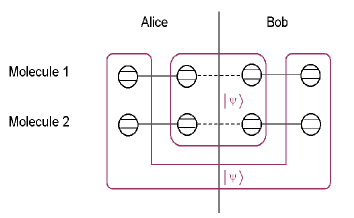
Figure 1: Creating multiple copies of an ensemble described by $|{\psi}\rangle$. $N=2$ and $M^{\prime}=4$, which means that Alice and Bob share two copies of the $N=2$, $M=2$ ensemble.

IV Applications of $S_{N}$-SSR

IV.1 Asymptotic Loss of Entanglement

Typically with the $S_{N}$-SSR applied to many identical copies of an entangled state the amount of extractable entanglement will be less than in the unconstrained case. This was actually done first by Eisert et al.  Eis00 . Consider an ensemble of $N=2J$ identically prepared molecules each consisting of two nuclei in the following state:

$$|{\psi}\rangle=\alpha|{\downarrow_{A}\downarrow_{B}}\rangle+\beta|{\uparrow_{A}\uparrow_{B}}\rangle,$$ (31)

where $\alpha$ and $\beta$ can be taken to be real, so that $\alpha^{2}+\beta^{2}=1$ is the normalization condition. Using the Hilbert space decomposition into permutation and angular momentum subspaces from Sec. III.3.1, the total state of the ensemble can be written as,

$$|{\psi}\rangle^{\otimes N} = \sum_{j=J-\lfloor J\rfloor}^{J}\sum_{n=1}^{d_{j}}\sum_{m=-j}^{j}\alpha^{J-m}\beta^{J+m}$$ (32)

$$\times|{j,n}\rangle_{A}|{j,m}\rangle_{A}\,\otimes\,|{j,n}\rangle_{B}|{j,m}\rangle_{B},$$

where the condition $\alpha^{2}+\beta^{2}=1$ also indicates that $|{\psi}\rangle^{\otimes N}$ is normalized. From the spin representation [Eq. (31)] it is easy to see that the entanglement for the ensemble is $E(|{\psi}\rangle^{\otimes N})=N(-\alpha^{2}\log\alpha^{2}-\beta^{2}\log\beta^{2})=NE(|\psi\rangle)$.

We now consider the amount of extractable entanglement under the $S_{N}$-SSR. To do so, we must take into account the effect of the SSR on the ensemble state. The permutation operator ${\cal P}$ results in a completely mixed state for both Alice and Bob in the permutation subspace. That is,

$$|{\psi}\rangle^{\otimes N}\!\!\! \stackrel{{\scriptstyle{\cal P}_{A}\otimes{\cal P}_{B}}}{{\longrightarrow}}\ \ \sum_{j=J-\lfloor J\rfloor}^{J}\;\sum_{n=1}^{d_{j}}\ \frac{I_{A}^{j}}{d_{j}}\otimes\frac{I_{B}^{j}}{d_{j}}$$ (33)

$$\otimes \!\!\left(\uplus\sum_{m=-j}^{j}\alpha^{J-m}\beta^{J+m}|{j,m}\rangle_{A}|{j,m}\rangle_{B}\right)\!\!,$$

where implementation of the $S_{N}$-SSR has also destroyed coherence between different $j$ terms. Note that $I_{A}^{j}$ is the identity operator on the Hilbert space $\mathbb{M}_{j}$ for Alice, and similarly $I_{B}^{j}$ for Bob. Eq. (33) can be simplified by defining the (normalized) angular momentum part of the state as $|{\phi_{j}}\rangle=(1/\sqrt{d_{j}\wp_{j}}\ )\sum_{m=-j}^{j}\alpha^{J-m}\beta^{J+m}|{j,m}\rangle_{A}\otimes|{j,m}\rangle_{B}$. The term $\wp_{j}=\sum_{m=-j}^{j}\alpha^{2(J-m)}\beta^{2(J+m)}/d_{j}$ is the probability of obtaining the $j$th angular momentum value and a particular irrep, indexed by $n_{A}$ and $n_{B}$. Since there are actually $d_{j}^{2}$ irreps for each $j$ value, the probability of obtaining a particular $j$ is $d_{j}^{2}\wp_{j}$. It can be verified that $\sum_{j=J-\lfloor J\rfloor}^{J}d_{j}^{2}\wp_{j}=1$ as required by conservation of probability. Using these definitions allows Eq. (33) to be rearranged as,

$${\cal P}_{A}\! \otimes \!{\cal P}_{B}\ \left(|{\psi}\rangle\langle{\psi}|\right)^{\otimes N}$$ (34)

$$= \sum_{j=J-\lfloor J\rfloor}^{J}\;\!\!\!\!\!d_{j}\left(\frac{I_{A}}{d_{j}}\otimes\frac{I_{B}}{d_{j}}\right)\otimes\ d_{j}\wp_{j}\left(\frac{}{}\!\!\uplus|{\phi_{j}}\rangle\right)\!.$$

For convenience we will omit writing the completely mixed states on the permutation subspace, although when we write the $S_{N}$-invariant state they are assumed to be there. Using this convention, the $S_{N}$-invariant state can be written compactly as

$${\cal P}_{A}\otimes{\cal P}_{B}\left(|{\psi}\rangle\langle{\psi}|\right)^{\otimes N}=\sum_{j=J-\lfloor J\rfloor}^{J}\;d_{j}^{2}\wp_{j}\ \left(\!\!\frac{}{}\uplus|{\phi_{j}}\rangle\right)\!.$$ (35)

Since no observed quantities can be changed by replacing $|{\psi}\rangle^{\otimes N}$ with the $S_{N}$-invariant state, calculating the constrained entanglement of $|{\psi}\rangle^{\otimes N}$ is equivalent to

$$E_{S_{N}\textrm{-SSR}}(|{\psi}\rangle^{\otimes N})=E_{D}\left({{\cal P}_{A}\otimes{\cal P}_{B}\left(|{\psi}\rangle\langle{\psi}|\right)^{\otimes N}}\right).$$ (36)

If the state of interest is composed of states that are are locally distinguishable (for both Alice and Bob) then it is known as a biorthogonal mixture (see Ref. Herbut03 for more details). The expected entanglement of such a state is simply a weighted sum of the entanglement present in each of the the possible states. That is,

$$E(\rho)=\wp_{1}E(\rho_{1})+\wp_{2}E(\rho_{2})+\ldots,$$ (37)

where $E(\rho_{1,2,\ldots})$ is the entanglement of the locally distinguishable states making up the mixture, and $\wp_{1,2,\ldots}$ are the corresponding probabilities of each state occurring. The $S_{N}$-invariant state is of this form, with $\uplus|{\phi_{j}}\rangle$ the possible states and $d_{j}^{2}\wp_{j}$ the corresponding probabilities. Therefore, Eq. (36) can be rewritten as

$$E_{S_{N}\textrm{-SSR}}(|{\psi}\rangle^{\otimes N})=\sum_{j=J-\lfloor J\rfloor}^{J}d_{j}^{2}\wp_{j}E(|{\phi_{j}}\rangle),$$ (38)

where $E(|{\phi_{j}}\rangle)$ is the entanglement of the angular momentum state $|{\phi_{j}}\rangle$. We expect the total amount of constrained entanglement to be less than the $E(|{\psi}\rangle^{\otimes N})=N(-\alpha^{2}\log\alpha^{2}-\beta^{2}\log\beta^{2})$ ebits calculated for the unconstrained system.

To demonstrate this, consider the particular case of Bell states, where $\alpha=\beta=\mbox{$\frac{1}{\sqrt{2}}$}$. This gives $E(|{\psi}\rangle^{\otimes N})=N$, but, as shown by Bartlett and Wiseman BarWis03 ,

$$E_{S_{N}\textrm{-SSR}}(|{\psi}\rangle^{\otimes N}) = \!\!\!\!\sum_{j=J-\lfloor J\rfloor}^{J}\!\!d_{j}^{2}\wp_{j}\log_{2}(2j+1).$$ (39)

This expression can be simplified significantly in the asymptotic limit (i.e. $J=N/2\rightarrow\infty$) because the probability distribution $d_{j}^{2}\wp_{j}$ becomes sharply peaked at a single $j$ value. Thus, a single term in the sum essentially determines the value of the entanglement. It can be shown that for large ensembles ($N\gg 1$) the significant term in the sum is specified by $j\approx\sqrt{J}$. This means that in the asymptotic limit Eq. (39) reduces to approximately $(1/2)\log_{2}N$. Since this is the maximum total entanglement, the entanglement per molecule must always $\to 0$ as $N\to\infty$. Hence, under the $S_{N}$-SSR for an ensemble of maximally entangled pure states we asymptotically lose the ability to access the entanglement.

IV.2 Asymptotic Recovery of Entanglement

We have just shown that under the $S_{N}$-SSR we apparently ‘lose’ much of the entanglement in the ensemble. This might seem contrary to the intuition obtained from the U(1) case, for example, where in the limit of a large number of particles, the entanglement per particle is recovered asymptotically approaching the unconstrained entanglement WisVac03 . This discrepancy arises from taking an inappropriate form of the asymptotic limit for the $S_{N}$-SSR. As explained in Sec. III.4, having multiple copies under an $S_{N}$-SSR does not mean changing $N$. The asymptotic limit for the number of copies thus should be considered with $N$ fixed.

We begin by considering an ensemble of $N=2$ molecules. As discussed in Sec. III.3.2 this is a special case that considerably simplifies the action of $\mathcal{P}$. To relate to Sec. IV.1, imagine that Alice and Bob share an ensemble of two molecules each of which is a Bell state. The difference here is that we allow each molecule to be larger and to contain $C$ copies of a Bell state. That is, we allow Alice and Bob to share $C$ copies of the original $N=2$ ensemble.

For convenience we define the density matrix for $C=1$ copy of the ensemble of $N=2$ Bell states as

$$\rho_{AB}=\Big{[}|{\psi^{-}}\rangle\langle{\psi^{-}}|\Big{]}^{\otimes 2},$$ (40)

where the Bell singlet state is defined as $|{\psi^{-}}\rangle=\frac{1}{\sqrt{2}}(|{\uparrow_{A}\downarrow_{B}}\rangle-|{\downarrow_{A}\uparrow_{B}}\rangle)$. The state $\rho_{AB}$ can also be expressed as

$$\rho_{AB} = \uplus\frac{1}{2}\Big{[}|{A}\rangle+\sqrt{3}|{S}\rangle\Big{]},$$ (41)

where we define normalised states in the antisymmetric and symmetric subspaces in terms of the $|{j,m}\rangle$ basis (recall Sec. III.3.1) as $|{A}\rangle=|{j=0,m=0}\rangle_{A}|{j=0,m=0}\rangle_{B}$ and $|{S}\rangle=(1/\sqrt{3})\sum_{m=-1}^{1}|{j=1,m}\rangle_{A}|{j=1,-m}\rangle_{B}$ respectively.

Using this representation for the state, it becomes apparent that $\mathcal{P}$ simply destroys coherence between the symmetric and antisymmetric subspaces which can be represented as

$$\mathcal{P}\rho_{AB}=\uplus\sqrt{\frac{1}{4}}|{A}\rangle\uplus\sqrt{\frac{3}{4}}|{S}\rangle.$$ (42)

Since Alice and Bob share a biorthogonal mixture, they can each make local measurements to distinguish between the symmetric and antisymmetric subspaces. This is equivalent to the situation considered by Eisert et al. Eis00 . With probability $1/4$ they find that they have the locally antisymmetric state and they retain no entanglement (as this is a separable state). However, with probability $3/4$ they obtain the locally symmetric state, which is equivalent to a maximally entangled qutrit state. In that case they retain $\frac{3}{4}\log_{2}(3)\approx 1.19$ ebits of entanglement. Without the $S_{2}$-SSR constraining their two Bell states, Alice and Bob would possess 2 ebits of entanglement.

One might expect that by using the concept of multiple copies it would be possible to ameliorate the effect of the SSR. This is indeed the case, as we now show. For the $S_{2}$-SSR to apply, Alice and Bob must share entanglement contained in 2 molecules. In the simplest case, each molecule is simply a Bell singlet state and the combined state is $\rho_{AB}$, as discussed above. To apply the concept of multiple copies, Alice and Bob must share $C$ copies of $\rho_{AB}$ (see Fig. 2). With no restrictions in place Alice and Bob would share $2C$ ebits of entanglement.

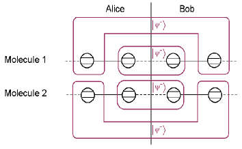
Figure 2: Two copies ($C=2$) of $\rho_{AB}$ (which is composed of two Bell states $|{\psi^{-}}\rangle$). Each molecule can be extended to include more Bell states to increase the number of copies $C$ of $\rho_{AB}$.

The calculation of how much entanglement is retained using multiple copies can be significantly simplified by noting that in this case, each of the molecules (containing $C$ Bell pairs) can be considered as a maximally entangled qudit pair. This is possible due to the global symmetry of the ensemble state chosen. In this case, each molecule can be described as a maximally entangled pair of qudits, with the qudits dimension given by $d=2^{C}$. This simplifies calculations, as the maximum entanglement of a pair of entangled qudits is readily calculated to be $E_{\rm max}=\log_{2}d$. Thus, without considering the $S_{2}$-SSR constraint, the total entanglement for the two maximally entangled qudit pairs is $E=2C$ ebits, as already derived.

We can express the state of $C$ copies of $\rho_{AB}$ under the $S_{2}$-SSR explicitly as a biorthogonal mixture of a locally symmetric and a locally antisymmetric state,

$$\mathcal{P}\left(\rho_{AB}\right)^{\otimes C}=\wp_{s}\rho_{s}+\wp_{a}\rho_{a},$$ (43)

where the weightings $\wp_{s}$ and $\wp_{a}$ are the probabilities of both Alice and Bob obtaining a locally symmetric or locally antisymmetric state respectively. These probabilities depend upon the dimension of the subspace that each of the local states occupy: $\wp_{s}={\rm dim}\left(\mathbb{Q}_{s}\right)/d^{2}$ and $\wp_{a}={\rm dim}\left(\mathbb{Q}_{a}\right)/d^{2}$ (recall the expressions for the subspace dimensions defined in Sec. III.3.2).

The structure of Eq. (43) means that it is quite straightforward to calculate the extractable entanglement of $\left(\rho_{AB}\right)^{\otimes\ C}$. It is simply a weighted average of the entanglement in the two subspaces:

$$E=\frac{d^{2}-d}{2d^{2}}\log_{2}\!\!\left(\frac{d^{2}-d}{2}\right)+\frac{d^{2}+d}{2d^{2}}\log_{2}\!\!\left(\frac{d^{2}+d}{2}\right).$$ (44)

For a large number of copies ($C\gg 1$ ) the dimension $d$ is large and Eq. (44) reduces to approximately $E=2C-1$. Thus in the asymptotic limit, nearly all of the entanglement has been recovered (only a single ebit has been lost).

Another way to consider this problem is that Alice and Bob share many copies of the state $\rho_{AB}$ via a channel (see Fig. 3). The channel is deterministic and either does nothing or performs a swap of the molecules. If Alice and Bob were unable to make collective measurements on their entire collection of qubits then they could still make use of their copies of $\rho_{AB}$ to asymptotically retain much of their entanglement. A non-optimal procedure that they could implement would be to use up a small number of copies to find out what map the channel performs (either identity or swapping). Once they know what the channel does they can then safely use the 1 ebit of entanglement in each of their remaining Bell pairs. This method is non-optimal because Alice and Bob lose at least a few ebits of entanglement in characterizing the channel (and asymptotically with collective measurements they need lose only 1 ebit).

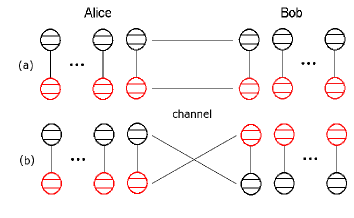
Figure 3: Alice and Bob share $N$ copies of $\rho_{AB}$ via a channel. In case (a) the channel distributes the states in order. In (b) the channel swaps the ordering within each pair.

In general for the case of the $S_{N}$-SSR with $N>2$ it is difficult to optimally calculate the exact asymptotic amount of entanglement recovered. However, considering the non-optimal procedure just discussed it is intuitive that Alice and Bob could recover most of their entanglement (in the asymptotic limit) simply by using up some copies of the state to characterize the ‘channel’. They would then retain the entanglement in the remaining copies. As the size of the ensemble ($N$) increases, more copies of the state will be required to satisfactorily characterize the ‘channel’ and thus more entanglement will be lost.

V Reference Frames

In general, a reference frame for a SSR is something that removes its effect. For example, a perfect reference frame completely removes the effect of, or ‘lifts’, the SSR. This is the ideal case, although in practice it is possible to have partial reference frames which only partially remove the effect of the SSR.

Usually a reference frame is an extra system added to the system of interest which allows access to degrees of freedom otherwise unaccessible due to the SSR. Thus, for an ensemble of molecules, for which the $S_{N}$-SSR applies, one might naively expect to add an extra ensemble of molecules to act as a reference frame. However, as discussed in Sec. III.4, due to the nature of the $S_{N}$ group, adding molecules would in fact alter the SSR for the system. That is, the reference molecules would actually be permuted with the system molecules, making it more, not less, difficult to gain information about the system.

Instead, the type of reference frame needed for an ensemble system is analogous to a labelling. Classically, one would think of physically writing a label (say a number) on each object, to serve as a reference ordering. Physically this corresponds not to adding molecules to the ensemble, but adding an extra nucleus (or group of nuclei) to each molecule in the ensemble.

To illustrate this, consider a simple example, with $N=3$ molecules. In this instance a pure state [where the three molecules happen to be uncorrelated, see Fig. (4)] with a reference frame is

$$|{\Psi}\rangle=|{\psi^{1},1}\rangle|{\psi^{2},2}\rangle|{\psi^{3},3}\rangle=|{\psi^{1},\psi^{2},\psi^{3}}\rangle\otimes{|{1,2,3}\rangle}$$ (45)

Here $|{\psi^{k}}\rangle$ is the state of the $M$ nuclei in the $k$th molecule (not including the reference frame) which we have assumed to factorize. In regards to the tensor product structure it is important to remember that the second system is not in the same state as the first (it need not even have the same Hilbert space dimension).

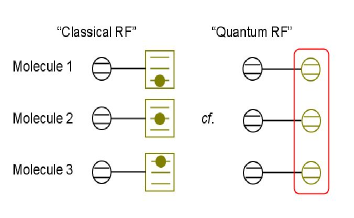
Figure 4: Classical versus quantum reference frames. The classical reference frames on the left are represented by boxes and are uncorrelated. On the right the reference frames are quantum systems and we allow for correlations between the label systems.

V.1 Quantum reference frames

In the classical example above, we placed each $N$-dimensional attached label system (nucleus or group of nuclei) in a unique product state. An obvious question is whether or not it is possible to use label systems of smaller dimension if we allow entanglement between the states of the $N$ label systems. As demonstrated by von Korff and Kempe vKK04 , it is indeed possible to reduce the dimension of the label systems by a constant factor in the limit $N\rightarrow\infty$.

Recalling the structure of the Hilbert space from Sec. III.3, a state of the $N$ label systems $|0\rangle\in(\mathbb{C}_{d})^{\otimes N}$ that works as a perfect quantum reference frame would satisfy the property that the $N!$ states

$$|p_{n}\rangle=\hat{T}(p_{n})|p_{0}\rangle\,,$$ (46)

for all $p_{n}\in S_{N}$ satisfy $|\langle p_{n}|p_{n^{\prime}}\rangle|^{2}=\delta_{n,n^{\prime}}$. This property ensures that every different ordering is classically distinguishable (i.e., is associated with an orthogonal quantum state). So the problem reduces to the following: What is the minimum $d$ such that such a set of orthogonal states exists?

First, we note that the space $\mathbb{H}_{R}$ spanned by $\{|p_{n}\rangle,\,p_{n}\in S_{N}\}$ is $N!$-dimensional and that the representation $\hat{T}$ when restricted to this space is isomorphic to the (left) regular representation. (The regular representation $R$ of a group $G$ has $G$ as a carrier space, and acts as $R(g)g^{\prime}=gg^{\prime}$.) It is well-known (Ful91 , p. 17) that the regular representation of $S_{N}$ contains every irrep $\hat{T}_{y}$ of $S_{N}$, each with a multiplicity equal to $D_{y}$, the dimension of $\hat{T}_{y}$. Thus, for $\hat{T}$ to contain the regular representation, it must contain every irrep $\hat{T}_{y}$ of $S_{N}$ with a multiplicity of at least $D_{y}$. In particular, this must hold true for the fully-antisymmetric representation of $S_{N}$ (the irrep labeled by a Young diagram consisting of a single column of $N$ boxes), and $\hat{T}$ only contains the fully-antisymmetric representation if $d\geq N$. Thus, if we demand that the label systems act as a perfect reference frame for $S_{N}$, then each label system must be at least $N$-dimensional.

However, von Korff and Kempe vKK04 have shown that it is possible to use label systems with any dimension $d>\lfloor N/e\rfloor$ if the requirement of a perfect reference frame is relaxed to the less-stringent demand that, for $p_{n}\neq p_{n^{\prime}}$, $|\langle p_{n}|p_{n^{\prime}}\rangle|^{2}\rightarrow 0$ as $N\rightarrow\infty$. (That is, that the reference frame states are distinguishable only in the asymptotic limit.) The basic idea is that if $d>\lfloor N/e\rfloor$ then, although $\hat{T}$ does not contain all irreps of $S_{N}$ with the required multiplicity, the set that are missing has measure approaching zero as $N\rightarrow\infty$. We refer the reader to vKK04 for details.

We now explicitly construct states of the form of Eq. (46), using the general construction of KMP04 that was subsequently applied specifically to the $S_{N}$ group in vKK04 . Let $\overline{Y}$ be the set of irreps that are contained in $\hat{T}$ and have sufficient multiplicity, i.e., that satisfy $\text{dim}\mathbb{Q}_{y}\geq D_{y}$. For each $y\in\overline{Y}$, choose an arbitrary subspace $\mathbb{Q}^{\prime}_{y}\subset\mathbb{Q}_{y}$ of dimension $D_{y}$. Let $\{|y,i,j\rangle,i,j=1,\ldots,D_{y}\}$ be a basis for $\mathbb{M}_{y}\otimes\mathbb{Q}^{\prime}_{y}$, where $i$ labels a basis for $\mathbb{M}_{y}$ and $j$ labels a basis for $\mathbb{Q}^{\prime}_{y}$. Define $D=\sum_{y}D_{y}^{2}$. Then the state

$$|p_{0}\rangle=\sum_{y\in\overline{Y}}\sum_{i=1}^{D_{y}}\sqrt{\frac{D_{y}}{D}}|y,i,i\rangle\,,$$ (47)

can be used to define a set of states $\{|p_{n}\rangle=\hat{T}(p_{n})|p_{0}\rangle\}$ for $p_{n}\in S_{N}$ as in Eq. (46). As demonstrated in vKK04 , $\lim_{N\to\infty}D=N!$ and $\lim_{N\to\infty}|\langle p_{n}|p_{n^{\prime}}\rangle|^{2}=\delta_{n,n^{\prime}}$ provided that $d>\lfloor N/e\rfloor$.

V.2 Shared reference frames

The simplest shared reference frame is for Alice and Bob each to have a reference frame. In general, if Alice and Bob share $N$ tensor product states and both have a reference frame for each state, then the total system can be described as

$$|{\Psi}\rangle = \bigotimes_{i=1}^{N}|{\psi^{i}_{AB},i_{A},i_{B}}\rangle.$$ (48)

For example, this can be written out explicitly for the case when two product states are shared,

$$|{\Psi}\rangle = |{\psi^{1}_{AB},1_{A},1_{B}}\rangle|{\psi^{2}_{AB},2_{A},2_{B}}\rangle$$ (49)

$$= |{\Psi_{AB}}\rangle|{p_{0}}\rangle_{A}|{p_{0}}\rangle_{B},$$

where in the second line we have written the shared states first, followed by Alice and Bob’s reference frames. Note that we have rewritten Alice’s reference state $|{\cdots,1_{A},\cdots}\rangle|{\cdots,2_{A},\cdots}\rangle$ as the fiducial reference state $|{\cdots}\rangle|{p_{0}}\rangle_{A}|{\cdots}\rangle_{B}$, and similarly for Bob’s.

Although these states are separable, they cannot be prepared locally by ${\cal P}_{A}\otimes{\cal P}_{B}$-invariant operations from a ${\cal P}_{A}\otimes{\cal P}_{B}$-invariant state. Hence they are bound entangled states which may become locally preparable. (Recall the definitions in Sec. II.3.) Note that such states are not globally ${\cal P}$-invariant. However, using the final reference frame basis above we can write a separable ${\cal P}$-invariant reference frame:

$${\biguplus_{p_{n}\in S_{N}}\frac{1}{\sqrt{N!}}|{p_{n}}\rangle_{A}|{p_{n}}\rangle_{B}}.$$ (50)

This reference frame is an incoherent mixture of reference states which is an example of a shared reference frame. The key point is that the same permutation is applied to both Alice and Bob’s reference states resulting in perfect correlation between each of Alice and Bob’s labels. That is, this reference frames gives no indication of labels for individual states, but indicates that Alice and Bob’s particles are in the same order. States of this form are mixed (separable) and hence not part of the classification scheme of Sec. II.3.

Alternatively, a pure globally ${\cal P}$-invariant reference frame can be constructed by considering non-separable states:

$${\sum_{p_{n}\in S_{N}}\frac{1}{\sqrt{N!}}|{p_{n}}\rangle_{A}|{p_{n}}\rangle_{B}}.$$ (51)

This state is a coherent superposition of reference states which are perfectly correlated between Alice and Bob. Once again for an explicit example we consider a reference frame for the $S_{2}$ group

$$|{\Psi}\rangle_{\rm RF} = \frac{1}{\sqrt{2}}\sum_{p_{n}\in S_{2}}|{p_{n}}\rangle_{A}|{p_{n}}\rangle_{B}$$ (52)

$$= \frac{1}{\sqrt{2}}\left[|{p_{0}}\rangle_{A}|{p_{0}}\rangle_{B}+|{p_{1}}\rangle_{A}|{p_{1}}\rangle_{B}\right],$$

where $p_{0}$ is the identity permutation and $p_{1}$ is the swap permutation. In this case it can be shown that the partial transpose of the state matrix $\rho_{\rm RF}=|{\Psi}\rangle_{\rm RF}\langle{\Psi}|_{\rm RF}$ is actually equal to $\rho_{\rm RF}$. Thus it is a valid state matrix which means that $\rho_{\rm RF}$ has a positive partial transpose Peres96 . This shows that for the $S_{2}$ group, which is actually an Abelian group, a shared reference state of the form of Eq. (52) is become 1-distillable (this is because it contains no entanglement under the $S_{2}$-SSR but becomes 1-distillable if the SSR is lifted).

VI Analogies with mixed-state entanglement

VI.1 Activation

Recall from section II.1.2 that a general state $\rho$ is called 1-distillable if by LOCC Alice and Bob can, with some probability, create from it a nonseparable two-qubit state. Also recall that there are bound entangled states that become 1-distillable when the two parties have their LOCC supplemented by a shared PPT-channel. These states, as we have mentioned in section II.1.3, are called become 1-distillable states.

Since $S_{N}$ is a finite group, reference frames for the $S_{N}$ group can be finite (this is quite different to the case for Lie group SSRs such as the U(1)-SSR). Moreover, the $S_{N}$ reference frames can be used without being disturbed because they form an orthonormal set. Thus under the $S_{N}$-SSR there is no distinction between activation of a bound entangled state (by a bound entangled state which becomes locally preparable) and lifting the $S_{N}$-SSR to make become 1-distillable states 1-distillable.

Activation of a bound entangled state can be seen in the following example. If $N=2$ and $M=2$, (i.e Alice and Bob own one nucleus per molecule), then the state

$${\sqrt{2}|{\psi}\rangle=|{+}\rangle_{A}|{-}\rangle_{B}+|{-}\rangle_{A}|{+}\rangle_{B}},$$ (53)

is bound entangled that can become 1-distillable. Here $|{+}\rangle=|{j=1,m=0}\rangle$ and $|{-}\rangle=|{j=0,m=0}\rangle$, so ${\hat{T}(p_{1})|{\pm}\rangle=\pm|{\pm}\rangle}$. From this it is easy to see that $|{\psi}\rangle$ is globally symmetric, but under the local SSR,

$${\sqrt{2}|{\psi}\rangle\stackrel{{\scriptstyle{\cal P}_{A}\otimes{\cal P}_{B}}}{{\longrightarrow}}\;\uplus\;|{+}\rangle_{A}|{-}\rangle_{B}\;{\uplus}\;|{-}\rangle_{A}|{+}\rangle_{B}},$$ (54)

which is clearly separable. Hence, with the SSR the state has no distillable entanglement.

It is possible to completely lift the SSR and regain 1-ebit of entanglement from this state. This is achieved by adding an extra shared state $|{\phi}\rangle$ to activate the bound entanglement in $|{\psi}\rangle$. This is shown in Fig. 5. For instance, the simplest perfect reference frame $|{\phi}\rangle$ would label each of Alice and Bob’s nuclei, for example, $|{\phi}\rangle=|{1_{A},2_{A}}\rangle|{1_{B},2_{B}}\rangle=|{p_{0}}\rangle_{A}|{p_{0}}\rangle_{B}$. Then it becomes possible for Alice to find out which of her nuclei is correlated with which of Bob’s simply through measurement of the shared reference state. Thus by use of a reference frame (that is, activating the bound entanglement), it is possible to access 1-ebit of entanglement from the become 1-distillable state.

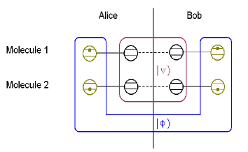
Figure 5: Using an extra state $|{\phi}\rangle$ to activate the bound entanglement in $|{\psi}\rangle$. In this case $|{\phi}\rangle$ acts as a perfect reference frame and all the entanglement in $|{\psi}\rangle$ is recovered.

VI.2 Distillation

We now illustrate the phenomenon of distillation using the same example state $|{\psi}\rangle$. That is, although without a reference frame the state ${\sqrt{2}|{\psi}\rangle=|{+}\rangle_{A}|{-}\rangle_{B}+|{-}\rangle_{A}|{+}\rangle_{B}}$ has $E_{S_{2}\textrm{-SSR}}=0$, with two copies some entanglement can be obtained.

Recall from Section III.4 that two copies does not mean four molecules. Since $S_{2}$ is fixed, we still have $N=2$ molecules, but instead of $M=2$ we now have $M^{\prime}=4$, that is, Alice and Bob each have two nuclei per molecule. This is demonstrated in Fig. 6.

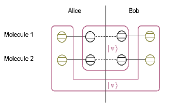
Figure 6: With two copies of the state $|{\psi}\rangle$ the second can act as a reference frame for the first allowing one ebit of entanglement to be accessed. This is considered an imperfect reference frame for the system as we would expect two copies of $|{\psi}\rangle$ to contain two ebits of entanglement.

The state for the two copies can be written as,

$$(\sqrt{2}|{\psi}\rangle)^{\otimes 2} = |{++}\rangle_{A}|{--}\rangle_{B}+|{-+}\rangle_{A}|{+-}\rangle_{B}$$ (55)

$${+}\,|{+-}\rangle_{A}|{-+}\rangle_{B}+|{--}\rangle_{A}|{++}\rangle_{B},$$

which with a perfect reference frame contains two ebits of entanglement. The effect of the SSR is to create a mixture of the unchanged state with the state formed by applying the swap $\hat{T}(p_{1})$ to Alice’s particles (or Bob’s). Thus under the $S_{2}$-SSR, the state becomes,

$$(\sqrt{2}|{\psi}\rangle)^{\otimes 2} \stackrel{{\scriptstyle{\cal P}_{A}\otimes{\cal P}_{B}}}{{\longrightarrow}} \uplus\left(|{++}\rangle_{A}|{--}\rangle_{B}+|{--}\rangle_{A}|{++}\rangle_{B}\right)$$ (56)

$${\uplus}\,\left(|{-+}\rangle_{A}|{+-}\rangle_{B}+|{+-}\rangle_{A}|{-+}\rangle_{B}\right).$$

Now Alice and Bob share a mixture of two superpositions. By Alice and Bob each measuring a suitable observable (such as $\hat{O}=\uplus|{++}\rangle\uplus|{--}\rangle$ for example), they can perform a local measurement to discriminate the two superposition states superpositions they actually (without destroying the superposition). Thus they have access to 1 ebit of constrained entanglement. In this case we started with two copies of $|{\psi}\rangle$, therefore with a perfect reference frame we would expect to be able to recover two ebits of entanglement. However, even without an external reference frame it is possible to access entanglement from two copies of the state. This is because one of the states acts a reference for the other, activating its entanglement. Alternatively, one could consider that each of the entangled states acts a as partial reference frame for the other, allowing half of its entanglement to be accessed. This is an example of a case where no entanglement could be distilled from a single copy of the state (with no reference frame), but two copies of the state allows entanglement to be distilled. Hence the state $|{\psi}\rangle$ is not 1-distillable, but it is 2-distillable. That is to say that this state demonstrates the fact that the 1-distillable states are a subset of the 2-distillable states for the $S_{2}$-SSR.

VII Beyond the $S_{N}$-SSR

VII.1 Adding a stronger constraint

So far we have considered the problem of describing ensemble quantum information processing using the formalism for SSRs associated with some group. The $S_{N}$-SSR says that all elements (molecules) are subject to identical operations. This constraint has a demonstrable effect on the properties of the system, which can however be removed through use of additional resources such as reference frames. We now wish to consider the case where a stronger constraint than a SSR may apply to a system.

First we point out a difference between NMR experiments and spin-squeezing experiments, for which the $S_{N}$-SSR also applies. In the latter, it is possible to perform symmetric operations which entangle the elements (atoms), such as spin-squeezing unitaries Ueda or quantum non-demolition measurements of $\hat{J}_{z}$ Kuz00 . By contrast, in NMR it is not possible to induce correlations between different molecules. The reasons for this difference are subtle, and relate to practical constraints due to decoherence during the read-out. This constraint also manifests itself in very low measurement efficiencies, but here we ignore that issue.

Consider the $M=1$ case for simplicity. Then all that can be done in practice in NMR experiments is

• Rotations $\exp(-i\underline{\theta}\cdot\underline{\hat{J}})=\exp(-i\underline{\theta}\cdot\sum_{k=1}^{N}\underline{\hat{\sigma}}^{k}/2)$.

• Destructive measurement of $\hat{J}_{z}=\sum_{k=1}^{N}\hat{\sigma}_{z}^{k}/2$.

Here $\underline{\hat{\sigma}}^{k}$ denotes $I\otimes\ldots I\otimes\underline{\hat{\sigma}}\otimes I\ldots\otimes I$ with $\underline{\hat{\sigma}}$ in the $k$th position. When making a measurement of this type (e.g. measuring $\hat{J}_{z}$) we actually get out an overall signal which is proportional to the sum of the spin ($\hat{\sigma}_{z}$) for each particle. Moreover, the final state of the ensemble is unrelated to the measurement result, due to thermal decoherence. Thus in general, the only operations possible in NMR are to make destructive measurements of symmetric observables that are additive over the ensemble:

$$\hat{O}_{\rm total}=\sum_{k}\hat{O}^{k},$$ (57)

where $\hat{O}^{k}$ is the operator for the $k$th particle as above. We call such operations non-collective. This terminology is appropriate because the result of the measurement could be obtained by individually measuring each element of the ensemble and summing the results.

We can contrast such non-collective operations with a collective operation like measuring (destructively or otherwise) $\hat{J}^{2}$ to find out the value of the total angular momentum $j$ for the ensemble. This could not be done by measuring each particle and summing the results. Previous work using the $S_{N}$-SSR assumed that such collective measurements are possible. We will now consider the case where operations need not only be symmetric but also non-collective, as a stronger constraint on the system.

We suspect that we cannot completely characterize these constraints by any $G$-SSR. Instead we must supplement the $S_{N}$-SSR with the extra constraint that the operations also be non-collective. This complicates matters, as we are now unable to write down an equivalent state which is invariant under all the allowable operations. Despite this, we wish to determine if any entanglement survives under this stronger constraint.

Since we are unable to determine an operationally equivalent state matrix for the constrained state we cannot calculate the extractable entanglement directly. However, if a Bell inequality violation can be demonstrated then this proves that entanglement is present in some form. So the question becomes, using the $S_{N}$-invariant state as a description for the system, is it possible to demonstrate Bell nonlocality using non-collective operations?

VII.2 Bell inequality for ensembles

For specificity, we consider the problem of demonstrating Bell nonlocality under symmetric, non-collective measurements on an ensemble of $N=2J$ Bell singlets, $|{\psi}\rangle=|{\psi^{-}}\rangle^{\otimes N}$. As discussed in Sec. IV.1 the interesting part of this state can be written for simplicity as

$$\mathcal{P}\left[\left(|{\psi}\rangle\langle{\psi}|\right)^{\otimes N}\right]=\sum_{j=J-\lfloor J\rfloor}^{J}{d_{j}}^{2}\wp_{j}|\phi_{j}\rangle\langle\phi_{j}|,$$ (58)

which is an incoherent mixture of different spin ($j$) states. The added constraint means that we are unable to measure $\hat{J}^{2}$ directly, but can only measure components of spin (such as $\hat{J}_{z}$). Thus we must be derive a Bell inequality that allows for particles of different spin (i.e. different $j$ values).

Mermin Mer** developed a Bell inequality for spin-$j$ particles by considering a generalization of the Bohm-EPR experiment. The only assumption that needs to be satisfied for this inequality to be applicable is that the desired state exhibit perfect anticorrelation in the spins of the two particles. The inequality can be written as,

$$\left\langle\left|m_{A}(\hat{a})-m_{B}(\hat{b})\right|\right\rangle \geq \frac{1}{J}\Big{(}\langle m_{A}(\hat{a})m_{B}(\hat{c})\rangle\Big{.}$$ (59)

$$+\left.\langle m_{A}(\hat{b})m_{B}(\hat{c})\rangle\right),$$

where $m_{i}(\hat{a})$ represents the spin component of the $i$th particle in the $\hat{a}$ direction and $J$ is an upper bound on the $m_{i}(\hat{a})$. For Mermin’s case one can (and Mermin does) choose $J=j$. However, we require that the parameter $J$ because we cannot distinguish between different $j$-values. Inequality (59) will be satisfied by any theory obeying local causality. For ease of analysis we define a quantity

$$M_{J}(\theta) = \left\langle\left|m_{A}(\hat{a})-m_{B}(\hat{b})\right|\right\rangle\$$ (60)

$$-\frac{1}{J}\left(\langle m_{A}(\hat{a})m_{B}(\hat{c})\rangle+\langle m_{A}(\hat{b})m_{B}(\hat{c})\rangle\right).$$

The condition for local causality to be satisfied can thus be expressed as $M_{J}(\theta)\geq 0$.

Consider a Stern-Gerlach experiment such that the spin can be measured along one of three axes defined by coplanar vectors $\hat{a}$, $\hat{b}$, and $\hat{c}$. Mermin defined these axes such that the vectors $\hat{a}$ and $\hat{b}$ make the same angle $\pi/2+\theta$ with $\hat{c}$, and the angle $\pi-2\theta$ with each other. Using this set up for two perfectly anticorrelated spin-$j$ particles, quantum mechanics predicts that Eq. (60) can be expressed as

$$M_{J}^{\rm spin-j}(\theta)=f_{j}(\theta)-\frac{1}{J}\frac{2j}{3}\left(j+1\right)\sin\theta,$$ (61)

where the functions $f_{j}(\theta)$ are defined as

$$f_{j}(\theta)=\frac{1}{2j+1}\sum_{m,m^{\prime}}\left|m-m^{\prime}\right|\left|\langle{m}|e^{-2i\theta\hat{S}_{y}}|{m^{\prime}}\rangle\right|^{2},$$ (62)

and $\hat{S}_{y}$ is a spin matrix.

Now an ensemble of Bell singlet states is perfectly anticorrelated in spin and thus Eq. (58) satisfies the necessary assumption for inequality (59) to be applicable. Also, when Mermin evaluated Eq. (61) he assumed measurements of spin components, that is, non-collective measurements. Thus it is possible to use the same method as Mermin to evaluate the Bell inequality for an NMR ensemble, as all the relevant constraints are accounted for. The ensemble state simply behaves like an incoherent mixture of different spin-$j$ states.

Thus, for an ensemble of Bell singlet states, quantum mechanics predicts Eq. (60) can be written as

$$M_{J}^{\rm Ensemble}(\theta)=\sum_{j=J-\lfloor J\rfloor}^{J}d_{j}^{2}\wp_{j}M_{J}^{\rm spin-j}(\theta),$$ (63)

where $M_{J}^{\rm Ensemble}(\theta)<0$ demonstrates Bell-nonlocality.

VII.3 Demonstrating Bell nonlocality

We are now in a position to show that Bell-nonlocality survives under stronger constraints than those imposed by a SSR alone. To do this we must evaluate $M_{J}^{\rm Ensemble}(\theta)$ and show that it can become negative. To simplify this task it is instructive to recall the form of Eq. (61). When Mermin evaluated these terms, he found to a good approximation (particularly for large $J$) that he was able to use a quadratic form to simplify their evaluation. Using the same approximation allows $M_{J}^{\rm Ensemble}(\theta)$ to be simplified to the expression

$$M_{J}^{\rm Ensemble^{\prime}}(\theta)=\!\!\!\!\!\sum_{j=J-\lfloor J\rfloor}^{J}\!\!\!\!\!d_{j}^{2}\wp_{j}\left[\frac{2}{3}j\left(j+1\right)\sin\theta\left(2\sin\theta-\frac{1}{J}\right)\right]\!\!,$$ (64)

where the prime indicates an approximation.

Now, the probability terms $d_{j}^{2}\wp_{j}$ in Eq. (64) are always positive, so the question becomes, can the remaining factor be negative? If this factor is negative for all terms in the sum, then $M_{J}^{\rm Ensemble^{\prime}}(\theta)$ is negative and the state exhibits Bell nonlocality. Examining the terms in the sum more closely reveals that there is always a linear (in $\sin\theta$) term subtracted from a quadratic (in $\sin\theta$) term. Hence, if $\theta$ (and thus $\sin\theta$) is small enough, then the linear term will always be dominant, resulting in a negative contribution to the sum. It is possible to choose $\theta$ to be small enough that every term in the sum will be negative, thus $M_{J}^{\rm Ensemble^{\prime}}(\theta)<0$ and the ensemble state exhibits Bell nonlocality.

To put it explicitly (by solving for $\theta$ in terms of $J$) the ensemble state exhibits Bell-nonlocality despite the constraints when the detectors can be arranged to make measurements defined by $\theta$ where

$$0<\sin\theta<1/2J.$$ (65)

This is actually a lower bound on the range of $\sin\theta$ for which a violation is possible. For small values of $J$ ($\leq 3$), Eq. (63) can be explicitly calculated (without resorting to approximations). Even for these small values of $J$ the exact numerical results agree quite well with the range of angles specified by Eq. (65) and the agreement improves with larger $J$. This lends confidence that for large $J$ the approximation leading to Eq. (65) is a valid one.

Somewhat surprisingly, Eq. (65) gives exactly the same angular range for which Mermin demonstrated a pair of (unconstrained) entangled spin-$J$ particles exhibit Bell nonlocality. One may then ask which of the two systems, an ensemble of Bell states or a pair of spin-$J$ particles, violates the inequality more strongly. A way to measure this is to consider the depth of the violation, that is, how negative $M_{J}(\theta)$ becomes. For a pair of perfectly anticorrelated spin-$J$ particles, the minimum value of $M_{J}(\theta)$ converges to a constant value of $-1/12$ for large $J$. In contrast, for an ensemble of $N=2J$ Bell states, the minimum of $M_{J}^{\rm Ensemble^{\prime}}(\theta)$ scales as $-1/J$. That is, the violation depth tends to zero for large ensembles. Thus, a pair of spin-$J$ particles violates this Bell inequality more strongly than an ensemble of $2J$ Bell states under our stronger constraint.

VIII Summary

In this paper we have classified groups of states based on their mixed state entanglement properties and related these states to the well known concepts of activation and distillation. We have also reviewed the analogy between mixed state entanglement and that of pure state entanglement constrained by a SSR. In particular we have focused on the symmetric group SSR. We have demonstrated that the $S_{N}$-SSR limits the amount of entanglement that can be accessed from an ensemble of entangled states. In comparison with U(1)-SSRs such as the particle number SSR we show how to apply the correct notion of multiple copies of an ensemble state to asymptotically recover the entanglement lost due to the SSR. We have also discussed the concepts of reference frames and given examples to illustrate the similarities between concepts of activation, distillation and use of reference frames (or multiple copies of states) to recover entanglement. For the $S_{2}$-SSR we showed that by using multiple copies of the ensemble, it is possible to only lose 1 ebit of entanglement (asymptotically).

Finally we gave an example where it does not seem possible to formulate the constraints on a system as a SSR. This situation arises naturally in the context of a liquid NMR ensemble. The lack of individual addressability requires that the $S_{N}$-SSR be considered. However, other technical constraints arise due to the large amount of thermal noise present in NMR ensembles. This noise manifests itself in two ways: low measurement efficiency and the fact that only non-collective measurements are possible. We addressed the latter manifestation and went on to show that despite this stronger constraint it is still possible in principle to demonstrate Bell nonlocality. It may prove interesting to attempt also to include the effect of the low efficiency constraint.

Further studies of physical constraints which cannot be formalized as SSRs may prove a fruitful area of research, not only for explaining experiments but also for understanding the properties of entanglement in general.

- (1) M. A. Nielsen and I. L. Chuang, Quantum Computation and Quantum Information (Cambridge University Press, Cambridge, 2000).
- (2) M. Horodecki, P. Horodecki and R. Horodecki, in Quantum Information: An Introduction to Basic Theoretical Concepts and Experiments, Vol. 173 of Springer Tracts in Modern Physics ed. G. Alber et al. (Springer Verlag, Berlin, 2001), pp. 151-195.
- (3) H. Barnum, E. Knill, G. Ortiz, and L. Viola, Phys. Rev. A 68, 032308 (2003).
- (4) H. Barnum, E. Knill, G. Ortiz, R. Somma, and L. Viola, Phys. Rev. Lett. 92, 107902 (2004).
- (5) A. Kitaev, D. Mayers and J. Preskill, Phys. Rev. A69, 052326 (2004).
- (6) S. D. Bartlett and H. M. Wiseman, Phys. Rev. Lett. 91, 097903 (2003).
- (7) J. A. Vaccaro, F. Anselmi, H. M. Wiseman, and K. Jacobs, quant-ph/0501121 (unpublished).
- (8) S. D. Bartlett, A. C. Doherty, R.W. Spekkens, and H. M. Wiseman, Phys. Rev. A 73, 022311 (2006).
- (9) F. Verstraete and J. I. Cirac, Phys. Rev. Lett. 91, 010404 (2003).
- (10) H. M. Wiseman and J. A. Vaccaro, Phys. Rev. Lett. , 91, 097902 (2003).
- (11) N. Schuch, F. Verstraete, and J. I. Cirac, Phys. Rev. A 70, 042310 (2004).
- (12) H. M. Wiseman, J. Opt. B. 6, S849-S859 (2004).
- (13) B. C. Sanders, S. D. Bartlett, T. Rudolph, and P. L. Knight, Phys. Rev. A 68, 042329 (2003).
- (14) T. Rudolph and B. C. Sanders, Phys. Rev. Lett. 87, 077903 (2001).
- (15) S. J. van Enk and C. A. Fuchs, Phys. Rev. Lett. 88, 027902 (2002).
- (16) J. von Korff and J. Kempe, Phys. Rev. Lett. 93, 260502 (2004).
- (17) J. S. Bell, Physics (New York) 1, 195 (1964).
- (18) E. Schrödinger, Naturwissenschaften 23, 807 (1935); English translation by J. D. Trimmer in Proc. Am. Philosophical Soc. 124, 323 (1980).
- (19) E. Schrödinger, Proc. Camb. Phil. Soc. 32, 446 (1936).
- (20) R. F. Werner, Phys. Rev. A40, 4277 (1989).
- (21) C. H. Bennett et al., Phys. Rev. Lett. 76, 722 (1996); C. H. Bennett, D. P. DiVincenzo, J. A. Smolin and W. K. Wootters, Phys. Rev. A54, 3824 (1996).
- (22) M. Horodecki, P. Horodecki and R. Horodecki, Phys. Rev. Lett. 80, 5239 (1998).
- (23) L. Gurvits, quant-ph/0201022 (unpublished).
- (24) A. C. Doherty, P. A. Parrilo, and F. M. Spedalieri, Phys. Rev. Lett. 88, 187904 (2002).
- (25) D. P. DiVincenzo, P. W. Shor, J. A. Smolin, B. M. Terhal and A. V. Thapliyal, Phys. Rev. A61, 062312 (2000).
- (26) W. Dür, J. I. Cirac, M. Lewenstein and D. Bruß, Phys. Rev. A61, 062313 (2000).
- (27) M. Horodecki, P. Horodecki and R. Horodecki, Phys. Rev. Lett. 78, 574 (1997).
- (28) J. Watrous, Phys. Rev. Lett. 93, 010502 (2004).
- (29) E. M. Rains, IEEE Trans. Inf. Theory 47, 2921 (2001).
- (30) T. Eggeling, KGH. Vollbrecht, R. F. Werner, and M. M. Wolf, Phys. Rev. Lett. 87, 257902 (2001).
- (31) P. Horodecki, M. Horodecki and R. Horodecki, Phys. Rev. Lett. 82, 1056 (1999).
- (32) S. Hill and W. K. Wootters, Phys. Rev. Lett. 78, 5022 (1997).
- (33) C. H. Bennett, D. P. DiVincenzo, J. A. Smolin, and W. K. Wootters, Phys. Rev. A 54, 3824 (1996).
- (34) G. C. Wick, A. S. Wightman, and E. P. Wigner, Phys. Rev. 88, 101 (1952).
- (35) Y. Aharonov and L. Susskind, Phys. Rev. 155, 1428 (1967).
- (36) S. D. Bartlett, T. Rudolph and R. W. Spekkens, Int. J. Quantum Inf. 4, No. 1, 17 (2006).
- (37) J. Oppenheim, M. Horodecki, P. Horodecki, and R. Horodecki, Phys. Rev. Lett. 89, 180402 (2002).
- (38) E. Knill, R. Laflamme and L. Viola, Phys. Rev. Lett. 84, 2525 (2000).
- (39) D. G. Cory et al., Proc. Natl. Acad. Sci. U.S.A. 94, 1634 (1997); N. Gershenfeld and I. L. Chuang, Science 275, 350 (1997).
- (40) M. Kitagawa and M. Ueda, Phys. Rev. A 47, 5138 (1993).
- (41) M. S. Anwar et al., Phys. Rev. Lett. 93, 040501 (2004)
- (42) W. Fulton and J. Harris, Representation theory: a first course, (Springer-Verlag, Berlin, 1991).
- (43) J. Eisert, T. Felbinger, P. Papadopoulos, M. B. Plenio, and M. Wilkens, Phys. Rev. Lett. 84, 1611 (2000).
- (44) F. Herbut, J. Phys. A: Math. Gen. 36 8479 (2003).
- (45) A. Peres, Phys. Rev. Lett. 77, 1413 (1996).
- (46) A. Kuzmich, L. Mandel, and N. P. Bigelow, Phys. Rev. Lett. 85, 1594 (2000).
- (47) N. D. Mermin, Phys. Rev. D 22, 356 (1980).