SOME NON-PERTURBATIVE AND NON-LINEAR EFFECTS IN LASER-ATOM INTERACTION

Abstract

We show that if the laser is intense enough, it may always ionize an atom or induce transitions between discrete energy levels of the atom, no matter what is its frequency. It means in the quantum transition of an atom interacting with an intense laser of circular frequency $\omega$, the energy difference between the initial and the final states of the atom is not necessarily being an integer multiple of the quantum energy $\hbar\omega$. The absorption spectra become continuous. The Bohr condition is violated. The energy of photoelectrons becomes light intensity dependent in the intense laser photoelectric effect. The transition probabilities and cross sections of photo-excitations and photo-ionizations are laser intensity dependent, showing that these processes cannot be reduced to the results of interactions between the atom and separate individual photons, they are rather the processes of the atom interacting with the laser as a whole. The interaction of photons on atoms are not simply additive. The effects are non-perturbative and non-linear. Some numerical results for processes between hydrogen atom and intense circularly polarized laser, illustrating the non-perturbative and non-linear character of the atom-laser interaction, are given.

Keywords: Transitions induced by intense lasers, Non-perturbative effect, Non-linear effect, Violation of Bohr condition

I Introduction

From the matrix element of electromagnetic interaction Hamiltonian we see that the strength of this interaction is characterized by $\mathcal{N}\alpha$, in which $\alpha$ is the fine structure constant, and $\mathcal{N}$ is the number of photons in the electromagnetic wave mode participating the interaction. In the processes with usual light, $\mathcal{N}\sim 1$, the strength of the electromagnetic interaction is of the order of $\alpha=1/137.0<<1$, it is weak, and therefore may be handled by lowest order perturbation. However, in the processes with lasers, $\mathcal{N}$ becomes large, the electromagnetic interaction is no longer weak. In this case, either a high order perturbation has to be used, or perturbation becomes totally unapplicable. Anyway, the process induced by intense laser with huge number $\mathcal{N}$ can only be handled by non-perturbation method. To explore the non-perturbative effects in electromagnetic processes is interesting.

Soon after the discovery of laser, Voronov and Delonev observed the multi-photon ionization (MPI), in which an atom absorbs more than one photons from the laser and is ionized. Several years later, Agostini et ala observed the above threshold ionization (ATI). It is the photo-ionization with the photoelectron energy being larger than the photon energy. When the laser intensity is not too high, they may still be understood by perturbationg , though the perturbation order has to be high. In 1988, Bucksbaum et alB observed electrons ejected from atoms and scattered to large angles by an intense standing electromagnetic wave, which is something like the Kapitza-Dirac effectk . The angular distribution of electron in this experiment is very characteristic. Guo and Drakeg0 explained Bucksbaum’s experiment non-perturbatively using a theory developed by Guo et alga on the basis of KFR theoryke -r for atom-laser interaction. Batelaanba ; fb observed the Kapitza-Dirac effect in 2000. It is of course a non-perturbative effect in electron-laser interaction. The position of peaks in electron diffraction may be well understood by wave property of electrons and geometrical consideration. To understand the height of these diffraction peaks one needs the quantum dynamics for electron-laser system. We showedxz the excellent agreement between the quantum dynamical calculation and the experiment in this respect.

The main problem in theoretical consideration of the laser-atom interaction is to solve the electron motion under the combined interaction of the Coulomb field and the laser field. To find an analytical solution, even though approximate, seems hopeless. Another choice is the numerical computation. Some people tried to solve the time-dependent Schrödinger equation numericallyl ; y . To achieve an acceptable numerical solution, the amount of computation is tremendous. The problem becomes how to control the amount of numerical computation within a reasonable limit, so that the computation may be realized and the accumulative error remains acceptable. It is to find a balance between the analytical derivation and the numerical computation.

There is a way to solve the time dependence of the Schrödinger equation analytically for the atom in a circularly polarized laserz . In this way the problem of the atom-laser interaction reduces to an eigenvalue problem of a time independent effective Hamiltonian for the atom. The energy representation of the effective Hamiltonian is a matrix of order infinite. In numerical solution, one has to truncate it, to make it be of finite order. Then solve the eigenvalue problem of the finite order matrix, and search the limit of its solution when the order of the matrix approaches infinite. We found the rapid convergence of the solution when the order of matrix increaseszz . The problem of hydrogen in a circularly polarized laser may therefore be solved by a reasonable amount of numerical computation.

We quantize the electromagnetic field around a classical field representing the laser in section II, to separate the perturbation and non-perturbation parts of the problem. In section III, we solve the time dependence of the Schrödinger equation analytically and separate the relative motion between the electron and proton from the motion of center of mass for a non-relativistic hydrogen atom interacting with a circularly polarized laser. In the dipole limit, the modification of the nucleus motion on the relative motion is again the substitution of reduced mass for the electron mass. We solve the transition between discrete levels and the photo-ionization of hydrogen atom irradiated by circularly polarized laser numerically in sections IV and V respectively. Non-perturbative and non-linear effects are shown in figures. Section VI is the conclusion.

II Quantization of the electromagnetic field around a classical field and the separation of the non-perturbative and perturbative parts of the problem

In the Coulomb gauge, the quantization of the electromagnetic field is to let the vector potential be an operator $\hat{\textit{{A}}}$ and define commutators between its components. Introducing a complete set of vector functions $[{\textit{{A}}}_{\iota}({\textit{{r}}})]$, satisfying the Helmholtz equations

$$\nabla^{2}{\textit{{A}}}_{\iota}({\textit{{r}}})+\frac{\omega_{\iota}^{2}}{c^{2}}{\textit{{A}}}_{\iota}({\textit{{r}}})=0$$ (1)

and the orthonomal conditions

$$\int{\textit{{A}}}_{\iota}^{*}({\textit{{r}}})\cdot{\textit{{A}}}_{\iota}^{\prime}({\textit{{r}}}){\rm d}{\textit{{r}}}=\delta_{\iota\iota^{\prime}}\ ,$$ (2)

one may expand the self-adjoint operator

$$\hat{\textit{{A}}}({\textit{{r}}},t)=\sum_{\iota}\sqrt{\frac{\hbar}{2\epsilon_{0}\omega_{\iota}}}\left[\hat{b}_{\iota}{\textit{{A}}}_{\iota}({\textit{{r}}})+\hat{b}_{\iota}^{\dagger}{\textit{{A}}}_{\iota}^{*}({\textit{{r}}})\right]\ ,$$ (3)

$\epsilon_{0}$ is the dielectric constant for the vacuum. The quantization condition is the commutators

$$\hat{b}_{\iota}\hat{b}_{\iota^{\prime}}-\hat{b}_{\iota^{\prime}}\hat{b}_{\iota} = \hat{b}_{\iota}^{\dagger}\hat{b}_{\iota^{\prime}}^{\dagger}-\hat{b}_{\iota^{\prime}}^{\dagger}\hat{b}_{\iota}^{\dagger}=0,\;\;\;\;\mbox{and}$$

$$\hat{b}_{\iota}\hat{b}_{\iota^{\prime}}^{\dagger}-\hat{b}_{\iota^{\prime}}^{\dagger}\hat{b}_{\iota} = \delta_{\iota\iota^{\prime}}\ .$$ (4)

The vacuum state $|0\rangle$ is defined by

$$\hat{b}_{\iota}|0\rangle=0\;\;\;\;\;\;\mbox{for all $\iota$}\ .$$ (5)

This is the quantization around the vacuum. Classically, the vacuum is described by a vector potential ${\textit{{A}}}_{0}({\textit{{r}}},t)=0$, which is a trivial solution of the D’Alembert equation. It suggests, that one may also quantize the theory around another classical solution ${\textit{{A}}}_{c}({\textit{{r}}},t)$ of the D’Alembert equation, for example the circularly polarized plane wave

$${\textit{{A}}}_{c}=A[{\textit{{x}}}_{0}\cos(kz-{\omega}t)+{\textit{{y}}}_{0}\sin(kz-{\omega}t)]\ .$$ (6)

Defining $\hat{\textit{{A}}}^{\prime}({\textit{{r}}},t)=\hat{\textit{{A}}}({\textit{{r}}},t)-{\textit{{A}}}_{c}({\textit{{r}}},t)$, expanding

$${\textit{{A}}}_{c}({\textit{{r}}},t)=\sum_{\iota}\sqrt{\frac{\hbar}{2\epsilon_{0}\omega_{\iota}}}\left[c_{\iota}{\textit{{A}}}_{\iota}({\textit{{r}}})+c_{\iota}^{*}{\textit{{A}}}_{\iota}^{*}({\textit{{r}}})\right]\ ,$$ (7)

we have

$$\hat{\textit{{A}}}^{\prime}({\textit{{r}}},t)=\sum_{\iota}\sqrt{\frac{\hbar}{2\epsilon_{0}\omega_{\iota}}}\left[\hat{b}_{\iota}^{\prime}{\textit{{A}}}_{\iota}({\textit{{r}}})+\hat{b}_{\iota}^{\prime{\dagger}}{\textit{{A}}}_{\iota}^{*}({\textit{{r}}})\right]\ ,$$ (8)

with

$$\hat{b}^{\prime}_{\iota}=\hat{b}_{\iota}-c_{\iota}\ .$$ (9)

Since $c_{\iota}$ are c-numbers, $\hat{b}_{\iota}^{\prime}$ and $\hat{b}_{\iota}^{\prime{\dagger}}$ have the same commutators as those for $\hat{b}_{\iota}$ and $\hat{b}_{\iota}^{\dagger}$. They are

$$\hat{b}_{\iota}^{\prime}\hat{b}_{\iota^{\prime}}^{\prime}-\hat{b}_{\iota^{\prime}}^{\prime}\hat{b}_{\iota}^{\prime} = \hat{b}_{\iota}^{\prime{\dagger}}\hat{b}_{\iota^{\prime}}^{\prime{\dagger}}-\hat{b}_{\iota^{\prime}}^{\prime{\dagger}}\hat{b}_{\iota}^{\prime{\dagger}}=0,\;\;\;\;\mbox{and}$$

$$\hat{b}_{\iota}^{\prime}\hat{b}_{\iota^{\prime}}^{\prime{\dagger}}-\hat{b}_{\iota^{\prime}}^{\prime{\dagger}}\hat{b}_{\iota}^{\prime} = \delta_{\iota\iota^{\prime}}\ .$$ (10)

The quantization condition for the electromagnetic field $\hat{\textit{{A}}}^{\prime}$ around a classical field ${\textit{{A}}}_{c}$ is therefore of the same form as that for the field $\hat{\textit{{A}}}$ around the classical vacuum ${\textit{{A}}}_{0}=0$. However, the ’vacuum’ state is now changed to $|c\rangle$, satisfying $\hat{b}_{\iota}^{\prime}|c\rangle=0$. This is

$$\hat{b}_{\iota}|c\rangle=c_{\iota}|c\rangle\ ,$$ (11)

showing that $|c\rangle$ is a coherent state with non-zero amplitude(s) $c_{\iota}$. In the classical limit it is ${\textit{{A}}}_{c}$ itself.

The interaction operator between the electromagnetic field and a non-relativistic spinless electron is

$$\frac{e}{m}\hat{\textit{{A}}}\cdot\hat{\textit{{p}}} + \frac{e^{2}\hat{\textit{{A}}}^{2}}{2m}=\frac{e}{m}{\textit{{A}}}_{c}\cdot\hat{\textit{{p}}}+\frac{e^{2}A_{c}^{2}}{2m}$$ (12)

$$+ \frac{e}{m}\hat{\textit{{A}}}^{\prime}\cdot\hat{\textit{{p}}}+\frac{e^{2}\hat{\textit{{A}}}^{\prime 2}}{2m}+\frac{e^{2}\hat{\textit{{A}}}^{\prime}\cdot{\textit{{A}}}_{c}}{m}\ ,$$

in which $-e$, $m$ and p are charge, mass, and momentum respectively of the electron. If ${\textit{{A}}}_{c}$ represents an intense laser, the first two terms on the right hand side would be large, its effect has to be treated non-perturbatively. It is the main part of the problem, and is exactly the interaction in the semiclassical theory for the atom-laser system. For small fluctuations of the electromagnetic field around the laser, the number $\mathcal{N}\,^{\prime}$ of photons other than those in the laser is few, the matrix element of the remaining terms on the right of this equation are small, and may be considered by perturbation. The non-perturbative part and the perturbative part of the problem are therefore separated.

III Solution of the time dependence and the separation of the relative motion

Consider the atom-laser processes by the semiclassical theory. According to the analysis in above section, it is the main part of the physics for the atom-laser system. The hydrogen atom consists of a proton and an electron. Its Hamiltonian in the circularly polarized electromagnetic wave (6) is

$$\hat{H}=\hat{H}_{0}+\hat{H}^{\prime}\ ,$$ (13)

with

$$\hat{H}_{0}=\frac{\hat{p}_{1}^{2}}{2m_{1}}+\frac{\hat{p}_{2}^{2}}{2m_{2}}+V(r)\ ,$$ (14)

and

$$\hat{H}^{\prime}=\frac{eA}{m_{1}}[\hat{p}_{1x}\cos(kz_{1}-\omega t)+\hat{p}_{1y}\sin(kz_{1}-\omega t)]+\frac{e^{2}A^{2}}{2m_{1}}$$ (15)

$$- \frac{eA}{m_{2}}[\hat{p}_{2x}\cos(kz_{2}-\omega t)+\hat{p}_{2y}\sin(kz_{2}-\omega t)]+\frac{e^{2}A^{2}}{2m_{2}}.$$

Subscripts 1 and 2 denote the electron and the proton respectively, $r$ is the distance and $V(r)=-\frac{\hbar c\alpha}{r}$ is the Coulomb potential between them. (15) makes the Hamiltonian (13) and the corresponding Schrödinger equation

$${\rm i}\hbar\frac{\partial\Psi}{\partial t}=\hat{H}\Psi$$ (16)

time dependent. However the transformation

$$\Psi({\textit{{r}}}_{1},{\textit{{r}}}_{2},t)={\rm e}^{{\rm i}\omega(\hat{L}_{1z}+\hat{L}_{2z})t/\hbar}\Phi({\textit{{r}}}_{1}{\textit{{r}}}_{2},t)$$ (17)

changes the equation into a time independent pseudo-Schrödinger equation

$${\rm i}\hbar\frac{\partial\Phi}{\partial t}=\hat{H}_{\rm ps}\Phi\ ,$$ (18)

with the pseudo-Hamiltonian

$$\hat{H}_{\rm ps}=\hat{H}_{0}^{\prime}+\hat{H}^{\prime\prime}\ ,$$ (19)

in which

$$\hat{H}_{0}^{\prime}=\hat{H}_{0}+\omega\sum_{j=1}^{2}\hat{L}_{jz}$$ (20)

and

$$\hat{H}^{\prime\prime} = \frac{eA}{m_{1}}[\hat{p}_{1x}\cos(kz_{1})+\hat{p}_{1y}\sin(kz_{1})]+\frac{e^{2}A^{2}}{2m_{1}}$$ (21)

$$- \frac{eA}{m_{2}}[\hat{p}_{2x}\cos(kz_{2})+\hat{p}_{2y}\sin(kz_{2})]+\frac{e^{2}A^{2}}{2m_{2}}$$

are time independent. The time dependence of the Hamiltonian (13) and the corresponding Schrödinger equation (16) is solved analytical by the operator ${\rm e}^{{\rm i}\omega(\hat{L}_{1z}+\hat{L}_{2z})t/\hbar}$ in transformation (17). A further transformation

$$\Phi=\exp\left[-{\rm i}k\frac{(m_{1}z_{1}+m_{2}z_{2})(\hat{L}_{1z}+\hat{L}_{2z})}{(m_{1}+m_{2})\hbar}\right]\Phi_{\rm e}$$ (22)

changes (18) into

$${\rm i}\hbar\frac{\partial\Phi_{\rm e}}{\partial t}=\hat{H}_{\rm e}\Phi_{\rm e}\ ,$$ (23)

with the effective Hamiltonian

$$\hat{H}_{\rm e}=\sum_{j=1}^{2}\left[\frac{\hat{p}_{jx}^{2}+\hat{p}_{jy}^{2}+(\hat{p}_{jz}-m_{j}k\frac{\hat{L}_{1z}+\hat{L}_{2z}}{m_{1}+m_{2}})^{2}}{2m_{j}}+\omega\hat{L}_{jz}\right]$$

$$+V(r)+\frac{eA}{m_{1}}\left[\hat{p}_{1x}\cos\left(km_{2}\frac{z_{1}-z_{2}}{m_{1}+m_{2}}\right)\right.$$

$$\left.+\hat{p}_{1y}\sin\left(km_{2}\frac{z_{1}-z_{2}}{m_{1}+m_{2}}\right)\right]-\frac{eA}{m_{2}}\left[\hat{p}_{2x}\cos\left(km_{1}\frac{z_{2}-z_{1}}{m_{1}+m_{2}}\right)\right.$$

$$\left.+\hat{p}_{2y}\sin\left(km_{1}\frac{z_{2}-z_{1}}{m_{1}+m_{2}}\right)\right]+\sum_{j=1}^{2}\frac{e^{2}A^{2}}{2m_{j}}\ .$$ (24)

Introducing the center of mass coordinates ${\textit{{R}}}\equiv(m_{1}{\textit{{r}}}_{1}+m_{2}{\textit{{r}}}_{2})/M$ and the relative coordinates ${\textit{{r}}}\equiv{\textit{{r}}}_{1}-{\textit{{r}}}_{2}$, we have the total momentum $\hat{\textit{{P}}}=\hat{\textit{{p}}}_{1}+\hat{\textit{{p}}}_{2}$, the relative momentum $\hat{\textit{{p}}}=m(\hat{\textit{{p}}}_{1}/m_{1}-\hat{\textit{{p}}}_{2}/m_{2})$, the angular momentum $\hat{\textit{{L}}}_{c}={\textit{{R}}}\times\hat{\textit{{P}}}$ of the center of mass, and the angular momentum $\hat{\textit{{L}}}={\textit{{r}}}\times\hat{\textit{{p}}}$ around the center of mass. $M=m_{1}+m_{2}$ is the total mass, and $m=m_{1}m_{2}/(m_{1}+m_{2})$ is the reduced mass. In these coordinates, the effective Hamiltonian (24) has the form

$$\hat{H}_{\rm e} = \frac{\hat{\textit{{P}}}_{x}^{2}+\hat{\textit{{P}}}_{y}^{2}+[\hat{\textit{{P}}}_{z}-k(\hat{L}_{cz}+\hat{L}_{z})]^{2}}{2M}+\omega\hat{L}_{cz}$$ (25)

$$+ \frac{p^{2}}{2m}+V(r)+\omega\hat{L}_{z}+\frac{eA}{m}\hat{p}_{x}+\frac{e^{2}A^{2}}{2m}\ ,$$

at the dipole limit $ka_{0}\rightarrow 0$, $a_{0}$ is the Bohr radius. The sum of the last five terms relates to the relative motion only. The first two terms mainly relate to the motion of the center of mass. Only $\hat{L}_{z}$ in the first term relates to the relative motion. But the big mass $M$ on the denominator makes its contribution be much less than that of the last five terms. Therefore one needs only to consider the sum of the last five terms in (25) for the problem of relative motion between the electron and the proton in hydrogen atom, irradiated by a circularly polarized laser. The first two terms in (25) govern the motion of the hydrogen atom as a whole. They have to be considered if one is interested in details of the ionized electrons, for example, in their angular distributions.

Since $m_{2}>>m_{1}$, we may simplify the problem by taking the limit $m_{2}\rightarrow\infty$. It becomes a single body problem of electron under the combined interaction of the Coulomb potential around a fixed point and the laser field. Equations (14), (15), (17), (20), and (21) become

$$\hat{H}_{0}=\frac{\hat{p}^{2}}{2m}+V(r)\ ,$$ (26)

$$\hat{H}^{\prime} = \frac{eA}{m}[\hat{p}_{x}\cos(kz-\omega t)+\hat{p}_{y}\sin(kz-\omega t)]+\frac{e^{2}A^{2}}{2m}\ ,$$

$$\Psi({\textit{{r}}},t)={\rm e}^{{\rm i}\omega\hat{L}_{z}t/\hbar}\Phi({\textit{{r}}},t)\ ,$$ (28)

$$\hat{H}_{0}^{\prime}=\hat{H}_{0}+\omega\hat{L}_{z}\ ,$$ (29)

and

$$\hat{H}^{\prime\prime}=\frac{eA}{m}[\hat{p}_{x}\cos(kz)+\hat{p}_{y}\sin(kz)]+\frac{e^{2}A^{2}}{2m}$$ (30)

respectively. The subscript 1 is omitted. At the dipole limit $ka_{0}<<1$, we have (18) with

$$\hat{H}_{\rm ps}=\frac{p^{2}}{2m}+V(r)+\omega\hat{L}_{z}+\frac{eA}{m}\hat{p}_{x}+\frac{e^{2}A^{2}}{2m}\ .$$ (31)

Comparing this equation with the last five terms in (25) we see, at the dipole limit, the influence of the nucleus motion on the relative motion between the electron and nucleus is again the substitution of the reduced mass for the electron mass. The modification is tiny.

IV Transitions between discrete levels of the hydrogen atom irradiated by a circularly polarized laser

In the following numerical computations the dipole limit condition is always well satisfied. Our work is to solve the pseudo-Schrödinger equation (18) with time independent pseudo-Hamiltonian (31). Denote the $i$th eigenfunction of $\hat{H}_{\rm ps}$ by $\phi_{i}({\textit{{r}}})$. We have

$$\hat{H}_{\rm ps}\phi_{i}({\textit{{r}}})=E_{i}\phi_{i}({\textit{{r}}})\ ,$$ (32)

$E_{i}$ is the pseudo-energy of the electron in the pseudo-stationary state $\phi_{i}({\textit{{r}}})$. They may be quite different from the energy $E_{n}=-\alpha^{2}mc^{2}/2n^{2}$ and the stationary state

$$\psi_{nl\mu}({\textit{{r}}})=\frac{{\rm i}^{l}}{(2l+1)!}\left[\left(\frac{1}{na_{0}}\right)^{2l+3}\frac{(n+l)!}{2n(n-l-1)!}\right]^{1/2}$$

$$\times{\rm e}^{-\frac{r}{na_{0}}}r^{l}{\rm F}(l+1-n,2l+2,\frac{2r}{na_{0}}){\rm Y}_{l\mu}(\theta\varphi)$$ (33)

of the electron in an isolated hydrogen atom respectively. F is the confluent hypergeometric function, and Y is the spherical harmonic function. $r,\theta$ and $\varphi$ are spherical coordinates of the electron. Now, let us expand $\phi_{i}$ in terms of the wave functions [$\psi_{nl\mu}$]:

$$\phi_{i}({\textit{{r}}})=\sum_{nl\mu}C_{nl\mu}(i)\psi_{nl\mu}({\textit{{r}}})\ .$$ (34)

This is an approximation, since the set [$\psi_{nl\mu}$] of bound states only is not complete. We expect that it is good enough for the state $\phi_{i}$ near a low lying bound state. We further assume that in the expansion (34) only terms with $n\leq n_{0}$ are important, therefore one may truncate the summation on the right at $n=n_{0}$. We saw fast convergence of the outcome with increasing $n_{0}$ in numerical calculationszz . We also see this kind of convergence in the following numerical calculation. The truncation makes the eigen-equation (32) become algebraic, and therefore may be solved by the standard methodw .

The factor ${\rm i}^{l}$ on the right of (33) makes the matrix elements of $\hat{H}_{\rm ps}$ be real in this representation. Therefore the solutions $[C_{nl\mu}(i)]$ are real. We have the reciprocal expansion

$$\psi_{nl\mu}({\textit{{r}}})=\sum_{i}C_{nl\mu}(i)\phi_{i}({\textit{{r}}})\ .$$ (35)

Suppose the hydrogen atom stays in the state $\psi_{nl\mu}$ when $t\leq 0$. The laser arrives at $t\!=\!0$. According to (28), (18) and (32), at $t>0$, the pseudo-state will be

$$\Phi({\textit{{r}}},t)=\sum_{i}C_{nl\mu}(i)\phi_{i}({\textit{{r}}}){\rm e}^{-{\rm i}E_{i}t/\hbar}$$

$$=\sum_{n^{\prime}l^{\prime}\mu^{\prime}}\sum_{i}C_{nl\mu}(i)C_{n^{\prime}l^{\prime}\mu^{\prime}}(i){\rm e}^{-{\rm i}E_{i}t/\hbar}\psi_{n^{\prime}l^{\prime}\mu^{\prime}}({\textit{{r}}})\ ,$$ (36)

and the state becomes

$$\Psi({\textit{{r}}},t) = \sum_{n^{\prime}l^{\prime}\mu^{\prime}}\sum_{i}C_{nl\mu}(i)C_{n^{\prime}l^{\prime}\mu^{\prime}}(i)$$ (37)

$$\times {\rm e}^{-{\rm i}(E_{i}-\mu^{\prime}\hbar\omega)t/\hbar}\psi_{n^{\prime}l^{\prime}\mu^{\prime}}({\textit{{r}}}).$$

The transition probability of the hydrogen atom from the state $\psi_{nl\mu}$ to the state $\psi_{n^{\prime}l^{\prime}\mu^{\prime}}$ is

$$w_{n^{\prime}l^{\prime}\mu^{\prime};nl\mu}(t)=\left|\sum_{i}C_{nl\mu}(i)C_{n^{\prime}l^{\prime}\mu^{\prime}}(i){\rm e}^{-{\rm i}(E_{i}-\mu^{\prime}\hbar\omega)t/\hbar}\right|^{2}.$$

(38)

It is a multi-periodic function of $t$. The periods are of the microscopic order of magnitude. On the other hand, the observation is done in a macroscopic duration. Therefore the observed transition probability is a time average of (38) over its periods. The averages of the cross terms with different $i$ in the summation are zeros. It makes the observed transition probability be

$$W_{n^{\prime}l^{\prime}\mu^{\prime}:nl\mu}=\sum_{i}C_{nl\mu}^{2}(i)C_{n^{\prime}l^{\prime}\mu^{\prime}}^{2}(i)\ .$$ (39)

From the normalizations

$$\sum_{nl\mu}C_{nl\mu}^{2}(i)=1\;\;\;\;\;\mbox{and}\;\;\;\;\;\sum_{i}C_{nl\mu}^{2}(i)=1$$ (40)

one sees the normalization

$$\sum_{n^{\prime}l^{\prime}\mu^{\prime}}W_{n^{\prime}l^{\prime}\mu^{\prime};nl\mu}=1\ .$$ (41)

It shows that the expression (39) for the transition probability is reasonable.

When the amplitude $A$ is small (weak light), one may solve equation (32) by perturbation. The unperturbed pseudo-Hamiltonian is $\hat{H}_{0}^{\prime}$, the unperturbed pseudo-states are $[\psi_{nl\mu}]$, with unperturbed pseudo-energies $[E_{n}+\mu\hbar\omega]$, and the perturbation is

$$\hat{H}^{\prime\prime}=\frac{eA}{m}\hat{p}_{x}\ .$$ (42)

The selection rules of its non-zero matrix elements include

$$\Delta\mu\equiv\mu^{\prime}-\mu=\pm 1\ .$$ (43)

If the Bohr condition

$$E_{n^{\prime}}-E_{n}=\pm\hbar\omega$$ (44)

is fulfilled, pseudo-states $\psi_{nl\mu}$ and $\psi_{n^{\prime}l^{\prime}\mu^{\prime}}$ with $\Delta\mu=\pm 1$ are degenerate. The correct zeroth-order approximation of eigen-states of $\hat{H}_{\rm ps}$ has to be formed by their superpositions. The problem is equivalent to an eigenvalue problem of a two level system. In the limit of $A\rightarrow 0$, a resonance factor

$$\lim_{t\rightarrow\infty}\frac{\sin^{2}[(E_{n^{\prime}}-E_{n}\mp\hbar\omega)\frac{t}{2\hbar}]}{(E_{n^{\prime}}-E_{n}\mp\hbar\omega)^{2}\frac{t}{2\hbar}}=\pi\delta(E_{n^{\prime}}-E_{n}\mp\hbar\omega)$$

(45)

appears. On the contrary, if the condition (44) is not fulfilled, the transition probability is zero in the zeroth-order perturbation. We see, the transition probability calculated by (39) is in agreement with that obtained by the traditional method. This result may be regarded as a check of the method proposed here. Now let us use it to consider the transitions in lasers.

The $\hat{H}_{0}^{\prime}$ representation of $\hat{H}_{\rm ps}$, after being truncated at $n_{0}=18$, is a $2109\times 2109$ matrix. It is solved numerically by the standard methodw for various values of $A$ and $k$. Substituting the solved eigen-vectors into (39), we obtain transition probabilities for these cases. The results are shown in the figures.

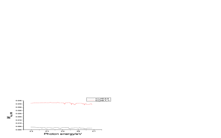
Figure 1: Transition probabilities of a hydrogen atom interacting with a circularly polarized laser of $A=5\times 10^{-6}$V$\cdot$s/m, and their dependence on the photon energy.

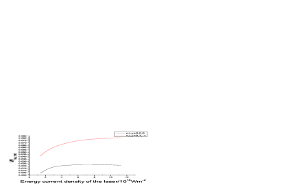
Figure 2: Transition probabilities of a hydrogen atom interacting with a circularly polarized laser of $\hbar\omega=0.296$eV, and their dependence on the laser intensity.

Fig.1 shows that the spectrum is continuous. No discrete sharp resonance peaks appear. If one fits the spectrum by

$$E_{n^{\prime}}-E_{n}=\eta\hbar\omega\ ,$$ (46)

$\eta$ may take any real number in a wide range, not necessarily be an integer. We call this kind of transition non-integer. It violates the Bohr condition. When one regards the generalized Bohr condition

$$E_{n^{\prime}}-E_{n}=N\hbar\omega$$ (47)

with integer $N$ as an expression of energy conservation, he has omitted the interaction energy between the atom and the electromagnetic field. It is permissible only when the interaction is weak and may be handled by perturbation. The non-integer transition is a typical non-perturbative effect, and the violation of Bohr condition is therefore not surprising. While fig.2 shows that the transition probability is not proportional to an integer power of the intensity. It means, the interaction between the laser and the atom cannot be reduced to interactions of individual photons with the atom separately. The interaction is between the atom and the laser as a whole. We call this character the non-linear effect. This scenery is quite different from the regularity one saw in the weak light (including weak laser) spectroscopy, therefore has to be checked by new experiments. One may observe the radiation of the atom after it has been irradiated by an intense laser. In this way, the changes of distributions of atoms among various energy levels, and therefore their transition probabilities, are measured. Although there is not any separate resonance, fig.1 still shows complex structure in the spectrum. It is interesting to find out the information exposed by this kind of structure.

V Laser photo-ionizations

The photo-ionization or the photoelectric effect is the transition of the electron from the ground state to the ionized state, when it is irradiated by light. The photo-ionization by an intense circularly polarized laser may be handled by the method proposed in z .

It is shown in z , that the energy of the ionized electron (photo-electron) is

$$E_{f0}=E_{i}-\mu\hbar\omega\ ,$$ (48)

and the transition probability per unit time is

$$P=\frac{2\pi}{\hbar}\left|H_{f0,i}^{\prime\prime}\right|^{2}\rho\ ,$$ (49)

with

$$H_{f0,i}^{\prime\prime}\equiv\int\psi_{f0}^{*}({\textit{{r}}})\hat{H}^{\prime\prime}\phi_{i}({\textit{{r}}}){\rm d}{\textit{{r}}}\ .$$ (50)

$\phi_{i}({\textit{{r}}})$ in (50) is an eigenfunction of $\hat{H}_{\rm ps}$, satisfying (32). $E_{i}$ in (48) is the corresponding eigenvalue. $\psi_{f0}({\textit{{r}}})$ is the eigenfunction of $\hat{H}_{0}^{\prime}$, with eigenvalue $E_{f0}+\mu\hbar\omega$, therefore is a projection of the Coulomb wave function onto the subspace with definite magnetic quantum number $\mu$, and describes the ionized electron.

In the weak light limit, $A\rightarrow 0$, $\phi_{i}$ approaches an eigenfunction of $\hat{H}_{0}^{\prime}$, which is also the ground state eigenfunction of $\hat{H}_{0}$ with zero magnetic quantum number; and $E_{i}$ approaches the corresponding eigenvalue. They are independent of $A$. For the hydrogen atom, they are $\psi_{100}$ and $-b$ respectively, $b$ is the binding energy of the electron in the ground state hydrogen atom. In the case of $ka_{0}<<1$, we have (42), therefore the selection rule (43) works. These limits make the energy (48) of the photoelectron be

$$E_{f0}=\hbar\omega-b\ ,$$ (51)

and the transition probability $P$ proportional to the light intensity. This example shows, in the weak light limit, the photo-ionization has the following distinct characters:

C1.There is a critical frequency for a given system.The light with frequency lower than this critical value cannot eject any electron from the system.

C2.The light with frequency higher than this critical value can ionize the system, the energy of the ejected electron increases linearly with the increasing of the frequency but is independent of the intensity of the light.

C3.The intensity of the photo-electric current is proportional to the intensity of the light.

This is exactly the experimental knowledge on photo-ionization, people had before the discovery of the laser. Based on this knowledge and guided by his idea of light quanta, one hundred years ago, Einstein e found his famous formula (51) and the idea that the light-atom interaction may be reduced to the interactions between photons and atoms. In this way, he explained the above experimental characters of photo-ionization. This was a crucial step towards the discovery of quantum mechanics. Now we see, all of these experimental characters, as well as the Einstein formula (51), together with his idea that photons interact with atoms independently, are the perturbation results of quantum mechanics in the weak light limit. What will be the scenery when the light becomes an intense laser?

If one puts $E_{1}=-b$ , and $E_{2}=E_{f0}$, the formula (51) becomes the Bohr condition $E_{2}-E_{1}=\hbar\omega$. Therefore, the Einstein formula is a predecessor of the Bohr condition. Soon after the discovery of laser, people observed MPIv and ATIa . Einstein formula was generalized to be

$$E_{f0}=N\hbar\omega-b\ ,$$ (52)

with $N$ being an positive integer. It is a special case of the generalized Bohr condition $E_{2}-E_{1}=N\hbar\omega\ ,$ and may be deduced by the higher order perturbation. (48) would be an exact expression of the photoelectron energy, if $E_{i}$ in it is solved from (32) exactly. Defining

$$\eta\equiv\frac{E_{i}+b}{\hbar\omega}-\mu\ ,$$ (53)

one may write (48) in the form

$$E_{f0}=\eta\hbar\omega-b\ .$$ (54)

It is $E_{2}-E_{1}=\eta\hbar\omega$. Here we see, $\eta$ is an integer only when $E_{i}+b-\mu\hbar\omega$ is an integer multiple of the photon energy $\hbar\omega$. This will not necessarily be the case for a non-perturbation interaction between the atom and an intense laser. It means the photo-ionization may be a non-integer quantum transition. This is a true non-perturbation effect, which cannot be handled by perturbation of any order. Using the numerical solution of (32) obtained in the last section, we find the light intensity dependence of the photoelectron energy. The numerical result is shown in fig.3.

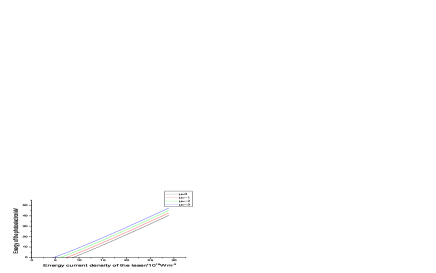
Figure 3: The energy of a photoelectron ejected from the ground state hydrogen atom by a circularly polarized laser of $\hbar\omega=2.37$eV, and its dependence on the laser intensity.

The transition probability (49) may be expressed in the form of cross section. It is the formula (14) or (15) in z . Applying it to the photo-ionization of the hydrogen atom irradiated by a circularly polarized laser, under the condition $ka_{0}<<1$, we obtain the cross section

$$\sigma=\frac{16\alpha v}{ka_{0}c}\sum_{l=|\mu|}\left|\beta_{l}(i)\right|^{2}$$ (55)

in unit of $\pi a_{0}^{2}$. Here, $v=\sqrt{2E_{f0}/m}$ is the velocity of the photoelectron, and $\beta_{l}(i)$ is an elementary but some what lengthy and tedious expression, containing integrals of the type

$$\int_{0}^{\infty}{\rm e}^{-st}t^{u-1}{\rm F}(a_{1},c_{1},t){\rm F}(a_{2},c_{2},qt){\rm d}t$$

$$=\Gamma(u)s^{-u}{\rm F}_{2}(u,a_{1},a_{2},c_{1},c_{2},s^{-1},\frac{q}{s})\ .$$ (56)

The integral has been analytically worked out. There are two confluent hypergeometric functions F on the left. One is from the radial wave function of the electron in the hydrogen atom, and another is from the Coulomb wave function of the outgoing electron. ${\rm F}_{2}$ on the right is the Appell’s hypergeometric function of the second class in two variableser . In our problem here, it degenerates into a polynomial in two variables. Therefore the calculation of $\beta_{l}(i)$ is finite, if the expansion (34) is truncated. The calculated cross section and its dependence on the laser intensity is shown in fig.4.

Figure 4: Cross section of the photo-ionization of a ground state hydrogen atom irradiated by a circularly polarized laser of $\hbar\omega=2.37$eV, and its dependence on laser intensity.

We see from fig.3, the energy of the photo-electron increases with the increasing of the light intensity. The critical frequency is not absolute. Even though the frequency of the incident light is lower than the critical frequency, the electron may still be ejected, if the light is intense enough. The characters C2 and C1, together with the formula (51), are not true for intense laser photo-ionization. Furthermore, the formula (52) is not true either, if the incident laser is very intense. In this case, it has to be substituted by (54), with possibly non-integer $\eta$. The transition in photo-ionization becomes non-integer. However, one may still see an apparent quantum character in fig.3. That is, the energy difference between photo-electrons with different magnetic quantum number $\mu$ is an integer multiple of the quantum energy $\hbar\omega$, as people observed in ATI. From fig.4 we see, the cross sections depend on the light intensity nonlinearly. It means that the character C3 is not true for laser photo-ionization. The interaction between light and atoms cannot be reduced to the independent interactions between photons and atoms. Atoms interact with the laser as a whole. This is the non-linear effect.

VI Conclusion

We see, a laser may not only induce MPI, but also cause non-integer transitions, if it is strong enough. The later can only be handled by non-perturbation method, and therefore is a true non-perturbative effect. The non-linear effect in atom-laser interaction is also noticeable. Some quantitative details are exposed in above sections. The correctness of these predictions have to be finally checked by experiments. It now calls for appropriate experiments.

Quantum electrodynamics is the best theory nowadays. It has been checked in details around the vacuum state. However, its correctness in presence of a intense electromagnetic wave still has to be checked. We need reliable method to explore its solutions and compare the results with experiments. The above method simplifies the work considerably when the laser is circularly polarized. It may be used for more general cases, to consider, for examples, the spin, the relativity, as well as other atoms and molecules.

The work is supported by the National Nature Science Foundation of China with grant number 10305001.

References

- (1) G.S. Voronov and N.B. Delone ,Zh. Eksp. Teor. Fiz. 50,(1966)78 [Sov. Phys. JETP 23 (1966) 54]
- (2) P. Agostini, F. Fabre, G. Mainfray, G. Petite and N.K. Rahman, Phys.Rev.Lett. 42, (1979) 1127
- (3) Y. Gontier, M. Poirer and M. Trahin, J. Phys. B 13 (1980) 1381
- (4) P.H.Bucksbaum, D.W.Schumacher, M.Bashkansky, Phys. Rev. Lett. 61(1988) 1182
- (5) P.L.Kapitza and P.A.M.Dirac, Proc. Camb. Phil. Soc. 29 (1933) 297
- (6) D.-S. Guo, G.W.F.Drake, Phys. Rev. A 45 (1992) 6622
- (7) D.-S. Guo, T. Åberg, and B. Crasemann, Phys. Rev. A40 (1989) 4997
- (8) L. V. Keldysh, Zh. Eksp. Teor. Fiz. 50 (1966) 18 [Sov. Phys. JETP 20 (1965) 1307]
- (9) F. H. M. Faisal, J. Phys. B6 (1973) L89
- (10) H. R. Reiss, Phus. Rev. A22 (1980) 1786
- (11) H.Batelaan, Contemporary Physics 41 (2000) 369
- (12) D.L.Freimund, K.Aflatooni, H.Batelaan, Nature 413 (2001) 142
- (13) C.-L. Xiong and Q.-R. Zhang , Commun. Theor. Phys. 42 (2004)891
- (14) K. J. LaGattuta, Phys. Rev. A 41 (1990) 5110
- (15) Y. I. Salamin, Phys. Rev. A 56 (1997) 4910
- (16) Qi-Ren Zhang , Phys. Lett. A 216 (1996) 125
- (17) Deng Zhang and Qi-Ren Zhang, Comm. Theor. Phys. 36 (2001) 685
- (18) J.H. Wilkinson The Algebraic Eigenvalue Problem, Clarendon Press, Oxford, 1965
- (19) A. Einstein Ann. Phys. (Leipzig) 17 (1905) 132
- (20) A. Erdlyi Higher Transcendental Functions I, McGraw Hill, New York, 1953