Entanglement quantification through local observable correlations

Abstract

We present a significantly improved scheme of entanglement detection inspired by local uncertainty relations for a system consisting of two qubits. Developing the underlying idea of local uncertainty relations, namely correlations, we demonstrate that it’s possible to define a measure which is invariant under local unitary transformations and which is based only on local measurements. It is quite simple to implement experimentally and it allows entanglement quantification in a certain range for mixed states and exactly for pure states, without first obtaining full knowledge (e.g. through tomography) of the state.

I Introduction

Entanglement is one of the key resources in quantum mechanics and in particular in quantum communication and quantum information applications. Its appearance and behavior was discovered and discussed a long time ago EPR ; SR , but it was only since the 1980s that applications of entanglement, like quantum teleportation Ben , quantum cryptography BB84 ; Eke and quantum algorithms Deu ; Sho ; Gro , were developed and became the focus for intense research.

An important question which is not answered in full generality yet is: Assuming a given state, how much “profit” (in terms of entanglement) is inherently hidden in that state that could be used to perform some of the tasks mentioned above? A state with higher entanglement should allow us to perform a task in some sense better than a state with lower entanglement. Therefore a lot of effort has been spent during the last two decades to investigate entanglement further, and in particular, to quantify it HHH ; Hor , so that states can be quantitatively ranked. For the case of two qubits, substantial progress has been achieved and entanglement of formation and concurrence are widely accepted as well behaved and operationally meaningful measures for entanglement Woot2 . However, for higher-dimensional cases and multipartite states the situation gets more complicated and, despite some progress, the search for good measures is still going on RB ; AF ; EG .

Even if good measures exist for the case of two qubits, they require, in general, full knowledge of the density matrix for a given state to be determined. This is achieved by full state tomography Du , a cumbersome and time-consuming experimental measurement process. A way to avoid these inconveniences is to use so-called entanglement witnesses LK ; LK2 ; GL , which can detect specific entanglement, but, on the other hand, are not able to quantify it. An alternative to entanglement witnesses are local uncertainty relations (LUR) HT . They are typically easy to implement experimentally, but unfortunately no known LUR can detect all entangled two-qubit states, and in general they do not give quantitative measure of entanglement for the states they do detect. Assuming that one has an unknown state, it is therefore desirable to quantify its entanglement as well as possible, with the lowest possible experimental effort.

In this paper we will extend the idea of local uncertainty relations for two qubits and thereby overcome most of its drawbacks, but keeping it’s advantages. We will derive a measure that is invariant under local unitary transformations, and which quantifies entanglement for all pure states and in some range for mixed states. An advantage is that the measure only requires local measurements (in contrast to BH , for example), facilitating the experimental effort. A mathematically similar approach as ours has been taken by de Vicente Vicente , who use the Bloch-vector representation of bipartite states and the Ky Fan norm to write an inequality that can only be broken by nonseparable states. However, Vicente does not address how his entanglement criteria can be experimentally implemented.

Compared to state tomography our measure will require the same number of measurement-settings for the case of two qubits (9 settings), but we conjecture significantly less measurement-setups in higher-dimensional systems. On the other hand one can always calculate the concurrence after a state tomography, since one has full knowledge of the state. The simplest LUR requires only 2 measurement-settings KH but LURs are (except some special cases) not able to quantify entanglement.

In the next section we will motivate the measure starting from local uncertainty relations and then discuss it’s properties. After that we will investigate the case of pure states in section III and the case of mixed state in section IV, before summarizing the results and discuss still open questions in section V.

II Definition and implementation

Before giving the definition of the new measure, we will motivate it by giving a short review of entanglement detection through local uncertainty relations. Even though the theory of local uncertainty relations has been extended to multipartite systems by Gühne OG , we will only cover bipartite systems here. Having two systems $A$ and $B$, one can choose sets of observables $\{\hat{A}_{i}\}$ and $\{\hat{B}_{i}\}$, acting solely on the corresponding system. In each set of observables it is assumed that the observables have no joint eigenvector. The local variances are then given by $\delta^{2}\hat{A}_{i}\equiv\left\langle\hat{A}_{i}^{2}\right\rangle-\left\langle\hat{A}_{i}\right\rangle^{2}$, and similar for $\delta^{2}\hat{B}_{i}$. These variances are nonnegative, and for the variance $\delta^{2}\hat{A}_{i}$ to be zero the system has to be in an eigenstate of $\hat{A}_{i}$. Because the operators $\{\hat{A}_{i}\}$ have no joint eigenstates the variance $\delta^{2}\hat{A}_{j}$ for this state must be positive for all $j\neq i$. Therefore, there exist a state (or a class of states) that have an associated non-trivial value $U_{A}>0$ which is the greatest lower limit of the sum of the variances. From this follows that for any state the following inequality holds:

$$\sum\limits_{i}\delta^{2}\hat{A}_{i}\geq U_{A}.$$ (1)

The same thing holds for the observables of system $B$ and we will define $U_{B}$ in the same way, so that

$$\sum\limits_{i}\delta^{2}\hat{B}_{i}\geq U_{B}.$$ (2)

The operators $\hat{A}_{i}+\hat{B}_{i}$ can be defined to measure properties of the common system. One can show that the local uncertainty relation

$$\sum\limits_{i}\delta^{2}\left(\hat{A}_{i}+\hat{B}_{i}\right)\geq U_{A}+U_{B}$$ (3)

then holds for all statistical mixtures of product states. A proof for (3) for this class of states is given in HT .

Expanding the left hand side of Eq. (3) gives

$$\sum\limits_{i}\delta^{2}\left(\hat{A}_{i}+\hat{B}_{i}\right) = \sum\limits_{i}\delta^{2}\hat{A}_{i}+\sum\limits_{i}\delta^{2}\hat{B}_{i}$$ (4)

$$+2\sum\limits_{i}C\left(\hat{A}_{i},\hat{B}_{i}\right),$$

where the covariance term is defined as

$$C\left(\hat{A}_{i},\hat{B}_{i}\right)=\left\langle\hat{A}_{i}\hat{B}_{i}\right\rangle-\left\langle\hat{A}_{i}\right\rangle\left\langle\hat{B}_{i}\right\rangle.$$ (5)

To reveal entanglement by not fulfilling inequality (3), one can immediately see, that at least one of the covariance terms has to be less than zero for such an entangled state. Any single covariance term is bounded by

$$-\left(\delta^{2}\hat{A}_{i}+\delta^{2}\hat{B}_{i}\right)\leq 2C\left(\hat{A}_{i},\hat{B}_{i}\right)\leq\delta^{2}\hat{A}_{i}+\delta^{2}\hat{B}_{i}.$$ (6)

Since both bounds can be reached with both mixed separable and pure entangled states for any particular choice of a pair of observables $\hat{A}_{i}$ and $\hat{B}_{i}$, one has to look at several covariances to detect entanglement. To give an example, one can consider a two-level system, e.g., the polarization states of spatially separated photon pairs. A possible LUR in this case is

$$L_{3} = \delta^{2}\left(\hat{\sigma}^{A}+\hat{\sigma}^{B}\right)_{0/90}+\delta^{2}\left(\hat{\sigma}^{A}+\hat{\sigma}^{B}\right)_{45/135}$$ (7)

$$+\delta^{2}\left(\hat{\sigma}^{A}+\hat{\sigma}^{B}\right)_{R/L}\geq 4,$$

where the subscript 0/90 denotes measurements of horizontal and vertical linear polarization. Assume that the measurement eigenvalues for $\hat{\sigma}^{A}$ and $\hat{\sigma}^{B}$ are $\pm 1$. This means that the possible measurement outcomes for $\hat{\sigma}^{A}+\hat{\sigma}^{B}$ are -2, 0, and 2. The subscript 45/135 denotes similar measurements in a basis rotated by 45 degrees and R/L denotes measurements of left- and right-handed polarized photons. The relation (7) was investigated by Ali Khan and Howell in KH and $L_{3}\geq 4$ is fulfilled by all mixtures of separable states, but may be violated for entangled states, the minimum of $L_{3}$ being zero in this latter case. The lower bound $L_{3}=0$ is attained by the singlet state $(\left\langle\uparrow,\downarrow\right|-\left\langle\downarrow,\uparrow\right|)/\sqrt{2}$ because this state has perfectly anticorrelated polarization if photon $A$ and $B$ are measured in any same basis. Therefore $L_{3}$ can detect entanglement. Note, however, that $L_{3}$ assumes a shared spatial reference frame, because if $A$ and $B$ are measured with the respective horizontal and vertical axes unaligned, $L_{3}$ will no longer be zero for the singlet state. In addition, only a small fraction of the set of entangled qubit states is detected by $L_{3}$ and a local unitary transformation of a given entangled state is sufficient to make a violated LUR fulfilled, or vice versa, although the entanglement remains invariant per definition. As an example, a local basis-state flip on either $A$ and $B$ (which is equivalent to an interchange of the vertical and the horizontal axis) results in the state $(\left\langle\uparrow,\uparrow\right|-\left\langle\downarrow,\downarrow\right|)/\sqrt{2}$ for which $L_{3}$ takes its maximum value eight, well over the threshold for entanglement detection, which is four. This example demonstrates the necessity of a shared spatial reference frame. If we, on the other hand, were using a measure which is invariant under local unitary transformations we would not have to align our measurement setups, since every local rotation can be described by a local unitary transformation. Especially if the measurement devices are located far apart this can lower the experimental effort significantly.

An attempt to rectify some of the problems with LURs was done in SB , where an improved way of using local uncertainty relations, so called modified local uncertainty relations (MLUR), was proposed. These MLUR could detect more states than LUR, but the main drawbacks of local uncertainty relations, namely invariance under local unitary transformations, remained. An advantage of LURs, compared to state tomography or entanglement witnesses, is the relatively small experimental effort which is needed to implement them experimentally. Therefore we propose in this paper a new measure inspired by local uncertainty relations, which keeps the advantages of LUR like low experimental effort, but gets rid of some of the disadvantages of LUR, for example being not invariant under local unitary transformations, not detecting all entangled pure states or not quantifying entanglement.

One realizes that the information of entanglement is somehow coded in the covariances defined by Eq. (5), since only they are responsible for violating a LUR. We propose therefore for the case of two qubits to use the sum of all possible covariances between two local sets of mutually unbiased bases, one for each qubit,

$$G=\sum\limits_{i,j=1}^{3}C^{2}\left(\hat{\sigma}_{i}^{A},\hat{\sigma}_{j}^{B}\right),$$ (8)

as a measure of entanglement. Here, $\hat{\sigma}_{i}^{A}$ denotes the $i$:th Pauli matrix (operator) for system $A$, and similar for $B$. The Pauli matrices are

$$\hat{\sigma}_{1}=\left(\begin{array}[c]{cc}0&1\\ 1&0\end{array}\right),\hat{\sigma}_{2}=\left(\begin{array}[c]{cc}0&-i\\ i&0\end{array}\right),\hat{\sigma}_{3}=\left(\begin{array}[c]{cc}1&0\\ 0&-1\end{array}\right),$$ (9)

whose eigenvalues are $\pm 1$. The Pauli matrices are traceless: $\mathrm{Tr}\left(\hat{\sigma}_{i}\right)=0$ (for $i=1,2,3$). In the following we will denote the unity matrix as $\hat{\sigma}_{0}$:

$$\hat{\sigma}_{0}=\left(\begin{array}[c]{cc}1&0\\ 0&1\end{array}\right).$$ (10)

These four matrices have the property $\mathrm{Tr}\left(\hat{\sigma}_{i}\hat{\sigma}_{j}\right)=2\delta_{ij}$ for $i,j=0,\ldots,4$. The measure of Eq. (8) is easy to implement. Since

$$C\left(\hat{\sigma}_{i}^{A},\hat{\sigma}_{j}^{B}\right)=\left<\hat{\sigma}_{i}^{A}\otimes\hat{\sigma}_{j}^{B}\right>-\left<\hat{\sigma}_{i}^{A}\otimes\hat{\openone}^{B}\right>\left<\hat{\openone}^{A}\otimes\hat{\sigma}_{j}^{B}\right>,$$ (11)

one has only to count singles rates and coincidences. The measurements can be performed locally on each system and a total of nine measurement-settings are sufficient ($\left<\hat{\sigma}_{i}\otimes\hat{\openone}\right>$ and $\left<\hat{\openone}\otimes\hat{\sigma}_{j}\right>$ can be calculated from the other measurements) to get all the results. Here, we would like to point out that $G$ is invariant under any local unitary transformations. That is, $G\left(\hat{\rho}\right)=G\left(\hat{U}\hat{\rho}\hat{U}^{\dagger}\right)$ with $\hat{U}=\hat{U}_{A}\otimes\hat{U}_{B}$ where $\hat{U}_{A}$ ($\hat{U}_{B}$) operates only on subsystem A (B). ($G$ is also invariant under partial transposition.) The invariance is a direct consequence of the fact that our measure $G$ can be rewritten as

$$G=4\mathrm{Tr}\left\{\left(\hat{\rho}-\hat{\rho}_{A}\otimes\hat{\rho}_{B}\right)^{2}\right\},$$ (12)

that is, in terms of the Hilbert-Schmidt norm measure of distance, where $\hat{\rho}_{A}$ denotes the density matrix of system $A$ after tracing over system $B$ and similar for $\hat{\rho}_{B}$ Hall . Since any unitary transformation can be seen as a rotation or mirroring of the basis vectors of a Hilbert-space and a norm is invariant under rotation or mirroring the basis, it follows that $G$ is invariant under any local unitary transformation. To see the equivalence between Eq. (8) and Eq. (12) one can expand the density matrix $\hat{\rho}_{A}$ as

$$\hat{\rho}_{A}=\frac{1}{2}\sum\limits_{n=0}^{3}\mathrm{Tr}\left(\hat{\openone}\otimes\hat{\sigma}_{n}\hat{\rho}\right)\hat{\sigma}_{n}$$ (13)

and similar for $\hat{\rho}_{B}$. $\hat{\rho}$ can also be expanded in the basis defined by the operators $\hat{\sigma}_{i}$ as

$$\hat{\rho}=\frac{1}{4}\sum\limits_{n=0}^{3}\sum\limits_{m=0}^{3}\mathrm{Tr}\left(\hat{\sigma}^{A}_{m}\otimes\hat{\sigma}^{B}_{n}\hat{\rho}\right)\hat{\sigma}^{A}_{m}\otimes\hat{\sigma}^{B}_{n}.$$ (14)

Inserting the expansion (13) and its $\hat{\rho}_{B}$ counterpart, and (14) into (12), and using the Pauli matrix relations written just under (9) and (10), it is not difficult to rewrite the ensuing equation in the form (8).

Note that, because of the local unitary invariance is it not necessary to use the Pauli matrices in the definition of our proposed measure in Eq. (8). Every local unitary transformation of this mutually unbiased basis (MUB) KW works equally well. The invariance under local unitary transformations also means that a shared spatial reference frame is no longer needed, because a local rotation (a unitary transformation) will leave the measure invariant. However, since it is sufficient to use the Pauli matrices and since they are convenient from an experimental and mathematical viewpoint, we will continue to use them in this paper.

For pure states $G$ is just a bijective function of the well-established concurrence, whereas for mixed states $G$ relates a state to a certain range of concurrence. The proof of these statements are given next.

III Pure states

We will relate our measure to the well known concurrence in the case of pure states. For the proof we will expand an ordinary pure two-qubit state into the eigenvectors $\left|00\right\rangle$, $\left|01\right\rangle$, $\left|10\right\rangle$ and $\left|11\right\rangle$ of the $\hat{\sigma}_{3}^{A}\otimes\hat{\sigma}_{3}^{B}$ operator, that is

$$\left|\psi\right\rangle = a_{00}\left|00\right\rangle+a_{01}\left|01\right\rangle+a_{10}\left|10\right\rangle+a_{11}\left|11\right\rangle$$ (15)

$$= \sum\limits_{k,l=0}^{1}\alpha_{kl}\left|k\right\rangle^{A}\otimes\left|l\right\rangle^{B}.$$

The adjoint state can be written in a similar way and, dropping the sign for the tensor product, we can expand

$$G = \sum\limits_{i,j=1}^{3}\left(\left<\hat{\sigma}_{i}^{A}\hat{\sigma}_{j}^{B}\right>^{2}-2\left<\hat{\sigma}_{i}^{A}\hat{\sigma}_{j}^{B}\right>\left<\hat{\sigma}_{i}^{A}\right>\left<\hat{\sigma}_{j}^{B}\right>\right.$$ (16)

$$+\left.\left<\hat{\sigma}_{i}^{A}\right>^{2}\left<\hat{\sigma}_{j}^{B}\right>^{2}\right)$$

in a sum of products of the expansion coefficients $\alpha_{kl}$.

Recall now the results of Linden and Popescu LP , where they derive the invariants of systems of different dimensions under local unitary transformations. For the case of two qubits they show that there are only two invariants:

$$I_{1} = \sum\limits_{k,l=0}^{1}\alpha_{kl}\alpha_{kl}^{\ast}$$ (17)

$$I_{2} = \sum\limits_{k,l,m,n=0}^{1}\alpha_{km}\alpha_{kn}^{\ast}\alpha_{ln}\alpha_{lm}^{\ast}.$$ (18)

Evaluating the expansion of Eq. (16) performing considerable trivial, but tedious, algebra (i.e. evaluating all the terms $\left\langle\cdot\right|\hat{\sigma}\left|\cdot\right\rangle$ and making the summation), the result is

$$G=\left(I_{\alpha}^{2}+8I_{\beta}\right)-2I_{\alpha}\left(I_{\alpha}^{2}-4I_{\beta}\right)+\left(I_{\alpha}^{2}-4I_{\beta}\right)^{2},$$ (19)

where the first term in Eq. (19) corresponds to the first term in the Eq. (16) and so on. The summation over $i$ and $j$ is already included in each term. $I_{\alpha}$ and $I_{\beta}$ stand for

$$I_{\alpha} = \left|\alpha_{00}\right|^{2}+\left|\alpha_{01}\right|^{2}+\left|\alpha_{10}\right|^{2}+\left|\alpha_{11}\right|^{2}$$ (20)

$$I_{\beta} = \left(\alpha_{01}\alpha_{10}-\alpha_{00}\alpha_{11}\right)\left(\alpha_{01}^{\ast}\alpha_{10}^{\ast}-\alpha_{00}^{\ast}\alpha_{11}^{\ast}\right)$$ (21)

$$= \left|\alpha_{00}\alpha_{11}-\alpha_{01}\alpha_{10}\right|^{2}.$$ (22)

One sees immediately that $I_{\alpha}=I_{1}$. If one looks at Eq. (19) in further detail one sees that $I_{\alpha}$ is not just a constant under unitary transformations, it is simply the state normalization constant and therefore $I_{\alpha}=1$ for all states. One can, after some algebra, also show that $I_{\beta}=(I_{1}^{2}-I_{2})/2$. Therefore $I_{\beta}$ is also an invariant. This simplifies equation (19) to

$$G=8I_{\beta}+16I_{\beta}^{2}=4I_{\beta}\left(2+4I_{\beta}\right).$$ (23)

Knowing that $4I_{\beta}={\cal C}^{2}$ AF , where ${\cal C}$ denotes the well-known concurrence Woot2 for pure states, we finally get

$$G={\cal C}^{2}\left(2+{\cal C}^{2}\right).$$ (24)

The concurrence is related to entanglement of formation and having therefore a pure state, one can directly quantify its entanglement by measuring $G$. For a pure state $G>0$ implies that the state is entangled. This is an intuitive result because a separable, pure state cannot display any covariance between local measurements.

IV Mixed states

The relation between $G$ and the concurrence that held for the pure states in Eq. (24) is no longer valid for mixed states. Instead, $G$ can, in general, take any value in the shaded region plotted in Fig. 1. That is, $0\leq G\leq 3$ or, if we write it in relation to the concurrence, one has

$${\cal C}^{2}\left(2+{\cal C}^{2}\right)\leq G\leq 1+2{\cal C}^{2}.$$ (25)

The lower bound of this inequality is given by Eq. (24), that is, any pure state has the lowest possible values of $G$ for a given amount of entanglement. The reason for that is that correlations for pure states can only be given by entanglement. (Note that the converse is not true. That is, there are mixed states that also saturate the lower bound of $G$.)

To find the upper bound of Eq. (25) we look at the density matrix

$$\hat{\rho}_{u}=\left(\begin{array}[c]{cccc}1/2&0&0&e^{i\theta}\gamma\\ 0&0&0&0\\ 0&0&0&0\\ e^{-i\theta}\gamma&0&0&1/2\end{array}\right)$$ (26)

with $0\leq\gamma\leq 1/2$ and $\theta$ an arbitrary real number. The class of states defined by this density matrix interpolates between maximally classically correlated states with no entanglement ($G=1$, ${\cal C}=0$ when $\gamma=0$) and maximally entangled (pure) states which have the highest correlations of any states ($G=3$, ${\cal C}=1$ when $\gamma=1/2$). It is reasonable to believe that this class of states has the highest value of $G$ for any given amount of entanglement. Using the definition of $G$ in Eq. (8) one finds that for these states $G(\hat{\rho}_{u})=1+8\gamma^{2}$. Calculating the concurrence gives ${\cal C}(\hat{\rho}_{u})=2\gamma$ and therefore we have $G(\hat{\rho}_{u})=1+2{\cal C}^{2}$. A simulation with many thousands of arbitrary states shows that, indeed, no state is outside the range given by (25). Hence, a value of $G>1$ guarantees that the system is entangled, since $G$ of separable states (having zero concurrence) cannot exceed unity.

Unfortunately, we don’t have any strict algebraical proof for the limits of $G$ at the moment although we firmly believe, and can see clear arguments why the limits are both sufficient and necessary. The problem is that it is not known how to parameterize the entire class of states with a given concurrence, let alone to find the maximum G of such a multiparameter class of states.

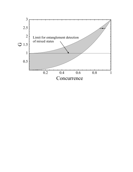
Figure 1: Bounds for $G$ when plotted over the concurrence. See text for more details.

In general, $G$ is an “entanglement witness” for mixed states, since it can detect entanglement for a class of states. But if one has a state with a high concurrence, $G$ can give more information. An example is given in Fig. 1. Imagine one measures a value of $G=2.5$. In that case, the state has to have a concurrence somewhere in the range of the upper horizontal line in Fig. 1, that is

$$0.87\leq{\cal C}\leq 0.93.$$ (27)

This is quite a narrow range. Hence, even if one is not able to determine the concurrence exactly, $G$ is still able to limit a state to a certain range of the concurrence. Assigning a value of ${\cal C}=0.9$ in the case above would, for example, only give a maximum error of $\pm 4\%$ for the concurrence. $G$ is therefore giving more information about a state than an entanglement witness ordinarily does.

An interesting question is, whether $G$ can somehow be “compensated” by the amount of mixedness, so that $G$ and ${\cal C}$ become a bijective map also for mixed states. We have made some simulations with arbitrary density matrices and plotted $G$ as a function of the concurrence and of the degree of purity, defined by $Tr\left(\hat{\rho}^{2}\right)$ (see MJ ). The result can be seen in Fig. 2. If one fixes the concurrence to a certain value and just looks at $G$ depending on the purity, it turns out that these simulation results cover an area and not only a line, showing that it is impossible, to write the measure as $G=G\left({\cal C}\left(\hat{\rho}\right),Tr\left(\hat{\rho}^{2}\right)\right)$ and thereby “compensating” $G$ by the purity. However, one might use other definitions than $Tr\left(\hat{\rho}^{2}\right)$ for the mixedness to fulfill this. This is still an open question.

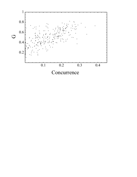
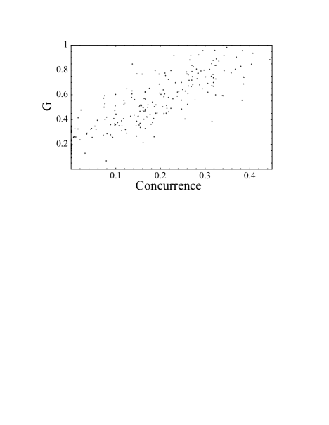
Figure 2: Simulation results of measuring $G$ for some mixed states. The upper figure is for states with a purity of $\mathrm{Tr}\left(\hat{\rho}^{2}\right)=0.46\pm 0.005$ and the lower figure is for states with $\mathrm{Tr}\left(\hat{\rho}^{2}\right)=0.5\pm 0.005$.

V Summary and discussion

Inspired by local uncertainty relations we have suggested a measure of entanglement for two qubits, which can quantify entanglement for pure states and can give bounds on the entanglement of mixed states. This measure is invariant under local unitary transformations and requires only local measurements to be implemented. It might even be possible to get an exact quantification for mixed states.

Further work will be focused on which properties a generalization of our proposal would have for higher dimensional systems. In this connection we can refer to Wootters Woot , who showed that one can determine all properties of a state by measuring all combinations of local MUB eigenstate projections and the identity matrix. We therefore conjecture that a generalization of our proposed measure for higher-dimensional systems would keep the properties like invariance under local unitary transformations and can be useful to detect and quantify entanglement.

In that context the number of measurement-settings for our measure would scale substantially lower as a function of the dimensions as the number of measurement setups would scale for state tomography. For multi-partite systems a similar method may still work, but in this case the added complication that different kinds of entanglement exist makes the problem both a quantitative and a qualitative one.

VI Acknowledgements

The authors want to thank Drs. Michael Hall and Otfried Gühne for fruitful correspondence. This work was supported by the Swedish Research Council (VR), the Swedish Foundation for Strategic Research (SSF), and the European Community through grant Qubit Applications #015848.

References

- (1) A. Einstein, B. Podolsky, and N. Rosen, Phys. Rev. 47, 777 (1935).
- (2) E. Schrödinger, Naturwissenschaften 23, 807, 823, 844 (1935).
- (3) C. H. Bennett, G. Brassard, C. Crépeau, R. Jozsa, A. Peres, and W. K. Wootters, Phys. Rev. Lett. 70, 1895 (1993).
- (4) C. H. Bennett and G. Brassard in Proceedings of IEEE International Conference on Computers, Systems and Signal Processing, Bangalore, India, 1984 (IEEE, New York, 1984), p. 175.
- (5) A. K. Ekert, Phys. Rev. Lett. 67, 661 (1991).
- (6) D. Deutsch, Proc. R. Soc. A 400, 97 (1985).
- (7) P. W. Shor, SIAM J. Comp. 26, 1484 (1997).
- (8) L. K. Grover, Phys. Rev. Lett. 79, 325 (1997).
- (9) G. Alber, T. Beth, M. Horodecki, P. Horodecki, R. Horodecki, M. Rötteler, H. Weinfurter, R. Werner, A. Zeilinger, Quantum Information: An Introduction to Theoretical Concepts and Experiments, (Springer, Berlin 2001).
- (10) M. Horodecki, Quantum Information and Communication 1, 3 (2001).
- (11) W. K. Wootters, Phys. Rev. Lett. 80, 2245 (1998).
- (12) P. Rungta, V. Bužek, C. M. Caves, M. Hillery, and G. J. Milburn, Phys. Rev. A 64, 042315 (2001).
- (13) S. Albeverio and S.-M. Fei, J. Opt. B: Quantum Semiclass. Opt. 3, 223 (2001).
- (14) J. Eisert and D. Gross, quant-ph/0505149.
- (15) T. Durt, quant-ph/0604117.
- (16) M. Lewenstein, B. Kraus, J. I. Cirac, and P. Horodecki, Phys. Rev. A 62, 052310 (2000).
- (17) M. Lewenstein, B. Kraus, P. Horodecki, and J. I. Cirac, Phys. Rev. A 63, 044304 (2001).
- (18) O. Gühne and N. Lütkenhaus, Phys. Rev. Lett. 96, 170502 (2006).
- (19) H. F. Hofmann and S. Takeuchi, Phys. Rev. A 68, 032103 (2003).
- (20) S. Bose and D. Home, Phys. Rev. Lett. 88, 050401 (2002).
- (21) J. I. de Vicente, quant-ph/0607195.
- (22) I. Ali Khan and J. C. Howell, Phys. Rev. A 70, 062320 (2004), ibid 73, 049905 (2006).
- (23) O. Gühne, Phys. Rev. Lett. 92, 117903 (2004).
- (24) S. Samuelsson and G. Björk, Phys. Rev. A 73, 012319 (2006).
- (25) We want to thank Dr. Michael Hall for pointing out this relation, and Ref. [21], to us.
- (26) O. Krueger and R. F. Werner, quant-ph/0504166, p. 43
- (27) W. J. Munro, D. F. V. James, A. G. White, and P. G. Kwiat, Phys. Rev. A 64, 030302(R) (2001).
- (28) N. Linden and S. Popescu, Fortschr. Phys. 46, 567 (1998).
- (29) W. K. Wootters in Complexity, Entropy, and the Physics of Information, SFI Studies in the Sciences of Complexity, edited by E. H. Zurek (Addison-Wesley, 1990), Vol. VIII, p. 39.