Exact Casimir interaction between eccentric cylinders

Abstract

The Casimir force is the ultimate background in ongoing searches of extra-gravitational forces in the micrometer range. Eccentric cylinders offer favorable experimental conditions for such measurements as spurious gravitational and electrostatic effects can be minimized. Here we report on the evaluation of the exact Casimir interaction between perfectly conducting eccentric cylinders using a mode summation technique, and study different limiting cases of relevance for Casimir force measurements, with potential implications for the understanding of mechanical properties of nanotubes.

As the size of physical systems is scaled down into the micrometer and submicrometer scales, macroscopic quantum effects become increasingly important. Forces attributable to the reshaping of quantum vacuum fluctuations under changes in geometrical boundary conditions, predicted almost sixty years ago by Casimir Casimir1948 , have been measured in recent years with increasing accuracy Lamoreaux1997 ; Mohideen1998 ; Ederth2000 ; Chan2001 ; Bressi2002 ; Decca2003 . The fact that the magnitude and sign of the Casimir force depend both on the geometry and material structure of the boundaries paves the way to several opportunities and challenges for engineering mechanical structures above the nanoscale Chan2001prl .

The Casimir interaction for perfect metals has been exactly evaluated only for a limited number of geometries, starting from the original parallel plate configuration Casimir1948 . Until recently, for all non-planar geometries the Casimir force has been estimated using the so-called proximity-force approximation (PFA) Derjaguin1 , semiclassical Schaden00 ; Mazzitelli2003 and optical approximations Jaffe2004 , and numerical path-integral methods Gies2003 . This has originated a debate on the assessment of the accuracy of the measurements, a crucial issue to establish reliable limits on extra-gravitational forces in the micrometer range. In the last months large violations of PFA for corrugated plates have been reported Rodrigues2006 , and the exact Casimir interaction between a sphere in front of a plane and a cylinder in front of a plane has been computed Gies2006 ; Wirzba2006 ; Emig2006 . As first discussed in Dalvit2004 , the cylinder-plane configuration is intermediate between the plane-plane and sphere-plane geometries, offering easier parallelization than the former one, and a larger absolute signal than the latter one due to its extensivity in the length of the cylinder. A related experimental attempt aiming to measure temperature corrections to the Casimir force is under development BrownHayes2005 .

In this Rapid Communication we present the exact evaluation of the Casimir interaction for another geometry of experimental relevance consisting of two perfectly conducting eccentric cylinders. Although parallelism is as difficult as for the plane-plane geometry, this geometry offers several experimental advantages. First, Gauss law dictates that the expected gravitational force is zero for any location of the inner cylinder, which allows for a null experiment when looking for intrinsically short-range extra-gravitational forces. Second, the fact that the concentric configuration is an unstable equilibrium position Dalvit2004 opens the possibility of measuring the derivative of the force using closed-loop experiments. Finally, residual electrostatic charges on the surfaces can be exploited to maximize the parallelism between the cylinders looking at the minimum value of the resulting Coulomb force.

Before embarking on the exact calculation of the Casimir energy for this geometry, let us recall the result of the PFA. This is a simple, though uncontrolled way, of treating non-planar configurations, and is valid for surfaces whose separation is much smaller than typical local curvatures. For two very long eccentric cylinders of radii $a<b$, length $L$, and eccentricity $\epsilon$ (see Fig. 1), the PFA approximation for the non-concentric Casimir energy reads $E_{\rm PFA}=-\pi^{3}\hbar cL\epsilon^{2}/120a^{4}(\alpha-1)^{5}$, valid when $\alpha\equiv b/a\rightarrow 1$ and for small eccentricity $\delta\equiv\epsilon/a\ll 1$. In the limit of large eccentricity ($\epsilon\approx b-a$) PFA predicts a behavior similar to that of a cylinder in front of a plane Dalvit2004 . The geometrical dimensionless parameters $\alpha$ and $\delta$ fully characterize the eccentric cylinders configuration.

Figure 1: Geometrical configuration studied in this paper. Two perfectly conducting eccentric cylinders of radii $a<b$, length $L$, and eccentricity $\epsilon$ interact via the Casimir force. The equilibrium position at $\epsilon=0$ is unstable - any small perturbation will make the cylinders snap into each other.

In order to go beyond the PFA result, we start by expressing the Casimir energy as $E=(\hbar/2)\sum_{p}(\omega_{p}-\tilde{\omega}_{p})$, where $\omega_{p}$ are the eigenfrequencies of the electromagnetic field satisfying perfect conductor boundary conditions on the cylindrical surfaces, and $\tilde{\omega}_{p}$ are the corresponding ones to the reference vacuum (cylinders at infinite separation). In cylindrical coordinates, the eigenmodes are $h_{n,k_{z}}=R_{n}(r,\theta)\exp[-i(\omega_{n,k_{z}}t-k_{z}z)]$, where $\omega_{p}=\omega_{n,k_{z}}=\sqrt{k_{z}^{2}+\lambda_{n}^{2}}$, and $R_{n}$ ($\lambda_{n}$) are the eigenfunctions (eigenvalues) of the 2D Helmholtz equation. Using the argument theorem the sum over eigenmodes can be written as an integral over the complex plane, with an exponential cutoff for regularization. In order to determine the part of the energy that depends on the separation between the two cylinders it is convenient to subtract the self-energies of the two isolated cylinders, $E_{12}(a,b,\epsilon)=E-E_{1}(a)-E_{1}(b)$. Then the divergencies in $E$ are cancelled out by those ones in $E_{1}(a)$ and $E_{1}(b)$, and the final result for the interaction energy is

$$E_{12}(a,b,\epsilon)=\frac{\hbar cL}{4\pi}\int_{0}^{\infty}dy\;y\;\log M(iy).$$ (1)

Here $M=(F/F_{\infty})/[(F_{1}(\infty)/F_{1}(a))\;(F_{1}(\infty)/F_{1}(b))]$. The function $F$ is analytic and it vanishes at all the eigenvalues $\lambda_{n}$ ($F_{\infty}$, at $\tilde{\lambda}_{n}$), and, similarly, $F_{1}$ vanishes for all eigenvalues for the isolated cylinders. The function $M$ is the ratio between a function corresponding to the actual geometrical configuration and one with the conducting cylinders far away from each other. As this last configuration is not univocally defined, we use this freedom to choose a particular one that simplifies the calculation. It is convenient to subtract a configuration of two cylinders with very large and very different radii, while keeping the same eccentricity of the original configuration. Eq. (1) is valid for two perfect conductors of any shape, as long as there is translational invariance along the $z$ axis.

The solution of the Helmholtz equation in the annulus region between eccentric cylinders has been considered in the framework of classical electrodynamics and fluid dynamics Singh1984 ; Balseiro1950 . The eigenfrequencies for Dirichlet boundary conditions (TM modes) and for Neumann boundary conditions (TE modes) are given by the zeros of the determinants of the non-diagonal matrices

$$Q^{\rm TM}_{mn} = \left[J_{n}(\lambda a)N_{m}(\lambda b)-J_{m}(\lambda b)N_{n}(\lambda a)\right]J_{n-m}(\lambda\epsilon),$$

$$Q^{\rm TE}_{mn} = \left[J^{\prime}_{n}(\lambda a)N^{\prime}_{m}(\lambda b)-J^{\prime}_{m}(\lambda b)N^{\prime}_{n}(\lambda a)\right]J_{n-m}(\lambda\epsilon),$$

where $J_{n}$ and $N_{n}$ are Bessel functions of the first kind. The function $M$ can be written as $M=M^{\rm TE}M^{\rm TM}$, where $M^{\rm TM}$ is built with ($R$ being a very large radius)

$$F^{\rm TM}={\rm det}\left[Q^{\rm TM}(a,b,\epsilon)Q^{\rm TM}(b,R,0)\right]\prod_{n}J_{n}(\lambda a),$$

$$F_{1}^{\rm TM}(a)={\rm det}\left[Q^{\rm TM}(a,R,0)\right]\prod_{n}J_{n}(\lambda a),$$ (2)

Similar expressions hold for $M^{\rm TE}$.

The Casimir energy can be decomposed as a sum of TE and TM contributions

$$E_{12}=\frac{\hbar cL}{4\pi a^{2}}\int_{0}^{\infty}d\beta\beta\left[\log M^{\rm TE}\left(\frac{i\beta}{a}\right)+\log M^{\rm TM}\left(\frac{i\beta}{a}\right)\right]$$ (3)

with $M^{\rm TE,TM}(\frac{i\beta}{a})={\rm det}[\delta_{np}-A^{\rm TE,TM}_{np}]$. The non-diagonal matrices $A^{\rm TE}_{np}$ and $A^{\rm TM}_{np}$ are

$$A_{np}^{\rm TM} = \frac{I_{n}(\beta)}{K_{n}(\beta)}\sum_{m}\frac{K_{m}(\alpha\beta)}{I_{m}(\alpha\beta)}I_{m-n}(\beta\delta)I_{m-p}(\beta\delta),$$

$$A_{np}^{\rm TE} = \frac{I^{\prime}_{n}(\beta)}{K^{\prime}_{n}(\beta)}\sum_{m}\frac{K^{\prime}_{m}(\alpha\beta)}{I^{\prime}_{m}(\alpha\beta)}I_{m-n}(\beta\delta)I_{m-p}(\beta\delta).$$

Here $I_{n}$ and $K_{n}$ are modified Bessel functions of the first kind. The determinants are taken with respect to the integer indices $n,p=-\infty,\ldots,\infty$, and the integer index $m$ runs from $-\infty$ to $\infty$. Eq.(3) is the exact formula for the interaction Casimir energy between eccentric cylinders. This formula coincides with the known result for the Casimir energy for concentric cylinders ($\epsilon=0$). As $I_{n-m}(0)=\delta_{nm}$, in this particular case the matrices $A_{np}^{{\rm TE,TM}}$ become diagonal Mazzitelli2003 ; Saharian2006 .

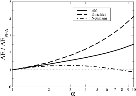
Figure 2: Ratio of the exact and PFA Casimir interaction energy differences $\Delta E=E_{12}-E^{\rm cc}_{12}$ between eccentric ($E_{12}$) and concentric ($E^{\rm cc}_{12}$) cylinders in the limit of small eccentricity $\epsilon\ll a$. The curve EM denotes the full electromagnetic Casimir energy.

We can also obtain the exact Casimir interaction energy for the cylinder-plane configuration Emig2006 as a limiting case of our exact results for eccentric cylinders Eq.(3). Indeed, the eccentric cylinder configuration tends to the cylinder-plane configuration for large values of both the eccentricity $\epsilon$ and the radius $b$ of the outer cylinder, keeping the radius $a$ of the inner cylinder and the distance $d$ between the cylinders fixed. Using the addition theorem and uniform expansions for Bessel functions it can be proved that, for $x\gg h$,

$$\sum_{m}\frac{K_{m}(x+h)}{I_{m}(x+h)}I_{n-m}(x)I_{p-m}(x)\approx K_{n+p}(2h),$$

$$\sum_{m}\frac{K^{\prime}_{m}(x+h)}{I^{\prime}_{m}(x+h)}I_{n-m}(x)I_{p-m}(x)\approx-K_{n+p}(2h).$$

Using these equations (with $x\equiv\beta\epsilon/a$ and $h\equiv\beta H/a$) in our exact formula the known result for the Casimir energy in the cylinder-plane configuration is obtained Emig2006

$$A_{np}^{\rm TM,c-p} = \frac{I_{n}(\beta)}{K_{n}(\beta)}\;K_{n+p}(2\beta H/a),$$

$$A_{np}^{\rm TE,c-p} = -\frac{I^{\prime}_{n}(\beta)}{K^{\prime}_{n}(\beta)}\;K_{n+p}(2\beta H/a).$$

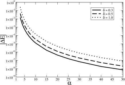
Figure 3: Exact interaction energy difference $|\Delta E|$ as a function of $\alpha$ for different values of $\delta$. Energies are measured in units of $\hbar cL/4\pi a^{2}$. These results interpolate between the $(\alpha-1)^{-5}$ behavior for $\alpha\rightarrow 1$, and the $(\alpha^{4}\log\alpha)^{-1}$ behavior for $\alpha\gg 1$.

We now focus on quasi-concentric cylinders, when the eccentricity is small as compared to the radius of the inner cylinder, i.e. $\delta\ll 1$. The ratio between the radii, $\alpha=b/a$, need not be close to unity, so that PFA is in general not valid in this configuration - as only for $\alpha\rightarrow 1$ do we expect to recover PFA. The zeroth order $\epsilon=0$ corresponds to the concentric case, where the matrices $A_{np}^{\rm TE,TM}$ are diagonal. This case was studied in Mazzitelli2003 by means of exact and semiclassical treatments, and it was shown that the PFA concentric energy goes as $E^{\rm cc}_{12}=-\hbar c\pi^{3}L/360a^{2}(\alpha-1)^{3}$. Obviously, symmetry arguments imply that there is no net Casimir force between the cylinders in the concentric configuration. To next order the correction to the energy, $\Delta E=E_{12}-E^{\rm cc}_{12}$, depends on $\epsilon^{2}$, leading to an unstable equilibrium position for the concentric geometry. The behavior of the Bessel functions for small eccentricity, $I_{m-n}(z)\simeq(z)^{n-m}$, suggests that one should use the tridiagonal version of the matrices $A_{np}^{\rm TE,TM}$ considering only elements with $p=n$ and $p=n\pm 1$. Expanding the determinants to order $O(\epsilon^{2})$, one can write the TM contribution as

$$\Delta E^{\rm TM} = -\frac{\hbar cL\epsilon^{2}}{4\pi a^{4}}\sum_{n=-\infty}^{\infty}\int_{0}^{\infty}d\beta\;\beta^{3}\;\frac{1}{1-{\cal D}^{\rm cc}_{n}}$$ (4)

$$\times\left[{\cal D}_{n}+\frac{{\cal N}_{n}}{1-{\cal D}^{\rm cc}_{n+1}}\right],$$

where ${\cal D}^{\rm cc}_{n}=I_{n}(\beta)K_{n}(\alpha\beta)/K_{n}(\beta)I_{n}(\alpha\beta)$ is the $\epsilon=0$, diagonal TM contribution, and ${\cal D}_{n}$ and ${\cal N}_{n}$ are the $O(\epsilon^{2})$ diagonal and non-diagonal TM contributions, respectively. They read

$${\cal D}_{n} = \frac{{\cal D}^{\rm cc}_{n}}{2}+\frac{I_{n}(\beta)}{4K_{n}(\beta)}\left[\frac{K_{n-1}(\alpha\beta)}{I_{n-1}(\alpha\beta)}+\frac{K_{n+1}(\alpha\beta)}{I_{n+1}(\alpha\beta)}\right],$$

$${\cal N}_{n} = \frac{I_{n}(\beta)I_{n+1}(\beta)}{4K_{n}(\beta)K_{n+1}(\beta)}\left[\frac{K_{n}(\alpha\beta)}{I_{n}(\alpha\beta)}+\frac{K_{n+1}(\alpha\beta)}{I_{n+1}(\alpha\beta)}\right]^{2}.$$

A similar expression holds for the TE contribution, with the Bessel functions replaced by their derivatives. Eq.(4) and the corresponding TE one are exact expressions for the Casimir energy difference between eccentric and concentric cases in the limit $\epsilon\ll a$.

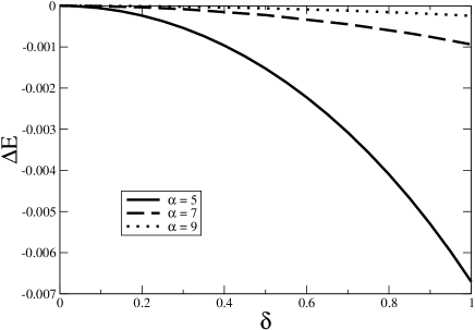
Figure 4: Exact interaction energy difference $\Delta E$ as a function of $\delta$ for different values of $\alpha$. Energies are measured in units of $\hbar cL/4\pi a^{2}$. The maximum at $\delta=0$ shows the instability of the equilibrium point.

The PFA limit $\Delta E^{\rm TE}_{\rm PFA}=\Delta E^{\rm TM}_{\rm PFA}=\Delta E^{\rm EM}_{\rm PFA}/2=-\pi^{3}\hbar cL\epsilon^{2}/240a^{4}(\alpha-1)^{5}$ can be obtained from Eq.(4) considering $\alpha\rightarrow 1$. In this limit the leading contribution arises from large values of the summation index $n$, for which the use of asymptotic uniform expansions of the Bessel functions is in order. Fig. 2 depicts the ratio of the exact Casimir energy $\Delta E$ and the PFA limit for the almost concentric cylinders configuration. As evident from the figure, PFA agrees with the exact result at a few percent level only for $\alpha$ very close to unity, and then it noticeably departs from the PFA prediction. In the opposite limit, $\alpha\rightarrow\infty$, the Dirichlet contribution is much larger than the Neumann one, and the integral and sum in Eq.(4) is dominated by the $n=0$ term. The asymptotic result for the energy is

$$\Delta E_{\infty} = -\frac{\hbar cL\epsilon^{2}}{8\pi a^{4}\alpha^{4}\log\alpha}\int_{0}^{\infty}d\beta\beta^{3}\left[\frac{K_{0}(\beta)}{I_{0}(\beta)}+\frac{K_{1}(\beta)}{I_{1}(\beta)}\right]$$ (5)

$$\approx -\frac{3.3348\hbar cL\epsilon^{2}}{8\pi a^{4}\alpha^{4}\log\alpha}.$$

This equation is valid when $\log\alpha\gg 1$. From Eq.(5) we see that the force between cylinders in the limit $a$, $\epsilon\ll b$ is proportional to $L\epsilon/b^{4}\ln(b/a)$. The weak logarithmic dependence on $\alpha$ is characteristic of the cylindrical geometry. A similar weak decay at large distances has been found for the cylinder-plane geometry Emig2006 .

Next we consider arbitrary values of the eccentricity. In this case we need to perform a numerical evaluation of the determinants in Eq.(3). We find that as $\alpha$ approaches smaller values, larger matrices are needed for ensuring convergence. Moreover, for increasing values of $\delta$ it is necessary to include more terms in the series defining the coefficients $A_{np}^{\rm TE,TM}$. In Fig. 3 we plot the interaction energy difference $|\Delta E|$ as a function of $\alpha$ for different values of $\delta$. These numerical results interpolate between the PFA and the asymptotic behavior for large $\alpha$, beyond the quasi-concentric limit. Fig. 4 shows the complementary information, with the Casimir energy as a function of $\delta$ for various values of $\alpha$, showing explicitly the instability of the concentric equilibrium position.

The exact evaluation of the Casimir force between parallel eccentric cylinders obtained here lends itself to a variety of applications for experiments implementing this geometry in the micrometer and the nanometer scales. Firstly, the accurate knowledge of the Casimir force in this configuration allows to look for extra-gravitational forces while the usual gravitational force, apart from border effects, is cancelled. The cancellation of the Newtonian gravitational force is also common to the parallel plate geometry if a dynamical measurement technique is adopted for the latter configuration, however in addition the concentric cylinder case has better shielding from the electrostatic force due to spurious charges, allowing for a null experiment with respect to both Newtonian and Coulombian background forces even with a static measurement technique. This suggests a micrometer version of experiments performed using the concentric cylinders configuration and a torsional balance to test the inverse-square gravitational law in the cm range Spero . In particular, in the case of a repulsive Yukawian force, one can envisage a situation where the unstable equilibrium due to the Casimir force is balanced or overcome by the former, and even the qualitative observation of mechanical stability in the concentric configuration will establish the existence of a new force. Secondly, the measurement of the Casimir force in various configurations involving cylinders (with the first example provided in Ederth2000 for crossed cylinders) is interesting in itself as one can make reliable tests of the PFA approximation versus both the exact solution and the actual experimental outcome. We expect that the case of two parallel cylinders with distance larger than the sum of their radii will experience stronger deviations between PFA and the exact solution. This case could be analyzed using the approach presented here. Thirdly, our results could lead to a quantitative explanation, once finite conductivity and temperature effects will be taken into account, for the observed easiness to bend laterally multiwall nanotubes. The Casimir force and its non-retarded counterpart Hertel provide a natural mechanism to allow for instability from the perfectly concentric situation of nanotubes, and could also play a role in the observed decrease of the effective bending modulus of nanotubes with large (tens to hundreds nm) radii Dresselhaus , and their fragmentation Wood .

The work of F.C.L. and F.D.M. is supported by UBA, Conicet and ANPCyT (Argentina).

References

- (1) H.B.G. Casimir, Proc. K. Ned. Akad. Wet. B 51, 793 (1948).
- (2) S.K. Lamoreaux, Phys. Rev. Lett. 78, 5 (1997).
- (3) U. Mohideen and A. Roy, Phys. Rev. Lett. 81, 4549 (1998).
- (4) T. Ederth, Phys. Rev. A 62, 062104 (2000).
- (5) H.B. Chan, V.A. Aksyuk, R.N. Kleiman, D.J. Bishop, and F. Capasso, Science 291, 1941 (2001).
- (6) G. Bressi, G. Carugno, R. Onofrio, and G. Ruoso, Phys. Rev. Lett. 88, 041804 (2002).
- (7) R.S. Decca, D. Lopez, E. Fischbach, and D.E. Krause, Phys. Rev. Lett. 91, 050402 (2003).
- (8) H.B. Chan, V.A. Aksyuk, R. N. Kleiman, D.J. Bishop, and F. Capasso, Phys. Rev. Lett. 87, 211801 (2001).
- (9) B.V. Derjaguin and I.I. Abrikosova, Sov. Phys. JETP 3, 819 (1957); B.V. Derjaguin, Sci. Am. 203, 47 (1960); J. Blocki, J. Randrup, W.J. Swiatecki, and C.F. Tsang, Ann. Phys. 105, 427 (1977).
- (10) M. Schaden and L. Spruch, Phys. Rev. Lett. 84, 459 (2000).
- (11) F.D. Mazzitelli, M.J. Sánchez, N.N. Scoccola, and J. von Stecher, Phys. Rev. A 67, 013807 (2003).
- (12) R.L. Jaffe and A. Scardicchio, Phys. Rev. Lett. 92, 070402 (2004).
- (13) H. Gies, K. Langfeld, and L. Moyaerts, JHEP 06, 018 (2003).
- (14) R.B. Rodrigues, P.A. Maia Neto, A. Lambrecht, and S. Reynaud, Phys. Rev. Lett. 96, 100402 (2006).
- (15) H. Gies and K. Klingmuller, Phys. Rev. Lett. 96, 220401 (2006).
- (16) A. Bulgac, P. Magierski, and A. Wirzba, Phys. Rev. D 73, 025007 (2006).
- (17) T. Emig, R.L. Jaffe, M. Kardar, and A. Scardicchio, Phys. Rev. Lett. 96, 080403 (2006); M. Bordag, arXiv:hep-th/0602295.
- (18) D.A.R. Dalvit, F.C. Lombardo, F.D. Mazzitelli, and R. Onofrio, Europhys. Lett. 67, 517 (2004).
- (19) M. Brown-Hayes, D.A.R. Dalvit, F.D. Mazzitelli, W.J. Kim, and R. Onofrio, Phys. Rev. A 72, 052102 (2005).
- (20) G.S. Singh and L.S. Kothari, J. Math. Phys. 25, 810 (1984).
- (21) J.A. Balseiro, Revista de la Union Matemática Argentina, v. XIV, 118 (1950).
- (22) A.A. Saharian and A.S. Tarloyan, arXiv:hep-th/0603144.
- (23) R. Spero, J.K. Hoskins, R. Newman, J. Pellam, and J. Schultz, Phys. Rev. Lett. 44, 1645 (1980).
- (24) T. Hertel, R.E. Walkup, and P. Avouris, Phys. Rev. B 58, 13870 (1998); J. Cumings and A. Zetti, Science 289, 602 (2000); C.Q. Ru, Phys. Rev. B 62, 16962 (2000).
- (25) M.S. Dresselhaus, G. Dresselhaus, J.C. Charlier, and E. Hernández, Phil. Trans. R. Soc. Lond. A 362, 2065 (2004).
- (26) J.R. Wood, H.D. Wagner, and G. Marom, Proc. R. Soc. Lond. A 452, 235 (1996); H.D. Wagner, O. Lourie, Y. Feldman, and R. Tenne, Appl. Phys. Lett. 72, 188 (1998).