Catalytic quantum error correction

Abstract

We develop the theory of entanglement-assisted quantum error correcting (EAQEC) codes, a generalization of the stabilizer formalism to the setting in which the sender and receiver have access to pre-shared entanglement. Conventional stabilizer codes are equivalent to dual-containing symplectic codes. In contrast, EAQEC codes do not require the dual-containing condition, which greatly simplifies their construction. We show how any quaternary classical code can be made into a EAQEC code. In particular, efficient modern codes, like LDPC codes, which attain the Shannon capacity, can be made into EAQEC codes attaining the hashing bound. In a quantum computation setting, EAQEC codes give rise to catalytic quantum codes which maintain a region of inherited noiseless qubits. We also give an alternative construction of EAQEC codes by making classical entanglement assisted codes coherent.

Information theory and the theory of error-correcting codes (coding theory) are intimately connected. Both address the problem of sending information over noisy channels. The sender Alice encodes her message as a codeword, sends it through the channel, and the receiver Bob tries to infer the intended message based on the channel output.

Information theory (or rather the subfield of Shannon theory) deals with the asymptotic setting of increasingly long codes, with asymptotically vanishing error probability. The noisy channel is typically assumed to act independently on the codeword bits. The fundamental quantity of interest is the capacity of the channel: the optimal rate (in bits per channel use) of information transfer. Claude Shannon [30] gave a remarkable characterization of the channel capacity in terms of mutual information. Unfortunately, the capacity is achieved by random coding, which means highly inefficient encoding and decoding algorithms.

Coding theory deals with the practical finite setting, characterized by a fixed code length, number of encoded bits and correctable error set. The most popular codes have simple mathematical properties, such as linearity (a linear combination of codewords is another codeword), which allows for efficient encoding. The performance of these codes is then measured against the optimal performance set by Shannon theory.

This relationship carries over to quantum information processing. The basic communication task is sending quantum information over noisy quantum channels. This setting is also relevant for fault tolerant quantum computation, because decoherence can be regarded as a quantum channel connecting two points in time (rather than space). The first quantum error-correcting (QEC) code was discovered by Shor [31], leading to an explosion of research in subsequent years [16, 2, 22, 21, 33, 9, 17, 7, 8]. Calderbank and Shor [9] and Steane [33] gave the first systematic way to construct quantum “CSS” codes from dual-containing classical codes over $\mathbb{Z}_{2}$. These efforts culminated in a general theory of linear quantum codes, also known as stabilizer codes [8, 17, 29, 28]. Stabilizer codes are equivalent to classical codes which are dual-containing with respect to the symplectic bilinear form. These in turn may be constructed from dual-containing classical codes over $\mathbb{F}_{4}$, generalizing the CSS construction [7].

In [31] Shor also raised the information theoretical question of characterizing the capacity of a quantum channel for sending quantum information, subsequently answered by [23, 32, 11] in terms of coherent information. It comes as no surprise that coding theory and information theory continue to inform each other in the quantum setting. The capacity-achieving quantum codes of [11] have a structure akin to CSS codes (thanks to their common connection to cryptography). Concatenated stabilizer codes achieve rates equal to the coherent information evaluated on density operators corresponding to maximally mixed qubit states encoded by a stablizer code [2, 18].

Research has since taken us beyond this most obvious quantum communication setting. Apart from quantum communication channels, there are other resources to consider, such as entanglement and classical communication. Great progress has been made in characterizing optimal tradeoffs between these resources. For example, the capacity of a quantum channel for sending classical information assisted by entanglement (EA capacity) is a simple single letter expression involving quantum mutual information [3]. In [13] a remarkable duality was discovered between entanglement-assisted quantum communication (the “father” protocol) and quantum-communication-assisted entanglement distillation (the “mother” protocol). The two were shown to generate a whole family of protocols when combined with the more elementary protocols of superdense coding [4], quantum teleportation [1] and entanglement distribution [13].

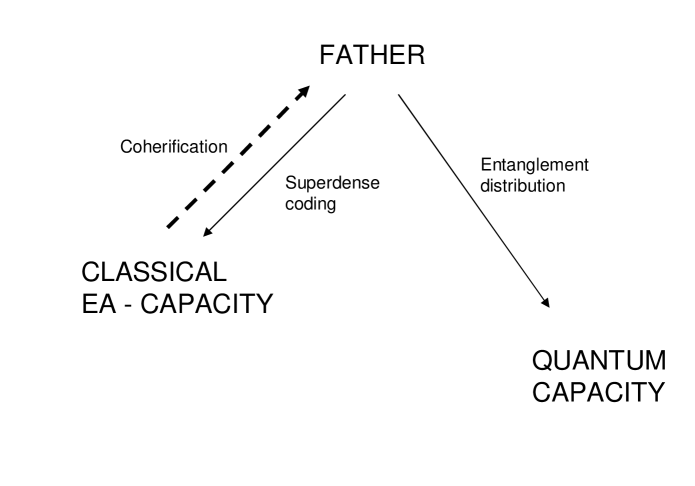
Figure 1: The male side of the family tree of quantum Shannon theory [13].

The father side of the family is shown in Figure 1. Quantum capacity-achieving protocols can be obtained from the father protocol by combining it with entanglement distribution. In conjunction with superdense coding, the father protocol gives rise to EA capacity-achieving protocols. Moreover, the latter can be made coherent [19, 11, 13, 12] to recover the father protocol.

Can we reproduce the family in the finite setting of coding theory? Is it beneficial to do so? In this paper we give an affirmative answer to these two questions. We develop a general theory of linear “father” codes or entanglement-assisted quantum error-correcting (EAQEC) codes. The first and only such code to date was constructed by Bowen [5] from the $[[5,1,3]]$ QEC code. EAQEC codes turn out to be a rather natural generalization of the usual stabilizer codes, equivalent to classical symplectic codes. These codes need not be dual-containing: the degree to which they are not measures the required amount of entanglement assistance. Consequently, any classical code can be made into a EAQEC code. This provides a drastic simplification, allowing the classical theory of error correction to be imported wholesale.

The paper is organized as follows. Section 1 provides background on the Pauli group and symplectic algebra. It also reviews basic quantum strategies for sending classical information. Section 2 defines EAQEC codes and determines the set of errors they can correct. Section 3 generalizes the code construction method of [7, 8] based on classical codes over $\mathbb{F}_{4}$. Section 4 regards the right branch of Figure 1: constructing catalytic QEC codes from EAQEC codes. Section 5 regards the left branch of Figure 1: constructing entanglement assisted codes for sending classical information (EACEC codes). These are then made coherent [12], providing an alternative construction of EAQEC codes. Section 6 discusses bounds on the performance of EAQEC codes. Section 7 recovers Bowen’s result in our framework. Section 8 updates the table of known codes from [8]. We discuss our results in Section 9.

1 Background

In this section we review the properties of Pauli matrices, and relate them to symplectic binary and quaternary vector spaces. Our presentation follows Forney et al. [20] and Hamada [18].

1.1 Single qubit Pauli group

A qubit is a quantum system corresponding to a two dimensional complex Hilbert space ${\cal H}$. Fixing a basis for ${\cal H}$, the set $\Pi$ of Pauli matrices is defined as

$$I=\left[\begin{array}[]{cc}1&0\\ 0&1\end{array}\right],\quad X=\left[\begin{array}[]{cc}0&1\\ 1&0\end{array}\right],\quad Y=\left[\begin{array}[]{cc}0&-i\\ i&0\end{array}\right],\quad Z=\left[\begin{array}[]{cc}1&0\\ 0&-1\end{array}\right].$$

The Pauli matrices are Hermitian unitary matrices with eigenvalues belonging to the set $\{1,-1\}$. The multiplication table of these matrices is given by:

$$\begin{array}[]{|c|cccc|}\hline\cr\times&I&X&Y&Z\\ \hline\cr I&I&X&Y&Z\\ X&X&I&iZ&-iY\\ Y&Y&-iZ&I&iX\\ Z&Z&iY&-iX&I\\ \hline\cr\end{array}$$

Observe that the Pauli matrices either commute or anticommute. Let $[A]=\{\beta A\mid\beta\in\mathbb{C},|\beta|=1\}$ be the equivalence class of matrices equal to $A$ up to a phase factor. Then the set $[\Pi]=\{[I],[X],[Y],[Z]\}$ is readily seen to form a commutative group under the multiplication operation defined by $[A][B]=[AB]$. It is called the Pauli group.

We are interested in relating the Pauli group to the additive group $(\mathbb{Z}_{2})^{2}=\{00,01,10,11\}$ of binary words of length $2$ described by the table:

$$\begin{array}[]{|c|cccc|}\hline\cr+&00&01&11&10\\ \hline\cr 00&00&01&11&10\\ 01&01&00&10&11\\ 11&11&10&00&01\\ 10&10&11&01&00\\ \hline\cr\end{array}$$

This group is also a two-dimensional vector space over the field $\mathbb{Z}_{2}$. A bilinear form can be defined over this vector space, called the symplectic form or symplectic product $\odot:(\mathbb{Z}_{2})^{2}\times(\mathbb{Z}_{2})^{2}\rightarrow\mathbb{Z}_{2}$, given by the table

$$\begin{array}[]{|c|cccc|}\hline\cr\odot&00&01&11&10\\ \hline\cr 00&0&0&0&0\\ 01&0&0&1&1\\ 11&0&1&0&1\\ 10&0&1&1&0\\ \hline\cr\end{array}$$

In what follows we will often write elements of $(\mathbb{Z}_{2})^{2}$ as $u=(z|x)$, with $z,x\in\mathbb{Z}_{2}$. For instance, $01$ becomes $(0|1)$. For $u=(z|x),v=(z^{\prime}|x^{\prime})\in(\mathbb{Z}_{2})^{2}$ the symplectic product is equivalently defined by

$$u\odot v=zx^{\prime}-z^{\prime}x.$$

Define the map $N:(\mathbb{Z}_{2})^{2}\to\Pi$ by the following table:

$$\begin{array}[]{|c|c|}\hline\cr(\mathbb{Z}_{2})^{2}&\Pi\\ \hline\cr 00&I\\ 01&X\\ 11&Y\\ 10&Z\\ \hline\cr\end{array}$$

This map is defined in such a way that $N_{(z|x)}$ and $Z^{z}X^{x}$ are equal up to a phase factor, i.e.

$$[N_{(z|x)}]=[Z^{z}X^{x}].$$

We make two key observations

1. The map $[N]:(\mathbb{Z}_{2})^{2}\to[\Pi]$ induced by $N$ is an isomorphism:

   $$[N_{u}][N_{v}]=[N_{u+v}].$$

2. The commutation relations of the Pauli matrices are captured by the symplectic product

   $$N_{u}N_{v}=(-1)^{u\odot v}N_{v}N_{u}.$$

Both properties are readily verified from the tables.

1.2 Multi-qubit Pauli group

Consider an $n$-qubit system corresponding to the tensor product Hilbert space ${\cal H}^{\otimes n}$. Define an $n$-qubit Pauli matrix ${\mathbf{A}}$ to be of the form ${\mathbf{A}}=A_{1}\otimes A_{2}\otimes\cdots\otimes A_{n}$, where $A_{j}\in\Pi$. The set of all $4^{n}$ $n$-qubit Pauli matrices is denoted by $\Pi^{n}$. The product of elements of $\Pi^{n}$ is an element of $\Pi^{n}$ up to a phase factor. Define as before the equivalence class $[{\mathbf{A}}]=\{\beta{\mathbf{A}}\mid\beta\in\mathbb{C},|\beta|=1\}$. Then

$$[{\mathbf{A}}][{\mathbf{B}}]=[A_{1}B_{1}]\otimes[A_{2}B_{2}]\otimes\cdots\otimes[A_{n}B_{n}]=[{\mathbf{A}}{\mathbf{B}}].$$

Thus the set $[\Pi^{n}]=\{[{\mathbf{A}}]:{\mathbf{A}}\in\Pi^{n}\}$ is a commutative multiplicative group.

Now consider the group/vector space $(\mathbb{Z}_{2})^{2n}$ of binary vectors of length $2n$. Its elements may be written as ${\mathbf{u}}=({\mathbf{z}}|{\mathbf{x}})$, ${\mathbf{z}}=z_{1}\dots z_{n}\in(\mathbb{Z}_{2})^{n}$, ${\mathbf{x}}=x_{1}\dots x_{n}\in(\mathbb{Z}_{2})^{n}$. We shall think of ${\mathbf{u}}$, ${\mathbf{z}}$ and ${\mathbf{x}}$ as row vectors. The symplectic product of ${\mathbf{u}}=({\mathbf{z}}|{\mathbf{x}})$ and ${\mathbf{v}}=({\mathbf{z}}^{\prime}|{\mathbf{x}}^{\prime})$ is given by

$${\mathbf{u}}\odot{\mathbf{v}}^{{{T}}}={\mathbf{z}}\,{{\mathbf{x}}^{\prime}}^{{{T}}}-{\mathbf{z}}^{\prime}\,{\mathbf{x}}^{{{T}}}.$$

The right hand side are binary inner products and $T$ denotes the transpose. This should be thought of as a kind of matrix multiplication of a row vector and a column vector. We use ${\mathbf{u}}\odot{\mathbf{v}}^{{{T}}}$ rather than the more standard ${\mathbf{u}}\,{\mathbf{v}}^{{T}}$ to emphasize that the symplectic form is used rather than the binary inner product. Equivalently,

$${\mathbf{u}}\odot{\mathbf{v}}^{{T}}=\sum_{i}u_{i}\odot v_{i}$$

where $u_{i}=(z_{i}|x_{i}),v_{i}=(z^{\prime}_{i}|x^{\prime}_{i})$ and this sum represents Boolean addition. Observe that ${{\mathbf{u}}}\odot{{\mathbf{u}}}^{{T}}=0$, i.e., every vector is “orthogonal” to itself.

The map $N:(\mathbb{Z}_{2})^{2n}\rightarrow\Pi^{n}$ is now defined as

$$N_{\mathbf{u}}=N_{u_{1}}\otimes\dots\otimes N_{u_{n}}.$$

Writing

$$X^{{\mathbf{x}}}=X^{x_{1}}\otimes\dots\otimes X^{x_{n}},$$

$$Z^{{\mathbf{z}}}=Z^{z_{1}}\otimes\dots\otimes Z^{z_{n}},$$

as in the single qubit case, we have

$$[N_{({\mathbf{z}}|{\mathbf{x}})}]=[Z^{{\mathbf{z}}}X^{{\mathbf{x}}}].$$

The two observations made for the single qubit case also hold:

1. The map $[N]:(\mathbb{Z}_{2})^{2n}\to[\Pi^{n}]$ induced by $N$ is an isomorphism:

   $$[N_{\mathbf{u}}][N_{\mathbf{v}}]=[N_{{\mathbf{u}}+{\mathbf{v}}}].$$ (1)

   Consequently, if $\{{\mathbf{u}}_{1},\dots,{\mathbf{u}}_{m}\}$ is a linearly independent set then the elements of the Pauli group subset $\{[N_{{\mathbf{u}}_{1}}],\dots,[N_{{\mathbf{u}}_{m}}]\}$ are independent in the sense that no element can be written as a product of others.

2. The commutation relations of the $n$-qubit Pauli matrices are captured by the symplectic product

   $$N_{\mathbf{u}}N_{\mathbf{v}}=(-1)^{{\mathbf{u}}\odot{\mathbf{v}}^{{T}}}N_{\mathbf{v}}N_{\mathbf{u}}.$$ (2)

1.3 Properties of the symplectic form

In this subsection we present two results which will play a major role in the construction of EAQEC codes. Together they will enable us to conclude that any independent subset of the $n$-qubit Pauli group can be transformed via a unitary operation into a canonical set whose elements act nontrivially only on single qubits.

A subspace $V$ of $(\mathbb{Z}_{2})^{2n}$ is called symplectic [10] if there is no ${\mathbf{v}}\in V$ such that

$${\mathbf{v}}\odot{\mathbf{u}}^{{T}}=0,\,\,\,\forall{\mathbf{u}}\in V.$$ (3)

$(\mathbb{Z}_{2})^{2n}$ is itself a symplectic subspace. Consider the standard basis for $(\mathbb{Z}_{2})^{2n}$, consisting of ${\mathbf{g}}_{i}=({\mathbf{e}}_{i}|{\mathbf{0}})$ and ${\mathbf{h}}_{i}=({\mathbf{0}}|{\mathbf{e}}_{i})$ for $i=1,\dots,n$, where ${\mathbf{e}}_{i}=(0,\dots,0,1,0,\dots,0)$ [$1$ in the $i$th position] are the standard basis vectors of $(\mathbb{Z}_{2})^{n}$. Observe that

$${\mathbf{g}}_{i}\odot{\mathbf{g}}_{j}^{{T}}=0, {\rm for\,\,all\,\,}i,j$$ (4)

$${\mathbf{h}}_{i}\odot{\mathbf{h}}_{j}^{{T}}=0, {\rm for\,\,all\,\,}i,j$$ (5)

$${\mathbf{g}}_{i}\odot{\mathbf{h}}_{j}^{{T}}=0, {\rm for\,\,all\,\,}i\neq j$$ (6)

$${\mathbf{g}}_{i}\odot{\mathbf{h}}_{i}^{{T}}=1, {\rm for\,\,all\,\,}i.$$ (7)

Thus, the basis vectors come in $n$ hyperbolic pairs $({\mathbf{g}}_{i},{\mathbf{h}}_{i})$ such that only the symplectic product between hyperbolic partners is nonzero. The matrix $J=[{\mathbf{g}}_{i}\odot{\mathbf{h}}_{j}^{{T}}]$ defining the symplectic product with respect to this basis is given by

$$J=\left(\begin{array}[]{cc}0_{n\times n}&I_{n\times n}\\ I_{n\times n}&0_{n\times n}\end{array}\right),$$ (8)

where $I_{n\times n}$ and $0_{n\times n}$ are the $n\times n$ identity and zero matrices, respectively. A basis for $(\mathbb{Z}_{2})^{2n}$ whose symplectic product matrix $J$ is given by (8) is called a symplectic basis. In the Pauli picture, the hyperbolic pairs $({\mathbf{g}}_{i},{\mathbf{h}}_{i})$ correspond to $(Z^{{\mathbf{e}}_{i}},X^{{\mathbf{e}}_{i}})$ – the anticommuting $Z$ and $X$ Pauli matrices acting on the $i$th qubit.

In contrast, a subspace $V$ of $(\mathbb{Z}_{2})^{2n}$ is called isotropic if (3) holds for all ${\mathbf{v}}\in V$. The largest isotropic subspace of $(\mathbb{Z}_{2})^{2n}$ is $n$-dimensional. The span of the ${\mathbf{g}}_{i}$, $i=1,\dots,n$, is an example of a subspace saturating this bound.

A general subspace of $(\mathbb{Z}_{2})^{2n}$ is neither symplectic nor isotropic. The following theorem, stated in [10] and rediscovered in Pauli language in [15], says that an arbitrary subspace $V$ can be decomposed as a direct sum of a symplectic part and an isotropic part. We give an independent proof here.

Theorem 1.1

Let $V$ be an $m$-dimensional subspace of $(\mathbb{Z}_{2})^{2n}$. Then there exists a symplectic basis of $(\mathbb{Z}_{2})^{2n}$ consisting of hyperbolic pairs $({\mathbf{u}}_{i},{\mathbf{v}}_{i})$, $i=1,\dots,n$, such that $\{{\mathbf{u}}_{1},\dots,{\mathbf{u}}_{c+\ell},{\mathbf{v}}_{1},\dots,{\mathbf{v}}_{c}\}$ is a basis for $V$, for some $c,\ell\geq 0$ with $2c+\ell=m$.

Equivalently,

$$V={\rm symp}(V)\oplus{\rm iso}(V)$$

where ${\rm symp}(V)={\rm span}\{{\mathbf{u}}_{1},\dots,{\mathbf{u}}_{c},{\mathbf{v}}_{1},\dots,{\mathbf{v}}_{c}\}$ is symplectic and ${\rm iso}(V)={\rm span}\{{\mathbf{u}}_{c+1},\dots,{\mathbf{u}}_{c+\ell}\}$ is isotropic.

Remark   It is readily seen that the space ${\rm iso}(V)$ is unique, given $V$. In contrast, ${\rm symp}(V)$ is not. For instance, replacing ${\mathbf{v}}_{1}$ by ${\mathbf{v}}_{1}^{\prime}={\mathbf{v}}_{1}+{\mathbf{u}}_{c+1}$ in the above definition of ${\rm symp}(V)$ does not change its symplectic property.

Proof  Pick an arbitrary basis $\{{\mathbf{w}}_{1},\dots,{\mathbf{w}}_{m}\}$ for $V$ and extend it to a basis $\{{\mathbf{w}}_{1},\dots,{\mathbf{w}}_{2n}\}$ for $(\mathbb{Z}_{2})^{2n}$. We will describe an algorithm which yields the basis from the statement of the theorem.

The procedure consists of $n$ rounds. In each round a new hyperbolic pair $({\mathbf{u}}_{i},{\mathbf{v}}_{i})$ is generated; the index $i$ is added to the set ${\cal U}$ $({\cal V})$ if ${\mathbf{u}}_{i}\in V$ (${\mathbf{v}}_{i}\in V$).

Initially set $i=1$, $m^{\prime}=m$, and ${\cal U}={\cal V}=\emptyset$. The $i$th round reads as follows.

1. We start with vectors ${\mathbf{w}}_{1},\dots,{\mathbf{w}}_{2(n-i+1)}$, and ${\mathbf{u}}_{1},\dots\mathbf{u}_{i-1},{\mathbf{v}}_{1},\dots\mathbf{v}_{i-1}$, such that

   1. ${\mathbf{w}}_{1},\dots,{\mathbf{w}}_{2(n-i+1)},$ ${\mathbf{u}}_{1},\dots\mathbf{u}_{i-1},$${\mathbf{v}}_{1},\dots\mathbf{v}_{i-1}$ is a basis for $(\mathbb{Z}_{2})^{2n}$,

   2. each of ${\mathbf{u}}_{1},\dots\mathbf{u}_{i-1},{\mathbf{v}}_{1},\dots\mathbf{v}_{i-1}$ has vanishing symplectic product with each of ${\mathbf{w}}_{1},\dots,{\mathbf{w}}_{2(n-i+1)}$,

   3. $V={\rm span}\{{\mathbf{w}}_{j}:1\leq j\leq m^{\prime}\}\oplus{\rm span}\{{\mathbf{u}}_{j}:j\in{\cal U}\}\oplus{\rm span}\{{\mathbf{v}}_{j}:j\in{\cal V}\}$.

   These conditions are satisfied for $i=1$.

2. Define ${\mathbf{u}}_{i}={\mathbf{w}}_{1}$. If $m^{\prime}\geq 1$ then and add $i$ to ${\cal U}$. Let $j\geq 2$ be the smallest index for which ${\mathbf{w}}_{1}\odot{\mathbf{w}}_{j}^{{T}}=1$. Such a $j$ exists because of (a), (b) and the fact that there exists a ${\mathbf{w}}\in(\mathbb{Z}_{2})^{2n}$ such that ${{\mathbf{u}}_{i}}\odot{{\mathbf{w}}}^{{T}}=1$.

   Set ${\mathbf{v}}_{i}={\mathbf{w}}_{j}$.

3. If $j\leq m^{\prime}$:

   This means that there is a hyperbolic partner of ${\mathbf{u}}_{i}$ in $V$. Add $i$ to ${\cal V}$; swap ${\mathbf{w}}_{j}$ with ${\mathbf{w}}_{2}$; for $k=3,\dots,2(n-i+1)$ perform

   $${\mathbf{w}}^{\prime}_{k-2}:={\mathbf{w}}_{k}-({\mathbf{v}}_{i}\odot{\mathbf{w}}_{k}^{{T}}){\mathbf{u}}_{i}-({\mathbf{u}}_{i}\odot{\mathbf{w}}_{k}^{{T}}){\mathbf{v}}_{i},$$

   so that

   $${\mathbf{w}}^{\prime}_{k-2}\odot{\mathbf{u}}_{i}^{{T}}={\mathbf{w}}^{\prime}_{k-2}\odot{\mathbf{v}}_{i}^{{T}}=0;$$ (9)

   set $m^{\prime}:=m^{\prime}-2$.

   If $j>m^{\prime}$:

   This means that there is no hyperbolic partner of ${\mathbf{u}}_{i}$ in $V$. Swap ${\mathbf{w}}_{j}$ with ${\mathbf{w}}_{2(n-i+1)}$; for $k=2,\dots,2(n-i)+1$ perform

   $${\mathbf{w}}^{\prime}_{k-1}:={\mathbf{w}}_{k}-({\mathbf{v}}_{i}\odot{\mathbf{w}}_{k}^{{T}}){\mathbf{u}}_{i}-({\mathbf{u}}_{i}\odot{\mathbf{w}}_{k}^{{T}}){\mathbf{v}}_{i},$$

   so that

   $${\mathbf{w}}^{\prime}_{k-1}\odot{\mathbf{u}}_{i}^{{T}}={\mathbf{w}}^{\prime}_{k-1}\odot{\mathbf{v}}_{i}^{{T}}=0;$$ (10)

   if $m^{\prime}\geq 1$ then set $m^{\prime}:=m^{\prime}-1$.

4. Let ${\mathbf{w}}_{k}:={\mathbf{w}}^{\prime}_{k}$ for $1\leq k\leq 2(n-i)$. We need to show that the conditions from item 1 are satisfied for the next round ($i:=i+1$). Condition (a) holds because $\{{\mathbf{u}}_{i},{\mathbf{v}}_{i},{\mathbf{w}}^{\prime}_{1},\dots\mathbf{w}^{\prime}_{2(n-i)}\}$ are related to the old $\{{\mathbf{w}}_{1},\dots\mathbf{w}_{2(n-i+1)}\}$ by an invertible linear transformation. Condition (b) follows from (9) and (10). Regarding condition (c), if $m^{\prime}=0$ then it holds because ${\cal U}$ and ${\cal V}$ did not change from the previous round. Otherwise, consider the two cases in item 3. If $j\leq m^{\prime}$ then $\{{\mathbf{u}}_{i},{\mathbf{v}}_{i},{\mathbf{w}}^{\prime}_{1},\dots\mathbf{w}^{\prime}_{m^{\prime}-2}\}$ are related to the old $\{{\mathbf{w}}_{1},\dots\mathbf{w}_{m^{\prime}}\}$ by an invertible linear transformation. If $j>m^{\prime}$ then $\{{\mathbf{u}}_{i},{\mathbf{w}}^{\prime}_{1},\dots\mathbf{w}^{\prime}_{m^{\prime}-1}\}$ are related to the old $\{{\mathbf{w}}_{1},\dots\mathbf{w}_{m^{\prime}}\}$ by an invertible linear transformation (the $({\mathbf{u}}_{i}\odot{\mathbf{w}}_{k}^{{T}}){\mathbf{v}}_{i}$ terms vanish for $1\leq k\leq m^{\prime}$ because there is no hyperbolic partner of ${\mathbf{u}}_{i}$ in $V$).

$0\leq m^{\prime}\leq 2(n-i)$ at the end of the $i$th round. Thus $m^{\prime}=0$ after $n$ rounds and hence $V={\rm span}\{{\mathbf{u}}_{j}:j\in{\cal U}\}\oplus{\rm span}\{{\mathbf{v}}_{j}:j\in{\cal V}\}$. The theorem follows by suitably reordering the $({\mathbf{u}}_{j},{\mathbf{v}}_{j})$. $\Box$

A symplectomorphism $\Upsilon:(\mathbb{Z}_{2})^{2n}\rightarrow(\mathbb{Z}_{2})^{2n}$ is a linear isomorphism which preserves the symplectic form, namely

$$\Upsilon({\mathbf{u}})\odot\Upsilon({\mathbf{v}})^{{T}}={\mathbf{u}}\odot{\mathbf{v}}^{{T}}.$$ (11)

The following theorem relates symplectomorphisms on $(\mathbb{Z}_{2})^{2n}$ to unitary maps on ${\cal H}^{\otimes n}$. It appears, for instance, in [6]. For completeness, we give an independent proof here.

Theorem 1.2

For any symplectomorphism $\Upsilon$ on $(\mathbb{Z}_{2})^{2n}$ there exists a unitary map $U_{\Upsilon}$ on ${\cal H}^{\otimes n}$ such that for all ${\mathbf{u}}\in(\mathbb{Z}_{2})^{2n}$,

$$[N_{\Upsilon({\mathbf{u}})}]=[U_{\Upsilon}N_{{\mathbf{u}}}U_{\Upsilon}^{-1}].$$

Remark.  The unitary map $U_{\Upsilon}$ may be viewed as a map on $[\Pi]$ given by $[{\mathbf{A}}]\mapsto[U_{\Upsilon}{\mathbf{A}}U_{\Upsilon}^{-1}]$. The theorem says that the following diagram commutes

$$\begin{CD}(\mathbb{Z}_{2})^{2n}@>{{\Upsilon}}>{}>(\mathbb{Z}_{2})^{2n}\\ @V{{[N]}}V{}V@V{}V{{[N]}}V\\ [\Pi]@>{U_{\Upsilon}}>{}>[\Pi]\end{CD}$$

Proof  Consider the standard basis ${\mathbf{g}}_{i}=({\mathbf{e}}_{i}|{\mathbf{0}})$, ${\mathbf{h}}_{i}=({\mathbf{0}}|{\mathbf{e}}_{i})$. Define the unique (up to a phase factor) state $|{\mathbf{0}}\rangle$ on ${\cal H}^{\otimes n}$ to be the simultaneous $+1$ eigenstate of the commuting operators $N_{{\mathbf{g}}_{j}}$, $j=1,\dots,n$. Define an orthonormal basis $\{|{\mathbf{b}}\rangle:{\mathbf{b}}=b_{1}\dots b_{n}\in(\mathbb{Z}_{2})^{n}\}$ for ${\cal H}^{\otimes n}$ by

$$|{\mathbf{b}}\rangle=N_{\sum_{i}b_{i}{\mathbf{h}}_{i}}|{\mathbf{0}}\rangle.$$

The orthonormality follows from the observation that $|{\mathbf{b}}\rangle$ is a simultaneous eigenstate of $N_{{\mathbf{g}}_{j}}$, $j=1,\dots,n$ with respective eigenvalues $(-1)^{b_{j}}$:

$$\begin{split}N_{{\mathbf{g}}_{j}}|{\mathbf{b}}\rangle&=N_{{\mathbf{g}}_{j}}N_{\sum_{i}b_{i}{\mathbf{h}}_{i}}|{\mathbf{0}}\rangle\\ &=(-1)^{b_{j}}N_{\sum_{i}b_{i}{\mathbf{h}}_{i}}N_{{\mathbf{g}}_{j}}|{\mathbf{0}}\rangle\\ &=(-1)^{b_{j}}N_{\sum_{i}b_{i}{\mathbf{h}}_{i}}|{\mathbf{0}}\rangle\\ &=(-1)^{b_{j}}|{\mathbf{b}}\rangle.\end{split}$$ (12)

The second line is an application of (2).

Define $\widetilde{{\mathbf{g}}}_{i}:=\Upsilon({\mathbf{g}}_{i})$. We repeat the above construction for this new basis. Define the unique (up to a phase factor) state ${|\widetilde{{\mathbf{0}}}\rangle}$ to be the simultaneous $+1$ eigenstate of the commuting operators $N_{\widetilde{{\mathbf{g}}}_{i}}$, $i=1,\dots,n$. Define an orthonormal basis $\{{|\widetilde{{\mathbf{b}}}\rangle}\}$ by

$$|\widetilde{{\mathbf{b}}}\rangle=N_{\sum_{i}b_{i}\widetilde{{\mathbf{h}}}_{i}}|\widetilde{{\mathbf{0}}}\rangle.$$ (13)

Defining ${\mathbf{u}}=\sum_{i}z_{i}{\mathbf{g}}_{i}+x_{i}{\mathbf{h}}_{i}$, $\widetilde{{\mathbf{u}}}=\sum_{i}z_{i}\widetilde{{\mathbf{g}}}_{i}+x_{i}\widetilde{{\mathbf{h}}}_{i}$ and ${\mathbf{x}}=x_{1}\dots x_{n}$, we have

$$\begin{split}N_{\widetilde{{\mathbf{u}}}}|\widetilde{{\mathbf{b}}}\rangle&=N_{\widetilde{{\mathbf{u}}}}N_{\sum_{i}b_{i}\widetilde{{\mathbf{h}}}_{i}}{|\widetilde{{\mathbf{0}}}\rangle}\\ &=(-1)^{\widetilde{{\mathbf{u}}}\odot(\sum_{i}b_{i}\widetilde{{\mathbf{h}}}_{i})^{{T}}}N_{\sum_{i}b_{i}\widetilde{{\mathbf{h}}}_{i}}N_{\widetilde{{\mathbf{u}}}}{|\widetilde{{\mathbf{0}}}\rangle}\\ &=(-1)^{\widetilde{{\mathbf{u}}}\odot(\sum_{i}b_{i}\widetilde{{\mathbf{h}}}_{i})^{{T}}}e^{i\theta(\widetilde{{\mathbf{u}}})}N_{\sum_{i}b_{i}\widetilde{{\mathbf{h}}}_{i}}N_{\sum_{i}x_{i}\widetilde{{\mathbf{h}}}_{i}}N_{\sum_{i}z_{i}\widetilde{{\mathbf{g}}}_{i}}{|\widetilde{{\mathbf{0}}}\rangle}\\ &=(-1)^{\widetilde{{\mathbf{u}}}\odot(\sum_{i}b_{i}\widetilde{{\mathbf{h}}}_{i})^{{T}}}e^{i\theta(\widetilde{{\mathbf{u}}})}N_{\sum_{i}(b_{i}+x_{i})\widetilde{{\mathbf{h}}}_{i}}{|\widetilde{{\mathbf{0}}}\rangle}\\ &=(-1)^{\widetilde{{\mathbf{u}}}\odot(\sum_{i}b_{i}\widetilde{{\mathbf{h}}}_{i})^{{T}}}e^{i\theta(\widetilde{{\mathbf{u}}})}{|\widetilde{{\mathbf{b}}+{\mathbf{x}}}\rangle}\\ &=(-1)^{{{\mathbf{u}}}\odot(\sum_{i}b_{i}{{\mathbf{h}}}_{i})^{{T}}}e^{i\theta(\widetilde{{\mathbf{u}}})}{|\widetilde{{\mathbf{b}}+{\mathbf{x}}}\rangle},\end{split}$$ (14)

where $\theta(\widetilde{{\mathbf{u}}})$ is a phase factor which is independent of ${\mathbf{b}}$. The first equality follows from (13), the second from (2), the third from (1), the fourth from the definition of $|\widetilde{{\mathbf{0}}}\rangle$ and the fact that $X^{{\mathbf{b}}}X^{{\mathbf{x}}}=X^{{\mathbf{b}}+{\mathbf{x}}}$, the fifth from (13), and the sixth from (11). Similarly

$$N_{\mathbf{u}}|{\mathbf{b}}\rangle=(-1)^{{{\mathbf{u}}}\odot(\sum_{i}b_{i}{{\mathbf{h}}}_{i})^{{T}}}e^{i\varphi({{\mathbf{u}}})}{|{{\mathbf{b}}+{\mathbf{x}}}\rangle},$$ (15)

where $\varphi({\mathbf{u}})$ is a is a phase factor which is independent of ${\mathbf{b}}$.

Define $U_{\Upsilon}$ by the change of basis

$$U_{\Upsilon}=\sum_{\mathbf{b}}|\widetilde{{\mathbf{b}}}\rangle\langle{{\mathbf{b}}}|.$$

Combining (14) and (15) gives for all $|{\mathbf{b}}\rangle$

$$\begin{split}N_{\Upsilon({\mathbf{u}})}U_{\Upsilon}|{\mathbf{b}}\rangle&=(-1)^{{{\mathbf{u}}}\odot(\sum_{i}b_{i}{{\mathbf{h}}}_{i})^{{T}}}e^{i\theta(\widetilde{{\mathbf{u}}})}U_{\Upsilon}|{{\mathbf{b}}+{\mathbf{x}}}\rangle\\ &=e^{i[\theta(\widetilde{{\mathbf{u}}})-\varphi({{\mathbf{u}}})]}U_{\Upsilon}N_{\mathbf{u}}|{\mathbf{b}}\rangle.\end{split}$$ (16)

Therefore $[N_{\Upsilon({\mathbf{u}})}]=[U_{\Upsilon}N_{{\mathbf{u}}}U_{\Upsilon}^{-1}]$. $\Box$

1.4 Encoding classical information into quantum states

In this subsection we review two schemes for sending classical information over quantum channels: elementary coding and superdense coding. These will be used later in the context of quantum error correction to convey information to the decoder about which error happened.

In the first scheme, Alice and Bob are connected by a perfect qubit channel. Alice can send an arbitrary bit $a\in\mathbb{Z}_{2}$ over the qubit channel in the following way:

• Alice locally prepares a state $|0\rangle$ in ${\cal H}$. This state is the $+1$ eigenstate of the $Z$ operator. Based on her message $a$, she performs the encoding operation $X^{a}$, producing the state $|a\rangle$.

• Alice sends the encoded state to Bob through the qubit channel.

• Bob decodes by performing the von Neumann measurement in the $\{|0\rangle,|1\rangle\}$ basis. As this is the unique eigenbasis of the $Z$ operator, this is equivalently called “measuring the $Z$ observable”.

We call this protocol “elementary coding” and write it symbolically as a resource inequality [12, 13, 14]

$$[q\rightarrow q]\geq[c\rightarrow c].$$

Here $[q\rightarrow q]$ represents a perfect qubit channel and $[c\rightarrow c]$ represents a perfect classical bit channel. The inequality $\geq$ signifies that the resource on the left hand side can be used in a protocol to simulate the resource on the right hand side.

Elementary coding immediately extends to $m$ qubits. Alice prepares the simultaneous $+1$ eigenstate of the $Z^{{\mathbf{e}}_{1}},\dots,Z^{{\mathbf{e}}_{m}}$ operators $|{\mathbf{0}}\rangle$, and encodes the message ${\mathbf{a}}\in(\mathbb{Z}_{2})^{m}$ by applying $X^{{\mathbf{a}}}$. Bob decodes by simultaneously measuring the $Z^{{\mathbf{e}}_{1}},\dots,Z^{{\mathbf{e}}_{m}}$ observables. We could symbolically represent this protocol by

$$m\,[q\rightarrow q]\geq m\,[c\rightarrow c].$$

In the second scheme, Alice and Bob share the ebit state

$$|\Phi\rangle=\frac{1}{\sqrt{2}}(|0\rangle\otimes|0\rangle+|1\rangle\otimes|1\rangle)$$ (17)

in addition to being connected by the qubit channel. In (17) Alice’s state is to the left and Bob’s is to the right of the $\otimes$ symbol.

The state $|\Phi\rangle$ is the simultaneous $(+1,+1)$ eigenstate of the commuting operators $Z\otimes Z$ and $X\otimes X$. Again, the operator to the left of the $\otimes$ symbol acts on Alice’s system and the operator to the right of the $\otimes$ symbol acts on Bob’s system. Alice can send a two-bit message $(a_{1},a_{2})\in(\mathbb{Z}_{2})^{2}$ to Bob using “superdense coding” [4]:

• Based on her message $(a_{1},a_{2})$, Alice performs the encoding operation $Z^{a_{1}}X^{a_{2}}$ on her part of the state $|\Phi\rangle$.

• Alice sends her part of the encoded state to Bob through the perfect qubit channel.

• Bob decodes by performing the von Neumann measurement in the $\{(Z^{a_{1}}X^{a_{2}}\otimes I)|\Phi\rangle:(a_{1},a_{2})\in(\mathbb{Z}_{2})^{2}\}$ basis, i.e., by simultaneously measuring the $Z\otimes Z$ and $X\otimes X$ observables.

The protocol is represented by the resource inequality

$$[q\rightarrow q]+[q\,q]\geq 2\,[c\rightarrow c],$$ (18)

where $[q\,q]$ now represents the shared ebit. It can also be extended to $m$ copies. Alice and Bob share the state $|\Phi\rangle^{\otimes m}$ which is the simultaneous $+1$ eigenstate of the $Z^{{\mathbf{e}}_{1}}\otimes Z^{{\mathbf{e}}_{1}},\dots,Z^{{\mathbf{e}}_{m}}\otimes Z^{{\mathbf{e}}_{m}}$ and $X^{{\mathbf{e}}_{1}}\otimes X^{{\mathbf{e}}_{1}},\dots,X^{{\mathbf{e}}_{m}}\otimes X^{{\mathbf{e}}_{m}}$ operators. Alice encodes the message $({\mathbf{a}}_{1},{\mathbf{a}}_{2})\in(\mathbb{Z}_{2})^{2m}$ by applying $X^{{\mathbf{a}}_{1}}Z^{{\mathbf{a}}_{2}}$. Bob decodes by simultaneously measuring the $Z^{{\mathbf{e}}_{1}}\otimes Z^{{\mathbf{e}}_{1}},\dots,Z^{{\mathbf{e}}_{m}}\otimes Z^{{\mathbf{e}}_{m}}$ and $X^{{\mathbf{e}}_{1}}\otimes X^{{\mathbf{e}}_{1}},\dots,X^{{\mathbf{e}}_{m}}\otimes X^{{\mathbf{e}}_{m}}$ observables. The corresponding resource inequality is

$$m\,[q\rightarrow q]+m\,[q\,q]\geq 2m\,[c\rightarrow c].$$

Superdense coding provides the simplest illustration of how entanglement can increase the power of information processing.

2 Entanglement-assisted quantum error correction

In this section we introduce entanglement-assisted error correcting (EAEC) codes and prove our main result, Theorem 2.4, which gives sufficient error-correcting conditions.

2.1 The model: discretization of errors

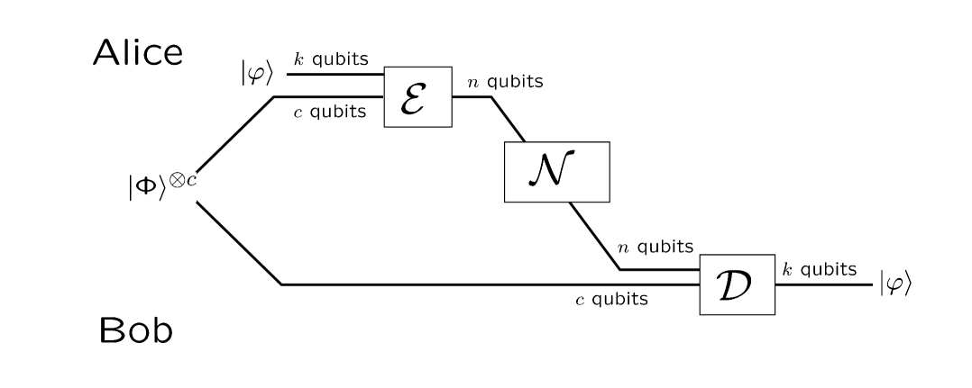
Figure 2: A generic entanglement assisted quantum code.

It is well known that for standard quantum error correction (i.e., that unassisted by entanglement) it suffices to consider errors from the Pauli group (see e.g. [28].) We will show this for entanglement-assisted quantum error correction. Denote by ${\cal L}$ the space of linear operators defined on the qubit Hilbert space ${\cal H}$. We will often encounter isometric operators $U:{\cal H}^{\otimes n_{1}}\rightarrow{\cal H}^{\otimes n_{2}}$. The corresponding superoperator, or completely positive, trace preserving (CPTP) map, is marked by a hat $\hat{U}:{\cal L}^{\otimes n_{1}}\rightarrow{\cal L}^{\otimes n_{2}}$ and defined by

$$\hat{U}(\rho)=U\rho U^{\dagger}.$$

Observe that $\hat{U}$ is independent of any phases factors multiplying $U$. Thus, for a Pauli operator $N_{\mathbf{u}}$, $\hat{N}_{\mathbf{u}}$ only depends on the equivalence class $[N_{\mathbf{u}}]$.

Our communication scenario involves two spatially separated parties, Alice and Bob, as depicted in Figure 2. The resources at their disposal are

• a noisy channel defined by a CPTP map ${\cal N}:{\cal L}^{\otimes n}\rightarrow{\cal L}^{\otimes n}$ taking density operators on Alice’s system to density operators on Bob’s system;

• the $c$ ebit state $|\Phi\rangle^{\otimes c}$ shared between Alice and Bob.

Alice wishes to send $k$ qubits perfectly to Bob using the above resources. An $[[n,k;c]]$ entanglement-assisted quantum error correcting (EAQEC) code consists of

• An encoding isometry ${\cal E}=\hat{U}_{\rm enc}:{\cal L}^{\otimes k}\otimes{\cal L}^{\otimes c}\rightarrow{\cal L}^{\otimes n}$

• A decoding CPTP map ${\cal D}:{\cal L}^{\otimes n}\otimes{\cal L}^{\otimes c}\rightarrow{\cal L}^{\otimes k}$

such that

$${\cal D}\circ{\cal N}\circ\hat{U}_{\rm enc}\circ\hat{U}_{\rm app}=\operatorname{id}^{\otimes k},$$

where ${U}_{\rm app}$ is the isometry which appends the state $|\Phi\rangle^{\otimes c}$,

$$U_{\rm app}|\varphi\rangle=|\varphi\rangle|\Phi\rangle^{\otimes c},$$

and $\operatorname{id}:{\cal L}\rightarrow{\cal L}$ is the identity map on a single qubit. The protocol thus uses up $c$ ebits of entanglement and generates $k$ perfect qubit channels. We represent it by the resource inequality (with a slight abuse of notation [12])

$$\langle{\cal N}\rangle+c\,[q\,q]\geq k\,[q\rightarrow q].$$

Even though a qubit channel is a strictly stronger resource than its static analogue, an ebit of entanglement, the parameter $k-c$ is still a good (albeit pessimistic) measure of the net noiseless quantum resources gained. It should be borne in mind that a negative value of $k-c$ still refers to a non-trivial protocol.

To make contact with classical error correction it is necessary to discretize the errors. This is done in two steps. First, the CPTP map ${\cal N}$ may be (non-uniquely) written in terms of its Kraus representation

$${\cal N}(\rho)=\sum_{i}A_{i}\rho A_{i}^{\dagger}.$$

Second, each $A_{i}$ may be expanded in the Pauli operators

$$A_{i}=\sum_{{\mathbf{u}}\in(\mathbb{Z}_{2})^{2n}}\alpha_{i,{\mathbf{u}}}N_{\mathbf{u}}.$$

Define the support of ${\cal N}$ by ${\rm supp}({\cal N})=\{{\mathbf{u}}\in(\mathbb{Z}_{2})^{2n}:\exists i,\alpha_{i,{\mathbf{u}}}\neq 0\}$. The following theorem allows us, absorbing ${U}_{\rm app}$ into ${U}_{\rm enc}$, to replace the continuous map ${\cal N}$ by the error set $S={\rm supp}({\cal N})$.

Theorem 2.1

If ${\cal D}\circ\hat{N}_{\mathbf{u}}\circ\hat{U}_{\rm enc}=\operatorname{id}^{\otimes k}$ for all ${\mathbf{u}}\in{\rm supp}({\cal N})$, then ${\cal D}\circ{\cal N}\circ\hat{U}_{\rm enc}=\operatorname{id}^{\otimes k}$.

Proof  We may extend the map ${\cal D}$ to its Stinespring dilation – an isometric map $\hat{U}_{\rm dec}$ with a larger target Hilbert space ${\cal L}^{\otimes k}\otimes{\cal L}^{\prime}$, such that

$${\cal D}=\operatorname{Tr}_{{\cal L}^{\prime}}\circ\hat{U}_{\rm dec}.$$

The premise of the theorem is equivalent to saying that for all ${\mathbf{u}}\in{\rm supp}({\cal N})$ and all pure states $|\varphi\rangle$ in ${\cal H}^{\otimes n}$,

$$U_{\rm dec}N_{\mathbf{u}}{U}_{\rm enc}|\varphi\rangle=|\varphi\rangle\otimes|{\mathbf{u}}\rangle$$

for some pure state $|{\mathbf{u}}\rangle\!\langle{\mathbf{u}}|$ on ${\cal L}^{\prime}$. By linearity

$$U_{\rm dec}A_{i}{U}_{\rm enc}|\varphi\rangle=|\varphi\rangle\otimes|i\rangle,$$

with the unnormalized state $|i\rangle=\sum_{\mathbf{u}}\alpha_{i,{\mathbf{u}}}|{\mathbf{u}}\rangle$. Furthermore,

$$\begin{split}(\hat{U}_{\rm dec}\circ{\cal N}\circ\hat{U}_{\rm enc})(|\varphi\rangle\!\langle\varphi|)&=U_{\rm dec}\left(\sum_{i}A_{i}{U}_{\rm enc}|\varphi\rangle\!\langle\varphi|{U}_{\rm enc}^{\dagger}A_{i}^{\dagger}\right)U_{\rm dec}^{\dagger}\\ &=|\varphi\rangle\!\langle\varphi|\otimes\sum_{i}|i\rangle\!\langle i|,\end{split}$$ (19)

where the second subsystem corresponds to ${\cal L}^{\prime}$. Tracing out the latter gives

$$({\cal D}\circ{\cal N}\circ\hat{U}_{\rm enc})(|\varphi\rangle\!\langle\varphi|)=|\varphi\rangle\!\langle\varphi|,$$

concluding the proof. $\Box$

2.2 The canonical error set and syndrome coding

By the results of the previous subsection, we are now interested in EAQEC codes which correct a particular error set $S\subset(\mathbb{Z}_{2})^{2n}$. We first restrict attention to a simple error set, which will turn out to be generic due to the results of Section 1.3.

Consider the following trivial encoding operation $\hat{U}_{0}$ defined by

$$U_{0}:|\varphi\rangle|\Phi\rangle^{\otimes c}\mapsto|\varphi\rangle|{\mathbf{0}}\rangle|\Phi\rangle^{\otimes c}.$$ (20)

In other words, the register containing $|{\mathbf{0}}\rangle$ (of size $\ell=n-k-c$ qubits) is appended to the registers containing $|\varphi\rangle$ (of size $k$ qubits) and $|\Phi\rangle^{\otimes c}$ (of size $c$ qubits each for Alice and Bob). What errors can she correct with such a simple-minded encoding?

Proposition 2.2

The code given by $U_{0}$ and a suitably defined decoding map ${\cal D}_{0}$ can correct the error set

$$S_{0}=\{\left({\mathbf{\alpha}}({\mathbf{a}},{\mathbf{a}}_{1},{\mathbf{a}}_{2}),{\mathbf{b}},{\mathbf{a}}_{2}|{\mathbf{\beta}}({\mathbf{a}},{\mathbf{a}}_{1},{\mathbf{a}}_{2}),{\mathbf{a}},{\mathbf{a}}_{1}\right):{\mathbf{b}},{\mathbf{a}}\in(\mathbb{Z}_{2})^{\ell},{\mathbf{a}}_{1},{\mathbf{a}}_{2}\in(\mathbb{Z}_{2})^{c}\},$$ (21)

for any functions ${\mathbf{\alpha}},{\mathbf{\beta}}:(\mathbb{Z}_{2})^{\ell}\times(\mathbb{Z}_{2})^{c}\times(\mathbb{Z}_{2})^{c}\rightarrow(\mathbb{Z}_{2})^{k}$.

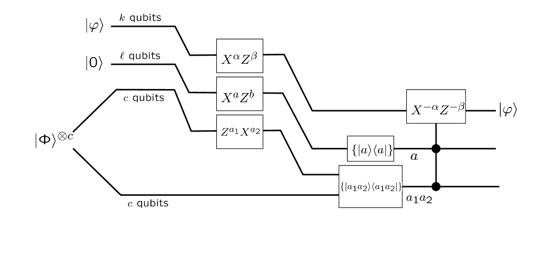
Figure 3: The canonical code.

Proof  The protocol is shown in figure 3. After applying an error $N_{\mathbf{u}}$ with

$${\mathbf{u}}=({\mathbf{\alpha}}({\mathbf{a}},{\mathbf{a}}_{1},{\mathbf{a}}_{2}),{\mathbf{b}},{\mathbf{a}}_{2}|{\mathbf{\beta}}({\mathbf{a}},{\mathbf{a}}_{1},{\mathbf{a}}_{2}),{\mathbf{a}},{\mathbf{a}}_{1}),$$ (22)

the encoded state $|\varphi\rangle|{\mathbf{0}}\rangle|\Phi\rangle^{\otimes c}$ becomes (up to a phase factor)

$$\begin{split}&Z^{{\mathbf{\alpha}}({\mathbf{a}},{\mathbf{a}}_{1},{\mathbf{a}}_{2})}X^{{\mathbf{\beta}}({\mathbf{a}},{\mathbf{a}}_{1},{\mathbf{a}}_{2})}|\varphi\rangle\otimes X^{{\mathbf{a}}}Z^{\mathbf{b}}|{\mathbf{0}}\rangle\otimes(Z^{{\mathbf{a}}_{1}}X^{{\mathbf{a}}_{2}}\otimes I)|\Phi\rangle^{\otimes c}\\ &=Z^{{\mathbf{\alpha}}({\mathbf{a}},{\mathbf{a}}_{1},{\mathbf{a}}_{2})}X^{{\mathbf{\beta}}({\mathbf{a}},{\mathbf{a}}_{1},{\mathbf{a}}_{2})}|\varphi\rangle\otimes|{\mathbf{a}}\rangle\otimes|{\mathbf{a}}_{1},{\mathbf{a}}_{2}\rangle,\end{split}$$ (23)

where $|{\mathbf{a}}\rangle=X^{{\mathbf{a}}}|{\mathbf{0}}\rangle$ and $|{\mathbf{a}}_{1},{\mathbf{a}}_{2}\rangle=(Z^{{\mathbf{a}}_{1}}X^{{\mathbf{a}}_{2}}\otimes I)|\Phi\rangle^{\otimes c}$. As the vector $({\mathbf{a}},{\mathbf{a}}_{1},{\mathbf{a}}_{2},{\mathbf{b}})^{{T}}$ completely specifies the error ${\mathbf{u}}$, it is called the error syndrome. The state (23) only depends on the reduced syndrome ${\bf r}=({\mathbf{a}},{\mathbf{a}}_{1},{\mathbf{a}}_{2})^{{T}}$. In effect, ${\mathbf{a}}$ and $({\mathbf{a}}_{1},{\mathbf{a}}_{2})$ have been encoded using plain and superdense coding, respectively. Bob, who holds the entire state (23), may identify the reduced syndrome using the results of section 1.4. Bob simultaneous measures the $Z^{{\mathbf{e}}_{1}},\dots,Z^{{\mathbf{e}}_{m}}$ observables to decode ${\mathbf{a}}$, the $Z^{{\mathbf{e}}_{1}}\otimes Z^{{\mathbf{e}}_{1}},\dots,Z^{{\mathbf{e}}_{m}}\otimes Z^{{\mathbf{e}}_{m}}$ observables to decode ${\mathbf{a}}_{1}$, and the $X^{{\mathbf{e}}_{1}}\otimes X^{{\mathbf{e}}_{1}},\dots,X^{{\mathbf{e}}_{m}}\otimes X^{{\mathbf{e}}_{m}}$ observables to decode ${\mathbf{a}}_{2}$. He then performs $Z^{-{\mathbf{\alpha}}({\mathbf{a}},{\mathbf{a}}_{1},{\mathbf{a}}_{2})}X^{-{\mathbf{\beta}}({\mathbf{a}},{\mathbf{a}}_{1},{\mathbf{a}}_{2})}$ on the remaining $k$ qubit system, leaving it in the state $|\varphi\rangle$.

Since the goal is the transmission of quantum information, no actual measurement is necessary. Instead, Bob can perform the CPTP map ${\cal D}_{0}$ consisting of the controlled unitary

$$U_{0\,\rm{dec}}=\sum_{{\mathbf{a}},{\mathbf{a}}_{1},{\mathbf{a}}_{2}}Z^{-{\mathbf{\alpha}}({\mathbf{a}},{\mathbf{a}}_{1},{\mathbf{a}}_{2})}X^{-{\mathbf{\beta}}({\mathbf{a}},{\mathbf{a}}_{1},{\mathbf{a}}_{2})}\otimes|{\mathbf{a}}\rangle\!\langle{\mathbf{a}}|\otimes|{\mathbf{a}}_{1},{\mathbf{a}}_{2}\rangle\!\langle{\mathbf{a}}_{1},{\mathbf{a}}_{2}|,$$

followed by discarding the last two subsystems. $\Box$

The above code is degenerate with respect to the error set $S$, which means that the error can be corrected without knowing the full error syndrome.

We can characterize our code in terms of the parity check matrix $F$ given by

$$F=\left(\begin{array}[]{c}F_{I}\\ F_{S}\end{array}\right),$$ (24)

$$F_{I}=\left(\begin{array}[]{ccc|ccc}{\mathbf{0}}_{\ell\times k}&{\mathbf{I}}_{\ell\times\ell}&{\mathbf{0}}_{\ell\times c}&{\mathbf{0}}_{\ell\times k}&{\mathbf{0}}_{\ell\times\ell}&{\mathbf{0}}_{\ell\times c}\end{array}\right),$$ (25)

$$F_{S}=\left(\begin{array}[]{ccc|ccc}{\mathbf{0}}_{c\times k}&{\mathbf{0}}_{c\times\ell}&{\mathbf{I}}_{c\times c}&{\mathbf{0}}_{c\times k}&{\mathbf{0}}_{c\times\ell}&{\mathbf{0}}_{c\times c}\\ {\mathbf{0}}_{c\times k}&{\mathbf{0}}_{c\times\ell}&{\mathbf{0}}_{c\times c}&{\mathbf{0}}_{c\times k}&{\mathbf{0}}_{c\times\ell}&{\mathbf{I}}_{c\times c}\end{array}\right),$$ (26)

with $\ell=n-k-c$.

The vector space ${\rm rowspace}(F)$ decomposes into a direct sum of the isotropic subspace ${\rm rowspace}(F_{I})$ and symplectic subspace ${\rm rowspace}(F_{S})$, as in Theorem 1.1. Define the symplectic code corresponding to $F$ by

$$C_{0}={\rm rowspace}(F)^{\perp}$$

where

$$V^{\perp}=\{{\mathbf{w}}:{\mathbf{w}}\odot{\mathbf{u}}^{{T}}=0,\,\,\forall{\mathbf{u}}\in V\}.$$

Note that $(V^{\perp})^{\perp}=V$. Then $C_{0}^{\perp}={\rm rowspace}(F)$, ${\rm iso}(C_{0}^{\perp})={\rm rowspace}(F_{I})$ and ${\rm symp}(C_{0}^{\perp})={\rm rowspace}(F_{S})$.

The number of ebits used in the code is

$$c=\frac{1}{2}\dim{\rm rowspace}(F_{S})$$

and the number of encoded qubits is

$$k=n-\dim{\rm rowspace}(F_{I})-{\small\frac{1}{2}}\dim{\rm rowspace}(F_{S}).$$

The parameter $k-c$ which is the number of encoded qubits minus the number of ebits used is independent of the symplectic structure of $F$:

$${k}-c=n-\dim{\rm rowspace}(F).$$

The error set $S_{0}$ can be described in terms of $F$:

Proposition 2.3

The set $S_{0}$ of errors correctable by the code ${\cal E}_{0}$ is such that, if ${\mathbf{u}},{\mathbf{u}}^{\prime}\in S_{0}$ and ${\mathbf{u}}\neq{\mathbf{u}}^{\prime}$, then either

1. ${\mathbf{u}}-{\mathbf{u}}^{\prime}\not\in C_{0}$ (equivalently: $F\odot({\mathbf{u}}-{\mathbf{u}}^{\prime})^{{T}}\neq{\mathbf{0}}^{{T}}$), or

2. ${\mathbf{u}}-{\mathbf{u}}^{\prime}\in{\rm iso}(C_{0}^{\perp})$ (equivalently: ${\mathbf{u}}-{\mathbf{u}}^{\prime}\in{\rm rowspace}(F_{I})$)

Proof  If ${\mathbf{u}}$ is given by (22) then $F\odot{\mathbf{u}}^{{T}}={\bf r}=({\mathbf{a}},{\mathbf{a}}_{1},{\mathbf{a}}_{2})^{{T}}$, the reduced error syndrome. By definition (21), two distinct elements of $S_{0}$ either have different reduced syndromes $({\mathbf{a}},{\mathbf{a}}_{1},{\mathbf{a}}_{2})$ (condition 1) or they differ by a vector of the form $({\mathbf{0}},{\mathbf{b}},{\mathbf{0}}|{\mathbf{0}},{\mathbf{0}},{\mathbf{0}})$ (condition 2). Observe that condition 1 is analogous to the usual error correcting condition for classical codes [27]. $\Box$

The parity check matrix $F$ also specifies the encoding and decoding operations. The space ${\cal H}^{\otimes k}$ is encoded into the codespace defined by

$${\cal C}_{0}=\{U_{0}|\varphi\rangle|\Phi\rangle^{\otimes c}:|\varphi\rangle\in{\cal H}^{\otimes k}\}.$$

It is not hard to see that the codespace is the simultaneous $+1$ eigenspace of the commuting operators:

1. $I\otimes Z^{{\mathbf{e}}_{i}}\otimes I\otimes I,\,\,i=1,\dots,\ell$;

2. $I\otimes I\otimes Z^{{\mathbf{e}}_{j}}\otimes Z^{{\mathbf{e}}_{j}},\,\,j=1,\dots,c$;

3. $I\otimes I\otimes X^{{\mathbf{e}}_{j}}\otimes X^{{\mathbf{e}}_{j}},\,\,j=1,\dots,c$.

Above, the first three operators act on Alice’s qubits and the fourth on Bob’s. Define the matrix

$$B=\left(\begin{array}[]{c|c}{\mathbf{0}}_{\ell\times c}&{\mathbf{0}}_{\ell\times c}\\ {\mathbf{I}}_{c\times c}&{\mathbf{0}}_{c\times c}\\ {\mathbf{0}}_{c\times c}&{\mathbf{I}}_{c\times c}\end{array}\right).$$ (27)

Define the augmented parity check matrix

$$F_{\rm aug}=(F,B)=\left(\begin{array}[]{cccc|cccc}{\mathbf{0}}_{\ell\times k}&{\mathbf{I}}_{\ell\times\ell}&{\mathbf{0}}_{\ell\times c}&{\mathbf{0}}_{\ell\times c}&{\mathbf{0}}_{\ell\times k}&{\mathbf{0}}_{\ell\times\ell}&{\mathbf{0}}_{\ell\times c}&{\mathbf{0}}_{\ell\times c}\\ {\mathbf{0}}_{c\times k}&{\mathbf{0}}_{c\times\ell}&{\mathbf{I}}_{c\times c}&{\mathbf{I}}_{c\times c}&{\mathbf{0}}_{c\times k}&{\mathbf{0}}_{c\times\ell}&{\mathbf{0}}_{c\times c}&{\mathbf{0}}_{c\times c}\\ {\mathbf{0}}_{c\times k}&{\mathbf{0}}_{c\times\ell}&{\mathbf{0}}_{c\times c}&{\mathbf{0}}_{c\times c}&{\mathbf{0}}_{c\times k}&{\mathbf{0}}_{c\times\ell}&{\mathbf{I}}_{c\times c}&{\mathbf{I}}_{c\times c}\end{array}\right).$$ (28)

Observe that ${\rm rowspace}(F_{\rm aug})$ is purely isotropic. The codespace is now described as the simultaneous $+1$ eigenspace of

$$\{N_{\mathbf{w}}:{\mathbf{w}}\in{\rm rowspace}(F_{\rm aug})\},$$

or, equivalently that of

$${\cal G}_{0}=\{N_{\mathbf{w}}:{\mathbf{w}}{\rm\,\,is\,\,a\,\,row\,\,of\,\,}F_{\rm aug}\}.$$

The decoding operation ${\cal D}_{0}$ is also described in terms of $F$. The reduced syndrome ${\bf r}=F\odot{\mathbf{u}}^{{T}}$ is obtained by simultaneously measuring the observables in ${\cal G}_{0}$. The reduced error syndrome corresponds to a number of possible errors ${\mathbf{u}}\in S_{0}$ which all have an identical effect on the codespace. Bob performs $\hat{N}_{{\mathbf{u}}}=\hat{N}_{-{\mathbf{u}}}$ to undo the error.

2.3 The general case

We now present our main result: how to convert an arbitrary $(n+\hat{k})$-dimensional subspace $C$ of $(\mathbb{Z}_{2})^{2n}$ into a EAQEC code. Consider the $(n-\hat{k})$-dimensional subspace $C^{\perp}$. By Theorem 1.1, there exists a symplectic basis of $(\mathbb{Z}_{2})^{2n}$ consisting of hyperbolic pairs $({\mathbf{u}}_{i},{\mathbf{v}}_{i})$, $i=1,\dots,n$, such that the ordered set ${\cal R}=\{{\mathbf{u}}_{k+1},\dots,{\mathbf{u}}_{n},{\mathbf{v}}_{k+\ell+1},\dots,{\mathbf{v}}_{n}\}$ is a basis for $C^{\perp}$, for some $c,\ell\geq 0$ with $2c+\ell=n-\hat{k}$, and $k-c=\hat{k}$. Let $H$ be the matrix whose rows consist of the elements of ${\cal R}$ in the order given from top to bottom. Let $\Upsilon$ be the symplectomorphism defined by

$$\Upsilon({\mathbf{u}}_{i}) = {\mathbf{g}}_{i}$$ (29)

$$\Upsilon({\mathbf{v}}_{i}) = {\mathbf{h}}_{i}.$$ (30)

Recall the matrix $F$ given by (24)-(26). Observe that, with a slight abuse of notation,

$$\Upsilon(H)=F$$

in the sense that $\Upsilon$ takes the $i$th row of $H$ to the $i$th row of $F$. We may extend $\Upsilon$ to act on $(\mathbb{Z}_{2})^{2(n+c)}$, including a trivial action on the bits corresponding to Bob’s side. Then

$$\Upsilon(H_{\rm aug})=F_{\rm aug},$$ (31)

where $H_{\rm aug}=(H,B)$.

In terms of vector spaces

$$\Upsilon(C^{\perp}) = C_{0}^{\perp},$$ (32)

$$\Upsilon({\rm iso}(C^{\perp})) = {\rm iso}(C_{0}^{\perp}).$$ (33)

Note that $c=\frac{1}{2}\dim{\rm symp}(C^{\perp})$. We our now ready for our main result:

Theorem 2.4

There exists an $[[n,k;c]]$ EAQEC code $(\hat{U}_{\rm enc},{\cal D})$ with the following properties:

1. It can correct the error set $S$ defined by: if ${\mathbf{u}},{\mathbf{u}}^{\prime}\in S$ and ${\mathbf{u}}\neq{\mathbf{u}}^{\prime}$, then either

   1. ${\mathbf{u}}-{\mathbf{u}}^{\prime}\not\in C$ (equivalently: $H\odot({\mathbf{u}}-{\mathbf{u}}^{\prime})^{{T}}\neq{\mathbf{0}}^{{T}}$), or

   2. ${\mathbf{u}}-{\mathbf{u}}^{\prime}\in{\rm iso}(C^{\perp})$ (equivalently: ${\mathbf{u}}-{\mathbf{u}}^{\prime}\in{\rm rowspace}(H_{I})$).

2. The codespace ${\cal C}=\hat{U}_{\rm enc}({\cal H}^{\otimes k})$ is a simultaneous eigenspace of the ordered set

   $${\cal G}=\{N_{\mathbf{w}}:{\mathbf{w}}{\rm\,\,is\,\,a\,\,row\,\,of\,\,}H_{\rm aug}\},$$

   where $H_{\rm aug}=(H,B)$, with $B$ given by (27).

3. To decode, the reduced error syndrome

   $${\bf r}=H\odot{\mathbf{u}}^{{T}}$$ (34)

   is obtained by simultaneously measuring the observables from ${\cal G}$. Bob finds a ${\mathbf{u}}$ satisfying (34) and performs $\hat{N}_{{\mathbf{u}}}$ to undo the error.

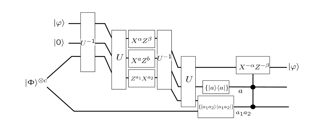
Figure 4: Generalizing the canonical code construction.

Remark   The above theorem generalizes the error correcting conditions of [17, 8] for quantum error correcting codes unassisted by entanglement. When $c=0$ then $C^{\perp}={\rm iso}(C^{\perp})$ and no entanglement is used in the protocol. We call such codes dual-containing.

Proof  By Theorem 1.2 there exists a unitary $U_{\Upsilon}$ such that for all ${\mathbf{u}}\in(\mathbb{Z}_{2})^{2n}$

$$[N_{\Upsilon({\mathbf{u}})}]=[U_{\Upsilon}N_{{\mathbf{u}}}U_{\Upsilon}^{-1}],$$ (35)

and hence

$$\hat{N}_{\Upsilon({\mathbf{u}})}=\hat{U}_{\Upsilon}\circ\hat{N}_{{\mathbf{u}}}\circ\hat{U}_{\Upsilon}^{-1}.$$

The above also holds for $\Upsilon$ and $\hat{U}_{\Upsilon}$ extended to act trivially on Bob’s side.

Our EAQEC code is defined by $U_{\rm enc}=U_{\Upsilon}^{-1}U_{0}$ and ${\cal D}={\cal D}_{0}\circ\hat{U}_{\Upsilon}$, as shown in Figure 4.

1. Recall the error set $S_{0}$ defined in Proposition 2.3. From (32) and (33) it follows that $\Upsilon(S)=S_{0}$. By Proposition 2.3, for all ${\mathbf{u}}\in S$,

   $${\cal D}_{0}\circ\hat{N}_{\Upsilon({\mathbf{u}})}\circ\hat{U}_{0}=\operatorname{id}^{\otimes k},$$

   from which

   $${\cal D}\circ\hat{N}_{{\mathbf{u}}}\circ\hat{U}_{\rm enc}=\operatorname{id}^{\otimes k}$$

   follows. Thus, the code $(\hat{U}_{\rm enc},{\cal D})$ corrects the error set $S$.

2. The codespace is ${\cal C}=U_{\Upsilon}^{-1}({\cal C}_{0})$, by definition. According to (31), ${\cal C}_{0}$ is the simultaneous $+1$ eigenspace of

   $${\cal G}_{0}=\{N_{\Upsilon({\mathbf{w}})}:{\mathbf{w}}{\rm\,\,is\,\,a\,\,row\,\,of\,\,}H_{\rm aug}\},$$

   or by (35), the set

   $${\cal G}^{\prime}_{0}=\{U_{\Upsilon}N_{{\mathbf{w}}}U_{\Upsilon}^{-1}:{\mathbf{w}}{\rm\,\,is\,\,a\,\,row\,\,of\,\,}H_{\rm aug}\}.$$

   Lemma 2.5 now implies that the codespace ${\cal C}$ is a simultaneous eigenspace of ${\cal G}$.

3. Assume that error ${\mathbf{u}}\in S$ occurs. The operation ${\cal D}_{0}$ involves

   1. measuring the set of operators given by ${\cal G}_{0}$, or equivalently ${\cal G}^{\prime}_{0}$, yielding the reduced syndrome

      $${\bf r}=F\odot\Upsilon({\mathbf{u}})^{{T}};$$

   2. performing $\hat{N}_{\Upsilon({\mathbf{u}})}$, where $\Upsilon({\mathbf{u}})\in S_{0}$ is an error consistent with the observed syndrome ${\bf r}$.

   (34) holds because

   $${\bf r}=\Upsilon(H)\odot\Upsilon({\mathbf{u}})^{{T}}=H\odot{\mathbf{u}}^{{T}}.$$

   By lemma 2.6, performing ${\cal D}={\cal D}_{0}\circ\hat{U}_{\Upsilon}$ is equivalent to measuring the set ${\cal G}$, followed by performing $\hat{N}_{\mathbf{u}}=\hat{U}^{-1}_{\Upsilon}\circ\hat{N}_{\Upsilon({\mathbf{u}})}\circ\hat{U}_{\Upsilon}$, followed by $\hat{U}_{\Upsilon}$ to undo the encoding. If the final $\hat{U}_{\Upsilon}$ is omitted, one recovers the encoded state rather than the original one.

$\Box$

Lemma 2.5

If ${\cal C}_{0}$ is a simultaneous eigenspace of Pauli operators from the set ${\cal G}^{\prime}_{0}$ then ${\cal C}=U^{-1}({\cal C}_{0})$ is a simultaneous eigenspace of Pauli operators from the set ${\cal G}=\{U^{-1}{\mathbf{A}}U:{\mathbf{A}}\in{\cal G}^{\prime}_{0}\}$.

Proof  Observe that if

$${\mathbf{A}}|\psi\rangle=\alpha|\psi\rangle,$$

then

$$(U^{-1}{\mathbf{A}}U)U^{-1}|\psi\rangle=\alpha U^{-1}|\psi\rangle.$$

$\Box$

Lemma 2.6

Performing $U$ followed by measuring the operator ${\bf A}$ is equivalent to measuring the operator $U^{-1}{\bf A}U$ followed by performing $U$.

Proof  Let $\Pi_{i}$ be a projector onto the eigenspace corresponding to eigenvalue $\lambda_{i}$ of ${\bf A}$. Performing $U$ followed by measuring the operator ${\bf A}$ is equivalent to the instrument (generalized measurement) given by the set of operators $\{\Pi_{i}U\}$. The operator $U^{-1}{\bf A}U$ has the same eigenvalues as $\bf A$, and the projector onto the eigenspace corresponding to eigenvalue $\lambda_{i}$ is $U^{-1}\Pi_{i}U$. Measuring the operator $U^{-1}{\bf A}U$ followed by performing $U$ is equivalent to the instrument $\{U(U^{-1}\Pi_{i}U)\}=\{\Pi_{i}U\}$. $\Box$

2.4 Distance

The notion of distance provides a convenient way to characterize the error correcting properties of a code. We start by defining the weight of a vector ${\mathbf{u}}=({\mathbf{z}}|{\mathbf{x}})\in(\mathbb{Z}_{2})^{2n}$ by $\operatorname{wt}({\mathbf{u}})=\operatorname{wt}({\mathbf{z}}\vee{\mathbf{x}})$. Here $\vee$ denotes the bitwise logical “or”, and $\operatorname{wt}({\mathbf{y}})$ is the number of non-zero bits in ${\mathbf{y}}\in(\mathbb{Z}_{2})^{n}$. In terms of the Pauli group, $\operatorname{wt}({\mathbf{u}})$ is the number of single qubit Pauli matrices in $N_{\mathbf{u}}$ not equal to the identity $I$.

Consider a symplectic code $C$. The distance of $C$ is the maximum $d$ such that for each nonzero ${\mathbf{u}}$ of weight $<d$ either

1. ${\mathbf{u}}\not\in C$, or

2. ${\mathbf{u}}\in{\rm iso}(C^{\perp})$

It is called non-degenerate if the second condition is not invoked. A code is said to correct $t$ errors if it corrects the error set $\{{\mathbf{u}}:\operatorname{wt}({\mathbf{u}})\leq t\}$ but not $\{{\mathbf{u}}:\operatorname{wt}({\mathbf{u}})\leq t+1\}$. Comparing these definitions with Theorem 2.4, a code with distance $d=2t+1$ can correct $t$ errors. An $[[n,k;c]]$ EAQEC code with distance $d$ will be referred to as an $[[n,k,d;c]]$ code.

3 Relation to quaternary codes

We shall now show how to construct non-degenerate EAQEC codes from classical codes over $\mathbb{F}_{4}$, generalizing the work of [8]. Following the presentation of Forney et al. [20], the addition table of the additive group of the quaternary field $\mathbb{F}_{4}=\{0,1,\omega,\overline{\omega}\}$ is given by

$$\begin{array}[]{|c|cccc|}\hline\cr+&0&\overline{\omega}&1&\omega\\ \hline\cr 0&0&\overline{\omega}&1&{\omega}\\ \overline{\omega}&\overline{\omega}&0&\omega&1\\ 1&1&{\omega}&0&\overline{\omega}\\ {\omega}&\omega&1&\overline{\omega}&0\\ \hline\cr\end{array}$$

Comparing the above to the addition table of $(\mathbb{Z}_{2})^{2}$ establishes the isomorphism $\gamma:\mathbb{F}_{4}\rightarrow(\mathbb{Z}_{2})^{2}$, given by the table

$$\begin{array}[]{|c|c|}\hline\cr\mathbb{F}_{4}&(\mathbb{Z}_{2})^{2}\\ \hline\cr 0&00\\ \overline{\omega}&01\\ 1&11\\ \omega&10\\ \hline\cr\end{array}$$

The multiplication table for $\mathbb{F}_{4}$ is defined as

$$\begin{array}[]{|c|cccc|}\hline\cr\times&0&\overline{\omega}&1&\omega\\ \hline\cr 0&0&0&0&0\\ \overline{\omega}&0&\omega&\overline{\omega}&1\\ 1&0&\overline{\omega}&1&\omega\\ \omega&0&1&\omega&\overline{\omega}\\ \hline\cr\end{array}$$

Define the traces ($\operatorname{Tr}$) of the elements $\{0,1,\omega,\overline{\omega}\}$ of $\mathbb{F}_{4}$ as $\{0,0,1,1\}$, and their conjugates (“^†”) as $\{0,1,\overline{\omega},\omega\}$. Intuitively, $\operatorname{Tr}a$ measures the “$\omega$-ness” of $a\in\mathbb{F}_{4}$. Observe that $a=0$ if and only if both $\operatorname{Tr}\omega a=0$ and $\operatorname{Tr}\overline{\omega}a=0$. The Hermitian inner product of two elements $a,b\in\mathbb{F}_{4}$ is defined as $\langle{a},{b}\rangle=a^{\dagger}b\in\mathbb{F}_{4}$. The trace product is defined as $\operatorname{Tr}\langle{a},{b}\rangle\in\mathbb{F}_{2}$. The trace product table is readily found to be

$$\begin{array}[]{|c|cccc|}\hline\cr\operatorname{Tr}\langle{\,},{}\rangle&0&\overline{\omega}&1&\omega\\ \hline\cr 0&0&0&0&0\\ \overline{\omega}&0&0&1&1\\ 1&0&1&0&1\\ \omega&0&1&1&0\\ \hline\cr\end{array}$$

Comparing the above to the $\odot$ table of $(\mathbb{Z}_{2})^{2}$ establishes the identity

$$\operatorname{Tr}\langle{a},{b}\rangle={\gamma(a)\odot\gamma(b)}.$$

These notions can be generalized to $n$-dimensional vector spaces over $\mathbb{F}_{4}$. Thus, for ${\mathbf{a}},{\mathbf{b}}\in(\mathbb{F}_{4})^{n}$,

$$\operatorname{Tr}\langle{{\mathbf{a}}},{{\mathbf{b}}}\rangle={\gamma({\mathbf{a}})\odot\gamma({\mathbf{b}})^{{T}}}.$$ (36)

Let $\operatorname{wt}_{4}({\mathbf{a}})$ be the number of non-zero bits in ${\mathbf{a}}\in(\mathbb{F}_{4})^{n}$. Then we have another identity

$$\operatorname{wt}(\gamma({\mathbf{a}}))=\operatorname{wt}_{4}({\mathbf{a}}),$$ (37)

where $\gamma({\mathbf{a}})\in(\mathbb{Z}_{2})^{2n}$.

Proposition 3.1

If a classical $[n,k,d]_{4}$ code exists then an $[[n,2k-n+c,d;c]]$ EAQEC code exists for some non-negative integer $c$.

Proof  Consider a classical $[n,k,d]_{4}$ code (the subscript $4$ emphasizes that the code is over $\mathbb{F}_{4}$) with an $(n-k)\times n$ quaternary parity check matrix $H_{4}$. By definition, for each nonzero ${\mathbf{a}}\in(\mathbb{F}_{4})^{n}$ such that $\operatorname{wt}_{4}({\mathbf{a}})<d$,

$$\langle{H_{4}},{{\mathbf{a}}}\rangle\neq{\mathbf{0}}^{{T}}.$$

This is equivalent to the logical statement

$$\operatorname{Tr}\langle{\omega H_{4}},{{\mathbf{a}}}\rangle\neq{\mathbf{0}}^{{T}}\,\,\vee\,\,\operatorname{Tr}\langle{\overline{\omega}H_{4}},{{\mathbf{a}}}\rangle\neq{\mathbf{0}}^{{T}}.$$

This is further equivalent to

$$\operatorname{Tr}\langle{\widetilde{H}_{4}},{{\mathbf{a}}}\rangle\neq{\mathbf{0}}^{{T}},$$

where

$$\widetilde{H}_{4}=\left(\begin{array}[]{c}\omega H_{4}\\ \overline{\omega}H_{4}\end{array}\right).$$ (38)

Define the $(2n-2k)\times 2n$ symplectic matrix $H=\gamma(\widetilde{H}_{4})$. By the correspondences (36) and (37),

$$H\odot{\mathbf{u}}^{{T}}\neq{\mathbf{0}}^{{T}},$$

holds for each nonzero ${\mathbf{u}}\in(\mathbb{Z}_{2})^{2n}$ with $\operatorname{wt}({\mathbf{u}})<d$. Thus $C={\rm rowspace}(H)^{\perp}$ defines a non-degenerate $[n,2k-n+c,d;c]$ EAQEC code, where

$$c=\frac{1}{2}\dim{\rm symp}(C).$$

$\Box$

Any classical binary $[n,k,d]_{2}$ code may be viewed as an quaternary $[n,k,d]_{4}$. In this case, the above construction gives rise to a CSS-type code.

4 Catalytic quantum error correcting codes

So far we have been considering communication scenarios involving two spatially separated parties Alice and Bob connected by a noisy channel ${\cal N}$. In this setting, entanglement between them is a meaningful resource. What if Alice and Bob are separated only in time? For example, ${\cal N}$ could represent the time evolution of the state of a quantum computer. Then entanglement between Alice and Bob does not make sense any more.

An alternative (in the communication picture) is to let Alice and Bob have access to a noiseless channel, rather than entanglement. This channel serves as a catalyst and is returned at the end of the protocol. An $[[n,k;c]]$ catalytic quantum error correcting (CQEC) code is defined by

• An encoding isometry ${\cal E}:{\cal L}^{\otimes k}\otimes{\cal L}^{\otimes c}\rightarrow{\cal L}^{\otimes n}$

• A decoding CPTP map ${\cal D}:{\cal L}^{\otimes n}\otimes{\cal L}^{\otimes c}\rightarrow{\cal L}^{\otimes k}$

such that

$${\cal D}\circ({\cal N}\otimes\operatorname{id}^{\otimes c})\circ{\cal E}=\operatorname{id}^{\otimes{k}}=\operatorname{id}^{\otimes k-c}\otimes\operatorname{id}^{\otimes c}.$$ (39)

The above may be written as a resource inequality

$$\langle{\cal N}\rangle+c\,[q\rightarrow q]\geq(k-c)\,[q\rightarrow q]+c\,[q\rightarrow q].$$ (40)

The net rate of the CQEC code is given by $(k-c)/n$. Figure 5 shows how any $[[n,{k};c]]$ EAQEC code $({\cal E},{\cal D})$ gives rise to a CQEC code with the same parameters. This construction may be understood in terms of resource inequalities. The simple protocol called entanglement distribution written as

$$c\,[q\rightarrow q]\geq c\,[q\,q],$$

creates $c$ ebits of entanglement by sending half of a locally prepared state $|\Phi\rangle^{\otimes c}$ through the channel $\operatorname{id}^{\otimes c}$. The CQEC code is obtained by combining entanglement distribution with the EAQEC code:

$$\begin{split}&\langle{\cal N}\rangle+c\,[q\rightarrow q]\\ &\geq\langle{\cal N}\rangle+c\,[q\,q]\\ &\geq k\,[q\rightarrow q]\\ &=(k-c)\,[q\rightarrow q]+c\,[q\rightarrow q].\end{split}$$ (41)

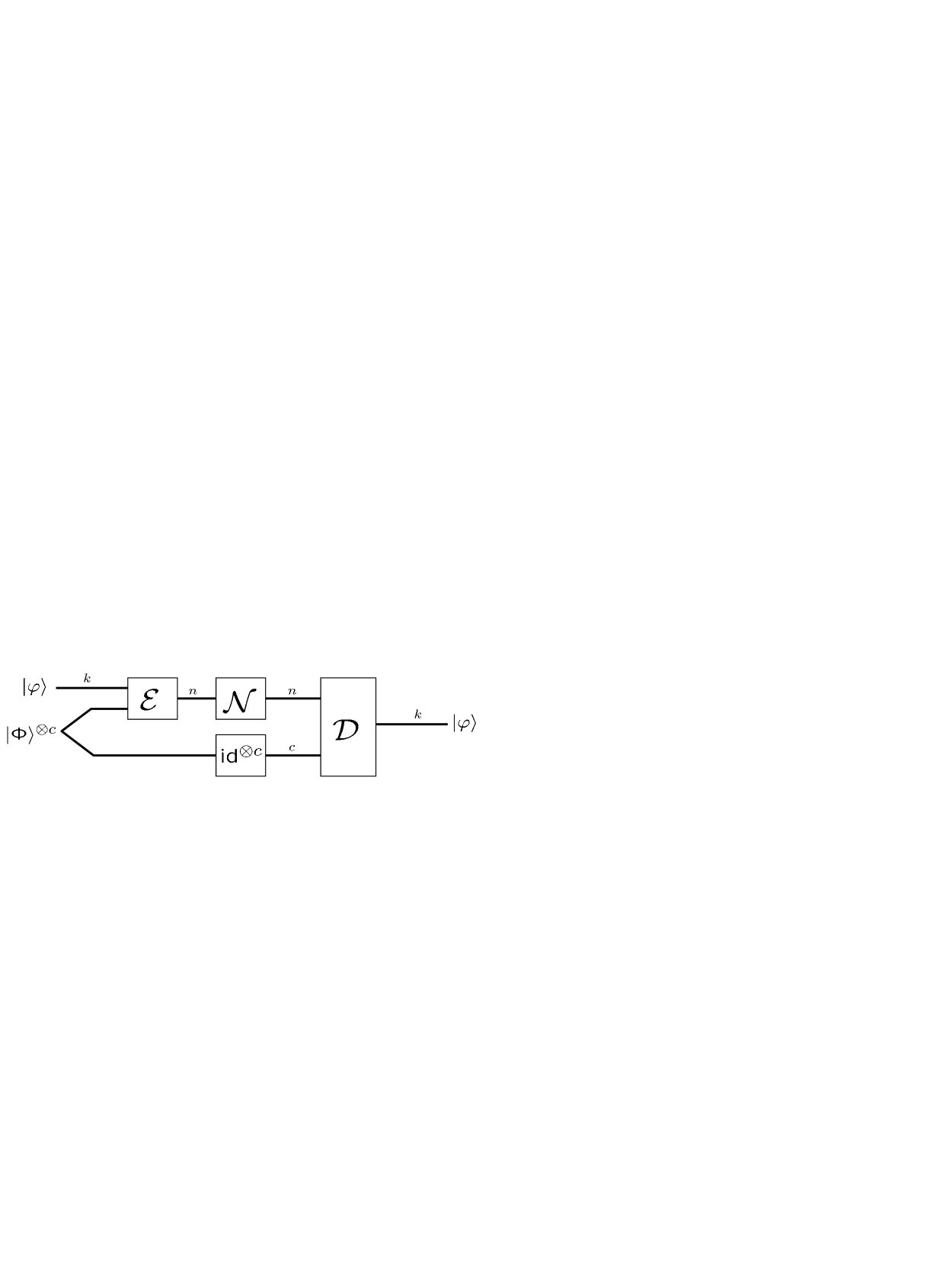
Figure 5: A catalytic quantum error-correcting code.

Assume now that Alice and Bob have access to $m$ copies of the chanel ${\cal N}$. Performing the CQEC protocol $m$ times in parallel (i.e. using the code $({\cal E}^{\otimes m},{\cal D}^{\otimes m})$) gives

$$m\langle{\cal N}\rangle+mc\,[q\rightarrow q]\geq m(k-c)\,[q\rightarrow q]+mc\,[q\rightarrow q].$$

The size of the catalyst can actually be reduced from $mc$ to $c$:

$$m\langle{\cal N}\rangle+c\,[q\rightarrow q]\geq m(k-c)\,[q\rightarrow q]+c\,[q\rightarrow q].$$ (42)

The proof is by induction. The statement is trivial for $m=1$. For the inductive step, assume true for $m$. Then (42) holds for $m+1$:

$$\begin{split}&(m+1)\langle{\cal N}\rangle+c\,[q\rightarrow q]\\ &=\langle{\cal N}\rangle+m\langle{\cal N}\rangle+c\,[q\rightarrow q]\\ &\geq\langle{\cal N}\rangle+m(k-c)\,[q\rightarrow q]+c\,[q\rightarrow q]\\ &\geq m(k-c)\,[q\rightarrow q]+(k-c)\,[q\rightarrow q]+c\,[q\rightarrow q].\end{split}$$ (43)

A more conventional formulation of this catalyst reduction is given in the lemma below.

Lemma 4.1

If (39) is satisfied then for any non-negative integer $m$ there exists a CQEC code $({\cal E}_{m},{\cal D}_{m})$ for the channel ${\cal N}^{\otimes m}$ in the sense that

$${\cal D}_{m}\circ({\cal N}^{\otimes m}\otimes\operatorname{id}^{\otimes c})\circ{\cal E}_{m}=\operatorname{id}^{\otimes m(k-c)}\otimes\operatorname{id}^{\otimes c}.$$

Proof  The inductive step is shown in the Figure 6. $\Box$

The above construction is rather sensitive to perturbations. If in any particular block a channel worse than ${\cal N}$ is experienced, the resulting channel will not be pure and the next block will start with an impure catalyst.

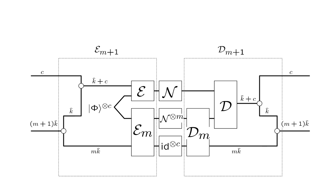
Figure 6: The inductive step.

One may rightly ask about where one could obtain a catalyst to begin with. A possibility is to use an ordinary $c=0$ QEC code. This is shown in Figure 7. An $[n,{k};c]$ CQEC code for the channel ${\cal N}$ combined with a $[n^{\prime},c;0]$ QEC code for the channel ${\cal N}^{\prime}$ gives an $[n+n^{\prime},{k};0]$ QEC code for the channel ${\cal N}\otimes{\cal N}^{\prime}$. The combined code can be used as a catalyst for an even larger code. In this way a sizeable catalyst can be built up pretty quickly.

It is worth looking at this construction from a purely mathematical point of view. Let $C\subset(\mathbb{Z}_{2})^{2n}$ and $C^{\prime}\subset(\mathbb{Z}_{2})^{2n^{\prime}}$ be the symplectic codes corresponding to the $[n,{k};c]$ CQEC code and $[n^{\prime},c;0]$ QEC code, respectively. Let $H$ and $H^{\prime}$ be the respective parity check matrices, as in section 2.3. Note that ${C^{\prime}}^{\perp}={\rm iso}({C^{\prime}}^{\perp})$. Let ${\mathbf{u}}_{i}$, $i=1,\dots,c$, be vectors in $(\mathbb{Z}_{2})^{2n^{\prime}}$ which, together with a basis for ${C^{\prime}}^{\perp}$, form a maximal $n^{\prime}$-dimensional isotropic subspace of $(\mathbb{Z}_{2})^{2n^{\prime}}$. Recall the notation ${\mathbf{g}}_{i}=({\mathbf{e}}_{i}|{\mathbf{0}})\in(\mathbb{Z}_{2})^{2c}$. Let $\Upsilon$ be a symplectomorphism such that $\Upsilon({\mathbf{g}}_{i})={\mathbf{u}}_{i}$. Define the $(n-{k}+c)\times 2n^{\prime}$ matrix $B^{\prime}=\Upsilon(B)$ with $B$ defined as in (27) and $\ell=n-{k}-c$. Note that the rows of $B^{\prime}$ are in $C^{\prime}$. Then

$$\widetilde{H}_{\rm aug}=\left(\begin{array}[]{cc}H,&B^{\prime}\\ {\mathbf{0}}_{(n^{\prime}-c)\times 2n},&H^{\prime}\end{array}\right)$$

is the parity check matrix for the combined $[n+n^{\prime},{k};0]$ QEC code. By construction, is must be dual-containing.

Figure 7: Constructing a QEC code from a seed QEC code and a CQEC code.

5 A variation on EAQEC codes

One lesson learned from quantum Shannon theory [13] is that catalytic and non-catalytic codes have similar performance. In this section we mimic the quantum Shannon theoretical construction from [13]. First we construct codes for sending classical information with entanglement assistance. Then we make these protocols coherent in the sense of [19, 13] to obtain a variation on EAQEC codes in which entanglement is generated as well as quantum communication. The end result is what we will call “type II” EAQEC codes, which can be constructed without the machinery of symplectic linear algebra.

5.1 EA-codes for sending classical information

The communication scenario again involves two spatially separated parties, Alice and Bob. The resources at their disposal are a noisy channel ${\cal N}:{\cal L}^{\otimes n}\rightarrow{\cal L}^{\otimes n}$ and the shared $c$ ebit state $|\Phi\rangle^{\otimes c}$. Now Alice wishes to convey an element of $(\mathbb{F}_{4})^{k}$ perfectly to Bob using the above resources. A protocol which does this is called a $[n,k;c]_{4}$ entanglement-assisted classical error correcting code, or EACEC code for short. We write the above as a resource inequality

$$\langle{\cal N}\rangle+c\,[q\,q]\geq 2k\,[c\rightarrow c].$$ (44)

The factor of $2$ accounts for the conversion from quaternary to binary.

Recall the isomorphism $\gamma:(\mathbb{F}_{4})^{n}\rightarrow(\mathbb{Z}_{2})^{2n}$. It allows us to, with a slight abuse of notation, speak of error sets $S\subset(\mathbb{F}_{4})^{n}$, and Pauli matrices $N_{\mathbf{a}}$, ${\mathbf{a}}\in(\mathbb{F}_{4})^{n}$. Let $S\subset(\mathbb{F}_{4})^{n}$ be the support of ${\cal N}$. An easy modification of Theorem 2.1 ensures that correctly decoding the message for the set of channels $\{\hat{N}_{\mathbf{a}}:{\mathbf{a}}\in S\}$ suffices for the correct decoding of ${\cal N}$. The notion of distance for EACEC codes is equivalent to the one for classical quaternary codes. An $[n,k;c]_{4}$ EACEC code of distance $d$ is called a $[n,k,d;c]_{4}$ EACEC code.

Proposition 5.1

If there exists an $[n,k]_{4}$ classical code (over $\mathbb{F}_{4}$) which corrects the error set $S\subset(\mathbb{F}_{4})^{n}$, then there exists an $[n,k;n]_{4}$ EACEC code which corrects the same error set.

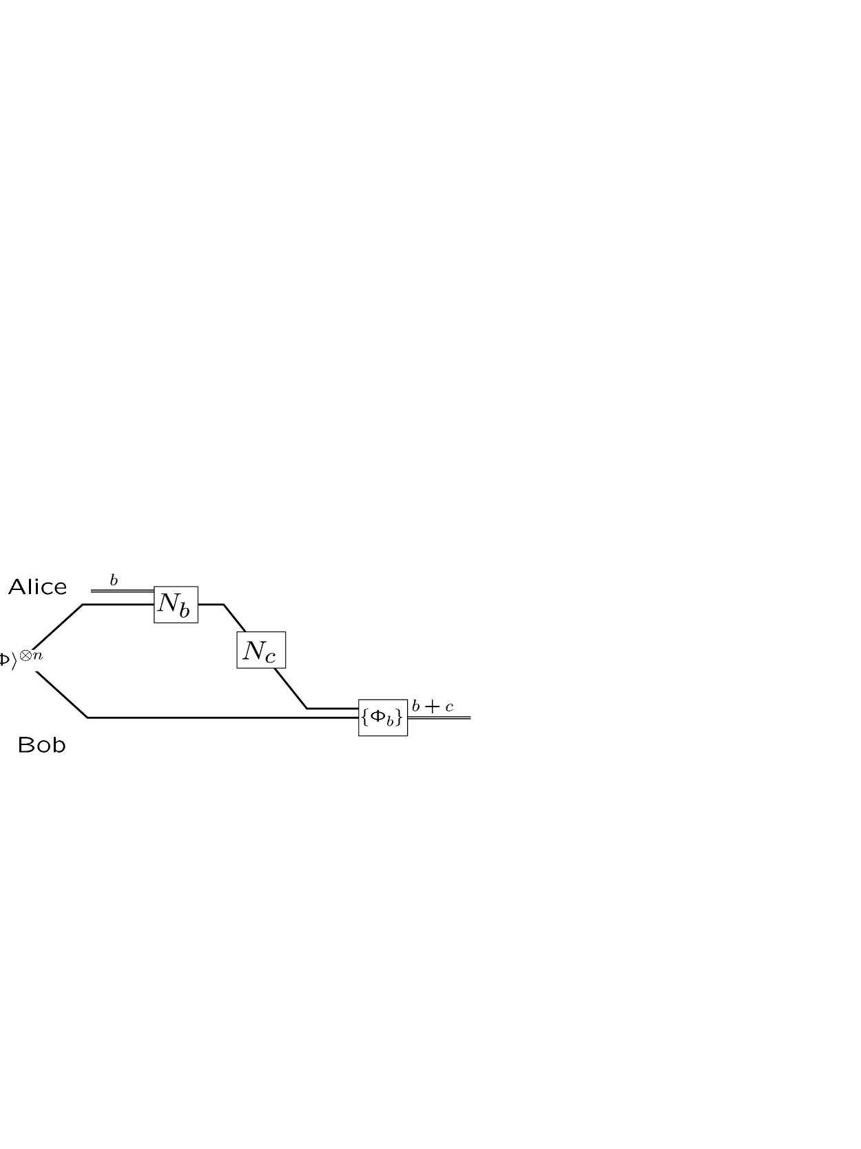
Figure 8: Reduction from an EACEC code to a classical code over $\mathbb{F}_{4}$.

Proof  We will show that superdense coding establishes an equivalence between a quantum Pauli error $N_{{\mathbf{c}}}$ and a classical error ${\mathbf{c}}$.

Assume ${\mathbf{c}}=0$, corresponding to no error. Alice superdense encodes ${\mathbf{b}}$ by performing $N_{{\mathbf{b}}}$ on her half of $|\Phi\rangle^{\otimes n}$. Bob performs a measurement in the $\{{|\Phi_{\mathbf{b}}\rangle\!\langle\Phi_{\mathbf{b}}|}:{\mathbf{b}}\in(\mathbb{F}_{4})^{n}\}$ basis, where $|\Phi_{\mathbf{b}}\rangle=(N_{\mathbf{b}}\otimes I)|\Phi\rangle$, thus decoding ${\mathbf{b}}$.

If the channel is $\hat{N}_{\mathbf{c}}$ for some ${\mathbf{c}}\in S$, then Alice’s effective encoding becomes $N_{\mathbf{c}}N_{\mathbf{b}}$ which is a representative of $[N_{{\mathbf{b}}+{\mathbf{c}}}]$. Bob’s measurement will reveal ${\mathbf{b}}+{\mathbf{c}}$ instead of ${\mathbf{b}}$. This is the message with a classical error ${\mathbf{c}}\in S$. The encoding preparation, followed by quantum error $\hat{N}_{\mathbf{c}}$ and decoding measurement, simulates the noisy classical channel ${\mathbf{b}}\mapsto{\mathbf{b}}+{\mathbf{c}}$. The theorem now follows, since the classical code can correct any error $c\in S$ . $\Box$

Thus there is a direct correspondence between $[n,k,d]_{4}$ classical codes and $[n,k,d;n]$ EACEC codes. On the other hand, in Section 3 we saw that an $[n,k,d]_{4}$ classical code defines an $[[n,2k-n+c,d;c]]$ EAQEC code. In the next subsection we show how to construct a variation on an $[[n,2k-n+c,d;c]]$ EAQEC code from an $[n,k,d;n]_{4}$ EACEC code via “coherification.”

5.2 Coherent EACEC codes

At this point we need to introduce one more resource, coherent communication [19]. Let $\{|0\rangle,|1\rangle\}$ denote a preferred basis for a qubit system. The isometric channel which implements the change of basis

$$\Delta_{2}:|i\rangle^{A}\mapsto|i\rangle^{A}|i\rangle^{B},\,\,i=0,1$$

is called the coherent bit (or cobit) channel. The superscript $A$ denotes a system held by Alice and $B$ denotes a system held by Bob. It is regarded as a coherent version of a classical bit channel. Viewing it as a resource, we use the symbol $[q\rightarrow q\,q]$. Coherifying a protocol is a broad notion marked by replacing classical communication by coherent communication [13, 19]. It was shown in [19] that superdense coding can be made coherent, i.e. that the following resource inequality holds:

$$[q\rightarrow q]+[q\,q]\geq 2[q\rightarrow q\,q].$$ (45)

Consider an $[n,k,d;n]$ EACEC code, given by (44). It can also be made coherent thanks to its connection to superdense coding. In other words, (44) can be upgraded to

$$\langle{\cal N}\rangle+n\,[q\,q]\geq 2k\,[q\rightarrow q\,q].$$ (46)

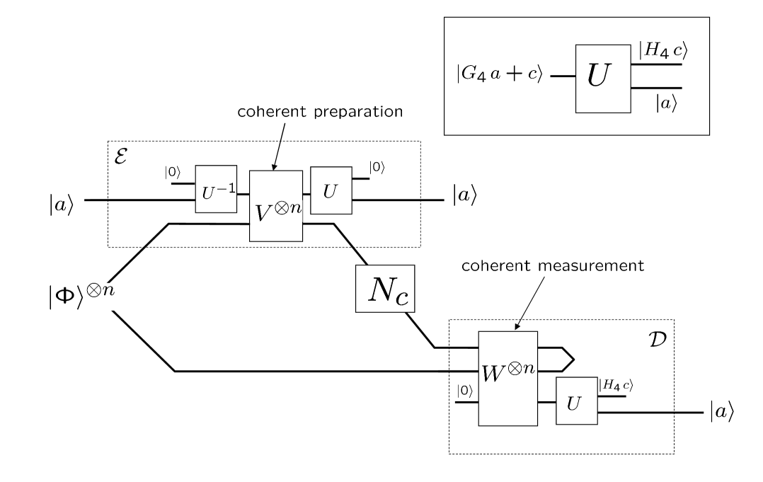
Figure 9: The circuit implementing a coherent EACEC code. The upper right hand corner defines $U$ in terms of the quaternary code with parity check matrix $H_{4}$ and generating matrix $G_{4}$.

An explicit circuit implementing this resource inequality is given in Figure 9. The states $\{|{\mathbf{a}}\rangle:{\mathbf{a}}\in(\mathbb{F}_{4})^{k}\}$ form a basis for a $2k$ qubit space. $\{N_{\mathbf{c}}\}$ is a Pauli matrix whose index ${\mathbf{c}}\in(\mathbb{F}_{4})^{n}$ is in the support of ${\cal N}$. $H_{4}$ is the $(n-k)\times n$ quaternary parity check matrix for the classical $[n,k,d]_{4}$ code which corrects all such ${\mathbf{c}}$. $G_{4}$ is the corresponding $n\times k$ generator matrix such that $H_{4}G_{4}={\bf 0}_{(n-k)\times k}$. The box in the upper right hand corner defines the $4^{n}\times 4^{n}$ unitary matrix $U$. There $G_{4}{\mathbf{a}}\in(\mathbb{F}_{4})^{n}$ is an encoded element ${\mathbf{a}}$ of $(\mathbb{F}_{4})^{k}$. The unitaries $V$ and $W$ are given by $V=\sum_{j\in\mathbb{F}_{4}}|j\rangle\langle j|\otimes N_{j}$ and

$$W(|\varphi\rangle|0\rangle)=\sum_{j\in\mathbb{F}_{4}}\langle\Phi_{+}|(N_{j}^{\dagger}\otimes I)|\varphi\rangle\,(|\Phi_{+}\rangle|j\rangle).$$

Harrow [19] also exhibited a coherent version of quantum teleportation [1], written as

$$2k\,[q\rightarrow q\,q]+k\,[q\,q]\geq k\,[q\rightarrow q]+2k\,[q\,q].$$ (47)

Figure 10 depicts a circuit implementing this resource inequality.

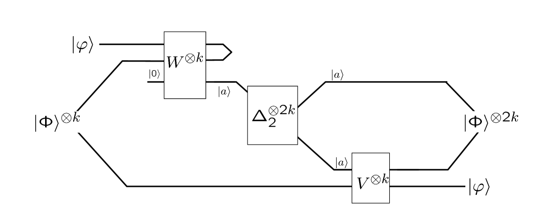
Figure 10: The circuit implementing coherent teleportation.

Combining (46) with (47) gives

$$\langle{\cal N}\rangle+(n+k)\,[q\,q]\geq k\,[q\rightarrow q]+2k\,[q\,q].$$ (48)

This differs from a hypothetical $[[n,k;n-k]]$ EAQEC code given by

$$\langle{\cal N}\rangle+(n-k)\,[q\,q]\geq k\,[q\rightarrow q]$$

in that an extra $2k\,[q\,q]$ is needed as a catalyst. We call this a type II $[[n,k;n-k;2k]]$ EAQEC code, and will refer to the EAQEC codes from Section 2 as type I EAQEC codes. A EAQEC code is not as versatile as regular EAQEC codes. The catalyst does not allow it to be converted into a catalytic QEC code, for example. Also, type II EAQEC codes appear to be limited to $\mathbb{F}_{4}$ construction.

As in the original Shannon theoretical result [13] (Figure 1), type II EAQEC codes (48) can be combined with superdense coding (18) to give a catalytic version of an EACEC code (44):

$$\langle{\cal N}\rangle+n\,[q\,q]+k\,[q\,q]\geq 2k\,[c\rightarrow c]+k\,[q\,q].$$

This does not hold for type I EAQEC codes of Section 2, unless $c$ equals its maximal value of $n-k$.

6 Bounds on performance

In this section we shall see that the performance of EAQEC codes is comparable to the performance of QEC codes (which are a special case of EAQEC codes).

The two most important outer bounds for QEC codes are the quantum Singleton bound [21, 29] and the quantum Hamming bound [16]. Given an $[[n,k,d]]$ QEC code (which is an $[[n,k,d;0]]$ EAQEC code), the quantum Singleton bound reads

$$n-k\geq 2(d-1).$$

The quantum Hamming bound holds only for non-degenerate codes and reads

$$\sum_{j=0}^{\lfloor\frac{d-1}{2}\rfloor}3^{j}{n\choose j}\leq 2^{n-k}.$$

The proofs of these bounds [29, 16] are easily adapted to EAQEC codes with $k-c$ playing the role of $k$. This was first noted by Bowen [5] in the case of the quantum Hamming bound, which now reads

$$\sum_{j=0}^{\lfloor\frac{d-1}{2}\rfloor}3^{j}{n\choose j}\leq 2^{n-k+c}.$$

The new quantum Singleton bound is

$$n-k+c\geq 2(d-1).$$

Note that the $\mathbb{F}_{4}$ construction connects the quantum Singleton bound to the classical Singleton bound $n-k\geq d-1$. An $[n,k,d]_{4}$ code saturating the classical Singleton bound implies an $[[n,2k-n+c,d;c]]$ EAQEC code saturating the quantum Singleton bound.

It is instructive to examine the asymptotic performance of quantum codes on a particular channel. A popular choice is the tensor power channel ${\cal N}^{\otimes n}$, where ${\cal N}$ is the depolarizing channel with Kraus operators $\{\sqrt{p_{0}}I,\sqrt{p_{1}}X,\sqrt{p_{2}}Y,\sqrt{p_{3}}Z\}$, for some probability vector ${\bf p}=(p_{0},p_{1},p_{2},p_{3})$.

It is well known that the maximal transmission rate $R=k/n$ achievable by a non-degenerate QEC code (in the sense of vanishing error for large $n$ on the channel ${\cal N}^{\otimes n}$) is equal to the hashing bound $R=1-H({\bf p})$. Here $H({\bf p})$ is the Shannon entropy of the probability distribution ${\bf p}$. This bound is attained by picking a random dual-containing code. However no explicit constructions are known which achieve this bound.

Interestingly, the $\mathbb{F}_{4}$ construction also connects the hashing bound to the Shannon bound for quaternary channels. Consider the quaternary channel $a\mapsto a+c$, where $c$ takes on values $0,\omega,1,\overline{\omega}$, with respective probabilities $p_{0},p_{1},p_{2},p_{3}$. The maximal achievable rate $R=k/n$ for this channel was proved by Shannon to equal $R=2-H({\bf p})$. An $[n,k]_{4}$ code saturating the Shannon bound implies an $[[n,2k-n+c;c]]$ CQEC code achieving the hashing bound! (Recall that the net rate of an $[[n,k;c]]$ CQEC code is defined as $R=(k-c)/n$.) Efficiently decodable modern classical codes, such as low-density parity check (LDPC) codes and turbo codes, are known to come very close to the Shannon bound. These codes are not at all guaranteed to be dual-containing [26], which means that no hashing bound attaining QEC code can be constructed from them. However, a catalytic QEC code can. Directly investigating the symplectic structure of such modern codes will reveal the size of the catalyst. We expect that bootstrapping the method from Figure 7 will enable us to construct a QEC code with similar properties.

7 The [[3,1,3;2]] EAQEC code

In this section, we will construct a $[[3,1,3;2]]$ EAQEC code and relate this code to Bowen’s earlier result [5]. Consider the classical $[3,1,3]$ quaternary code with parity check matrix

$$H_{4}=\left(\begin{array}[]{ccc}1&1&0\\ 1&0&1\end{array}\right).$$ (49)

Then

$$H=\gamma(\widetilde{H}_{4})=\left(\begin{array}[]{ccc|ccc}1&1&0&0&0&0\\ 1&0&1&0&0&0\\ 0&0&0&1&1&0\\ 0&0&0&1&0&1\end{array}\right).$$ (50)

Following the proof of Theorem 1.1, we have

$$\begin{array}[]{ccccccc}{\mathbf{u}}_{1}=&(1&1&0&0&0&0)\\ {\mathbf{u}}_{2}=&(0&0&0&1&1&0)\\ {\mathbf{u}}_{3}=&(1&1&1&0&0&0)\\ {\mathbf{v}}_{1}=&(0&0&0&1&0&1)\\ {\mathbf{v}}_{2}=&(1&0&1&0&0&0)\\ {\mathbf{v}}_{3}=&(0&0&0&1&1&1),\end{array}$$ (51)

and the hyperbolic pairs $({\mathbf{u}}_{1},{\mathbf{v}}_{1})$ and $({\mathbf{u}}_{2},{\mathbf{v}}_{2})$ span the rowspace of $H$. The simultaneous $+1$ eigenstate of the commuting operators $N_{{\mathbf{u}}_{i}}$, $i=1,2,3$, is

$$|\widetilde{000}\rangle=\frac{1}{\sqrt{2}}(|000\rangle+|110\rangle).$$

Then

$$\begin{split}|\widetilde{000}\rangle&=\frac{1}{\sqrt{2}}(|000\rangle+|110\rangle)\\ |\widetilde{001}\rangle&=N_{{\mathbf{v}}_{1}}|\widetilde{000}\rangle=(X\otimes I\otimes X)|\widetilde{000}\rangle=\frac{1}{\sqrt{2}}(|101\rangle+|011\rangle)\\ |\widetilde{010}\rangle&=N_{{\mathbf{v}}_{2}}|\widetilde{000}\rangle=(Z\otimes I\otimes Z)|\widetilde{000}\rangle=\frac{1}{\sqrt{2}}(|101\rangle-|011\rangle)\\ |\widetilde{011}\rangle&=N_{{\mathbf{v}}_{1}+{\mathbf{v}}_{2}}|\widetilde{000}\rangle=(Y\otimes I\otimes Y)|\widetilde{000}\rangle=\frac{1}{\sqrt{2}}(-|101\rangle+|011\rangle)\\ |\widetilde{100}\rangle&=N_{{\mathbf{v}}_{3}}|\widetilde{000}\rangle=(X\otimes X\otimes X)|\widetilde{000}\rangle=\frac{1}{\sqrt{2}}(|111\rangle+|001\rangle)\\ |\widetilde{101}\rangle&=N_{{\mathbf{v}}_{1}+{\mathbf{v}}_{3}}|\widetilde{000}\rangle=(I\otimes X\otimes I)|\widetilde{000}\rangle=\frac{1}{\sqrt{2}}(|010\rangle+|100\rangle)\\ |\widetilde{110}\rangle&=N_{{\mathbf{v}}_{2}+{\mathbf{v}}_{3}}|\widetilde{000}\rangle=(Y\otimes X\otimes Y)|\widetilde{000}\rangle=\frac{1}{\sqrt{2}}(-|111\rangle+|001\rangle)\\ |\widetilde{111}\rangle&=N_{{\mathbf{v}}_{1}+{\mathbf{v}}_{2}+{\mathbf{v}}_{3}}|\widetilde{000}\rangle=(Z\otimes X\otimes Z)|\widetilde{000}\rangle=\frac{1}{\sqrt{2}}(|010\rangle-|100\rangle)\end{split}$$ (52)

The encoding unitary $U_{\Upsilon}$ is therefore

$$U_{\Upsilon}=\frac{1}{\sqrt{2}}\left(\begin{array}[]{cccccccc}1&0&1&0&0&0&0&0\\ 0&0&0&0&1&0&1&0\\ 0&0&0&0&0&1&0&1\\ 0&1&0&1&0&0&0&0\\ 0&0&0&0&0&1&0&-1\\ 0&1&0&-1&0&0&0&0\\ 1&0&-1&0&0&0&0&0\\ 0&0&0&0&1&0&-1&0\end{array}\right).$$ (53)

The logical $0$ and $1$ codewords are

$$\begin{split}|0_{L}\rangle&=U_{\Upsilon}|0\rangle|\Phi_{+}\rangle^{\otimes 2}=\frac{1}{2}\left(|\widetilde{000}\rangle|00\rangle+|\widetilde{001}\rangle|01\rangle+|\widetilde{010}\rangle|10\rangle+|\widetilde{011}\rangle|11\rangle\right)\\ |1_{L}\rangle&=U_{\Upsilon}|1\rangle|\Phi_{+}\rangle^{\otimes 2}=\frac{1}{2}\left(|\widetilde{100}\rangle|00\rangle+|\widetilde{101}\rangle|01\rangle+|\widetilde{110}\rangle|10\rangle+|\widetilde{111}\rangle|11\rangle\right)\end{split}$$ (54)

Bowen’s code [5] can be obtained by applying the following unitary to the codewords given above

$$U_{B}=\frac{1}{2\sqrt{2}}\left(\begin{array}[]{cccccccc}1&-1&-1&-1&-1&1&1&1\\ -1&-1&-1&1&1&1&1&-1\\ 1&-1&1&1&-1&1&-1&-1\\ -1&-1&1&-1&1&1&-1&1\\ 1&-1&-1&-1&1&-1&-1&-1\\ 1&1&1&-1&1&1&1&-1\\ -1&1&-1&-1&-1&1&-1&-1\\ -1&-1&1&-1&-1&-1&1&-1\end{array}\right).$$ (55)

8 Table of codes

In [8] a table of best known QEC codes was given. Below we show an updated table which includes EAQEC codes.

$n\backslash{k-c}$	0	1	2	3	4	5	6	7	8	9	10
3	$2$	$\,\,\,2^{*}$	$1$	$1$
4	$\,\,\,3^{*}$	$2$	$2$	$1$	$1$
5	$3$	$3$	$2$	$\,\,\,2^{*}$	$1$	$1$
6	$4$	$3$	$2$	$2$	$2$	$1$	$1$
7	$3$	$3$	$2$	$2$	$2$	$\,\,\,2^{*}$	$1$	$1$
8	$4$	$3$	$3$	$3$	$2$	$2$	$2$	$1$	$1$
9	$4$	$\,\,\,4^{*}$	$3$	$3$	$2$	$2$	$2$	$\,\,\,2^{*}$	$1$	$1$
10	$\,\,\,5^{*}$	$4$	$4$	$3$	$3$	$2$	$2$	$2$	$2$	$1$	$1$

The entries with an asterisk mark the improvements over the table from [8]. All these are obtained from Proposition 3.1. The corresponding classical quaternary code is available online at http://www.win.tue.nl/$\sim$aeb/voorlincod.html.

The general methods from [8] for constructing new codes from old also apply here. Moreover, new constructions are possible since the dual-containing condition is lifted. An example is given by the following Theorem.

Theorem 8.1

a) Suppose an $[[n,{k},d;c]]$ code exists, then an $[[n+1,{k}-c+c^{\prime}-1,d^{\prime};c^{\prime}]]$ code exists for some $c^{\prime}$ and $d^{\prime}\geq d$; b) Suppose a non-degenerate $[[n,{k},d;c]]$ code exists, then an $[[n-1,{k}-c+c^{\prime}+1,d-1;c^{\prime}]]$ code exists for some $c^{\prime}$.

Proof  a) Let $H$ be the $(n-{k}+c\times 2n)$ parity check matrix of the $[[n,{k},d;c]]$ code. The parity check matrix of the new $[[n+1,{k}-c+c^{\prime}-1,d^{\prime};c^{\prime}]]$ is then

$$H^{\prime}=\left(\begin{tabular}[]{cc|cc}0 $\cdots$ 0&0&1 $\cdots$ 1&1\\ 1 $\cdots$ 1&1&0 $\cdots$ 0&0\\ &0&&0\\ \raisebox{2.15277pt}[0.0pt][0.0pt]{$H_{Z}$}&\vdots&\raisebox{2.15277pt}[0.0pt][0.0pt]{$H_{X}$}&\vdots\\ &0&&0\end{tabular}\right).$$ (56)

This corresponds to the classical construction of adding a parity check at the end of the codeword [27]. The additional rows ensure that errors involving the last qubit are detected. Sometimes the distance actually increases: for instance, the $[[8,0,4;0]]$ code is obtained from the $[[7,1,3;0]]$ code in this way.

b) We mimic the classical “puncturing” method [27]. Let $C$ be the $(n+{k}-c)$-dimensional subspace of $(\mathbb{Z}_{2})^{2n}$ corresponding to the $[[n,{k},d;c]]$ EAQEC code. Puncturing $C$ by deleting the first $Z$ and $X$ coordinate, we obtain a new “code” $C^{\prime}$ which is an $(n+{k}-c)$-dimensional subspace of $(\mathbb{Z}_{2})^{2(n-1)}$. This corresponds to an $[[n-1,{k}-c+c^{\prime}+1,d-1;c^{\prime}]]$ EAQEC code, as the minimum distance between the “codewords” of $C$ decreases by at most $1$. $\Box$

9 Discussion

Motivated by recent developments in quantum Shannon theory, we have introduced a generalization of the stabilizer formalism to the setting in which the encoder Alice and decoder Bob pre-share entanglement (EAQEC codes). We have traced the male side of family tree of quantum Shannon theory, from EAQEC codes (corresponding to the father protocol) to catalytic quantum codes (corresponding to the quantum capacity) and EACEC codes (corresponding to the classical EA-capacity). Moreover, EACEC codes can be made coherent, providing an alternative to the EAQEC construction from Section 2. The most obvious question is whether we can do the same for the female side of the family tree [13]. Preliminary results [24] give a positive answer to this question: entanglement distillation protocols assisted by quantum and classical communication can be constructed based on non-orthogonal symplectic codes.

There are two practical advantages of EAQEC codes over standard QEC codes:

1. They are much easier to construct from classical codes because they are not required to be dual-containing. This allows us to import the classical theory of error correction wholesale, including capacity-achieving modern codes. We plan to examine the performance of classical LDPC codes and turbo codes in the context of the catalyst size for EAQEC codes.

2. The entanglement used in the protocol is a strictly weaker resource than quantum communication. Thus comparing $[[n,k,d;c]]$ EAQEC codes to $[[n,k-c,d;0]]$ QEC codes is not being entirely fair to former. The pre-shared entanglement could have been obtained from a two way entanglement distillation protocol which achieve higher rates compared than one-way schemes. In this sense, a large value of the catalyst $c$ is viewed as advantageous, as it implies a higher qubit channel yield.

If one is interested in applications to fault tolerant quantum computation, where the resource of entanglement is meaningless, high values of $c$ are unwelcome because they require a long seed QEC code. We expect this obstacle to be overcome by bootstrapping.

Another fruitful line of investigation connects to quantum cryptography. Quantum cryptographic protocols, such as BB84, are intimately related to CSS QEC codes. In [25] it is shown that EAQEC analogues of CSS codes give rise to key expansion protocols which do not rely on the existence of long dual-containing codes.

We thank Graeme Smith for pointing us to references [6] and [15]. TAB acknowledges financial support from NSF Grant No. CCF-0448658, and TAB and MHH both received support from NSF Grant No. ECS-0507270. ID and MHH acknowledge financial support from NSF Grant No. CCF-0524811 and NSF Grant No. CCF-0545845.

References

- [1] C. H. Bennett, G. Brassard, C. Crépeau, R. Jozsa, A. Peres, and W. K. Wootters. Teleporting an unknown quantum state via dual classical and Einstein-Podolsky-Rosen channels. Phys. Rev. Lett., 70, 1993.
- [2] C. H. Bennett, D. P. DiVincenzo, J. A. Smolin, and W. K. Wooters. Mixed state entanglement and quantum error correction. Phys. Rev. A, 52:3824–3851, 1996. quant-ph/9604024.
- [3] C. H. Bennett, P. W. Shor, J. A. Smolin, and A. Thapliyal. Entanglement-assisted capacity of a quantum channel and the reverse Shannon theorem. IEEE Trans. Inf. Theory, 48, 2002. quant-ph/0106052.
- [4] C. H. Bennett and S. J. Wiesner. Communication via one- and two-particle operators on Einstein-Podolsky-Rosen states. Phys. Rev. Lett., 69:2881–2884, 1992.
- [5] G. Bowen. Entanglement required in achieving entanglement-assisted channel capacities. Phys. Rev. A, 66:052313, 2002. quant-ph/0205117.
- [6] S. Bravyi, D. Fattal, and D. Gottesman. GHZ extraction yield for multipartite stabilizer states. J. Math. Phys., 47:062106, 2006. quant-ph/0504208.
- [7] A. R. Calderbank, E. M. Rains, P. W. Shor, and N. J. A. Sloane. Quantum error correction and orthogonal geometry. Phys. Rev. Lett., 78:405–408, 1997. quant-ph/9605005.
- [8] A. R. Calderbank, E. M. Rains, P. W. Shor, and N. J. A. Sloane. Quantum error correction via codes over GF(4). IEEE Trans. Inf. Theory, 44:1369–1387, 1998. quant-ph/9608006.
- [9] A. R. Calderbank and P. W. Shor. Good quantum error-correcting codes exist. Phys. Rev. A, 54:1098–1105, 1996. quant-ph/9512032.
- [10] A. C. da Silva. Lectures on symplectic geometry. Springer-Verlag, Berlin, 2001.
- [11] I. Devetak. The private classical capacity and quantum capacity of a quantum channel. IEEE Trans. Inf. Theory, 51(1):44–55, 2005. quant-ph/0304127.
- [12] I. Devetak, A. W. Harrow, and A. Winter. A resource framework for quantum Shannon theory, 2005. quant-ph/0512015.
- [13] I. Devetak, A. W. Harrow, and A. J. Winter. A family of quantum protocols. Phys. Rev. Lett., 93, 2004. quant-ph/0308044.
- [14] I. Devetak and A. Winter. Distilling common randomness from bipartite quantum states. IEEE Trans. Inf. Theory, 50:3138–3151, 2003. quant-ph/0304196.
- [15] D. Fattal, T. S. Cubitt, Y. Yamamoto, S. Bravyi, and I. L. Chuang. Entanglement in the stablizer formalism, 2004. quant-ph/0406168.
- [16] D. Gottesman. A class of quantum error correcting codes saturating the quantum Hamming bound. Phys. Rev. A, 54:1862, 1996.
- [17] D. Gottesman. A theory of fault-tolerant quantum computation. Phys. Rev. A, 57:127–137, 1998. quant-ph/9702029.
- [18] M. Hamada. Information rates achievable with algebraic codes on quantum discrete memoryless channels, 2002. quant-ph/0207113.
- [19] A. W. Harrow. Coherent communication of classical messages. Phys. Rev. Lett., 92, 2004. quant-ph/0307091.
- [20] G. D. Forney Jr., M. Grassl, and S. Guha. Convolutional and tail-biting quantum error-correcting codes, 2005. quant-ph/0511016.
- [21] E. Knill and R. Laflamme. A theory of quantum error correcting codes. Phys. Rev. A, 55:900, 1997. quant-ph/9604034.
- [22] R. Laflamme, C. Miquel, J.-P. Paz, and W. H. Zurek. Perfect quantum error-correction code. Phys. Rev. Lett., 77:198–201, 1996. quant-ph/9602019.
- [23] S. Lloyd. Capacity of the noisy quantum channel. Phys. Rev. A, 55, 1996. quant-ph/9604015.
- [24] Z. Luo and I. Devetak. Catalytic entanglement distillation, 2006. In preparation.
- [25] Z. Luo and I. Devetak. Quantum key expansion from non-orthogonal codes, 2006. quant-ph/0608029.
- [26] D. J. C. MacKay, G. Mitchison, and P. L. McFadden. Sparse-graph codes for quantum error correction. IEEE Trans. Inf. Theory, 50:2315–2330, 2004.
- [27] F.J. MacWilliams and N.J.A. Sloane. The Theory of Error-Correcting Codes. Elsevier, Amsterdam, 1977.
- [28] M. A. Nielsen and I. L. Chuang. Quantum Computation and Quantum Information. Cambridge University Press, New York, 2000.
- [29] J. Preskill. Lecture notes for physics 229: Quantum information and computation, 1998. http://www.theory.caltech.edu/people/preskill/ph229.
- [30] C. E. Shannon. A mathematical theory of communication. Bell System Tech. Jnl., 27:379–423, 623–656, 1948.
- [31] P. W. Shor. Scheme for reducing decoherence in quantum computer memory. Phys. Rev. A, 52:2493–2496, 1995.
- [32] P. W. Shor. The quantum channel capacity and coherent information. MSRI workshop on quantum computation, 2002.
- [33] A. M. Steane. Error-correcting codes in quantum theory. Phys. Rev. Lett., 77:793–797, 1996.