Classical search algorithm with resonances in $\sqrt{N}$ cycles

Abstract

In this work we use the wave equation to obtain a classical analog of the quantum search algorithm and we verify that the essence of search algorithms resides in the establishment of resonances between the initial and the serched states. In particular we show that, within a set of $N$ vibration modes, it is possible to excite the searched mode in a number of steps proportional to $\sqrt{N}$.
Keywords: search algorithm; quantum optics; quantum information

I Introduction

It has been shown that a quantum search algorithm is able to locate a marked item from an unsorted list of $N$ elements in a number of steps proportional to $\sqrt{N}$, instead of proportional to $N$ as is the case for the usual algorithms employed in classical computation. The most well studied quantum search algorithm is the one due to Grover Chuang , where the search is performed by alternatively shifting the phase of the searched for state, and amplifying its modulus. A continuous time version of the original Grover algorithm has been described by Farhi and Gutmann Farhi . In a recent work alejo1 , we have presented an alternative continuous time quantum search algorithm, in which the search set is taken from the set of eigenvectors of a particular hamiltonian. The search is performed through the application of a perturbation which leads to the appearance of a resonance between the initial and the searched state. That study also provided a new insight on the connections between discrete and continuous time search algorithms. Our search algorithm can be implemented using any Hamiltonian with a discrete energy spectrum. However, we would like to emphasize that the possibility of establishing a resonance between two states is an intrinsic property of oscillatory motions in general and not an exclusive property of quantum mechanics as described through the Schrödinger equation, as in our algorithm.

A link between quantum computation and classical optical waves has been well established by several authorsCerf ; Roldan ; Puentes ; Pittman ; Bhatta ; Jennifer . It is possible to simulate the behavior of some simple quantum computers using classical optical waves. Although the necessary hardware grows exponentially with the number of qubits that are simulated, and thus these simulations are not efficient, optical simulations could still be very useful. In fact, as some simulations of quantum algorithms employ optical simulations, a classical analogue of such a quantum search algorithm might be a valuable tool to test the functioning of the optical system as a computer.

In this work we present a continuous time search algorithm, which is controlled by a classical wave equation, showing explicitly, once again, that the search algorithm is essentially a resonance phenomenon between the initial and the searched states alejo1 ; Grover2 . The paper is organized as follows: in the next section we briefly describe our quantum search algorithm. Then, in section 3, we develop the search model using the ordinary wave equation. In section 4 we present results obtained with this model. We end by discussing these results and extracting conclusions, in the last section of this work.

II Quantum search algorithm

We consider a continuous time quantum search algorithm which is controlled by a time dependent Hamiltonian $H$. The wavefunction $|\Psi(t)\rangle$ satisfies the Schrödinger equation

$$i\frac{\partial|\Psi(t)\rangle}{\partial t}=H\text{ }|\Psi(t)\rangle,$$ (1)

where $H=H_{0}+V(t)$ and we have taken the Planck constant $\hbar=1$. Here $H_{0}$ is a known nondegenerate time-independent Hamiltonian with a discrete energy spectrum $\left\{\varepsilon_{n}\right\}$ and eigenstates $\left\{|n\rangle\right\}$. $V(t)$ is a time-dependent potential that shall be defined below. We then consider a subset N of $\left\{|n\rangle\right\},$ formed by $N$ states, which will be our search set. Let us call $|s\rangle$ the unknown searched state in N whose energy $\varepsilon_{s}$ is given. We assume that it is the only state in N with that value of the energy. Therefore, knowing $\varepsilon_{s}$ is, in our algorithm, equivalent to the action of “marking” the searched state, in Grover’s algorithm. The potential $V$ that produces the coupling between the initial and the searched states, is defined as alejo1

$$V(t)=\left|p\right\rangle\left\langle j\right|\exp\left(i\omega_{sj}t\right)+\left|j\right\rangle\left\langle p\right|\exp\left(-i\omega_{sj}t\right)$$ (2)

where the eigenstate $|j\rangle$, with eigenvalue $\varepsilon_{j}$, is the initial state of the system and it is chosen so that it does not belong to the subset N. Above, $\left|p\right\rangle\equiv\frac{1}{\sqrt{N}}{\displaystyle\sum\limits_{n\in{\mathbf{N}}}}|n\rangle$ is an unitary vector which can be interpreted as the average of the set of vectors in N, and $\omega_{sj}\equiv\varepsilon_{j}-\varepsilon_{s}$. This definition ensures that the interaction potential is hermitian, that the transition probabilities $W_{nj}\equiv\left|\left\langle n|V(t)|j\right\rangle\right|^{2}=\frac{1}{N}$, from state $|j\rangle$ to any state of the set N are all equal, and finally, that the sum of the transition probabilities verifies ${\displaystyle\sum\limits_{n\in\mathbf{N}}}W_{nj}=1$.

Figure 1: (a) Initial configuration of the system: all $N$ pendulums at rest, except pendulum $j$. (b) Situation after $\sqrt{N}$ cycles: most of the energy was tranferred to the searched pendulum $s$.

The objective of the algorithm is to find the eigenvector $|s\rangle$ whose transition energy from the initial state $|j\rangle$ is the Bohr frequency $\omega_{sj}$. At this point we consider important to make a digression to visualize the way the perturbation potential $V(t)$ operates on the system. To better understand the process, let us consider a classical system composed of $N$ pendulums of different lengths, and, consequently, different oscillating frequencies. The search problem, illustrated in fig. 1, consists of identifying the pendulum $s$ with a given frequency of oscillation $\omega_{s}$. To perform the search, one suspends all the pendulums from the same beam, and puts to oscillate one of the pendulums, $j$. By applying a periodical force with frequency $\omega_{j}-\omega_{s}$, which may be derived from a potential $V(t)$, the sought after pendulum $s$ receives, after some time, most of the oscillation energy of the pendulum $j$, so it may be readily identified. This system, closely related to the one proposed by Grover Grover2 , also has the property that the identification is performed through the gradual exchange of energy between the oscillators, without a net external energy input.

Returning to the quantum search problem, the wavefunction $|\Psi(t)\rangle$ appearing in Schrödinger’s eq. (1) may be expressed as an expansion on the eigenstates $\{|n\rangle\}$ of $H_{0}$,

$$|\Psi(t)\rangle=\sum_{m}a_{m}(t)\exp\left(-i\varepsilon_{m}t\right)|m\rangle.$$ (3)

The time dependent coefficients $a_{m}(t)$ have initial conditions $a_{j}(0)=1$, $a_{m}(0)=0$ for all $m\neq j$. After solving the Schrödinger equation, the probability distribution results in,

$$P_{j} \simeq\cos^{2}(\Omega\ t)\ ,$$

$$P_{s} \simeq\sin^{2}(\Omega\ t)\ ,$$ (4)

$$P_{n} \simeq 0,\text{ }n\neq j\text{ and }n\neq s,$$

where $\Omega=1/\sqrt{N}$. From these equations it is clear that for $\tau=\pi/(2\Omega)$ a measurement yields the searched state with a probability very close to one. This approach is valid as long as all the Bohr frequencies satisfy $\omega_{nm}\gg\Omega$ and, in this case, our method behaves qualitatively like Grover’s.

III Search algorithm using classical waves

In this section we build a classical search algorithm which is controlled by a classical wave equation with an added perturbation. The task of this algorithm is, starting from an initial oscillation mode, to excite the searched mode, whose frequency is known, in $O(\sqrt{N})$ steps. The unperturbed wavefunction $\Psi(x,t)$ satisfies the ordinary wave equation in one spacial dimension,

$$\frac{\partial^{2}\Psi(x,t)}{\partial t^{2}}=c^{2}\frac{\partial^{2}\Psi(x,t)}{\partial x^{2}},$$ (5)

where $c$ is the constant wave velocity. This equation plays the same role as the Schrödinger equation in the algorithm shown in the previous section. From eq. (5) we define the basis on which the algorithm is built. Let us call $L$ the length of the region where the wave equation is solved. Then the canonical basis is given by the modes $\exp(-i\omega t)\sin(Kx)$ where $K$ is the wave number and $\omega$ is the circular frequency, connected through the dispersion relation $c=\omega/K$. In this case, the wave number and the frequency are of the form $K_{n}=K_{0}n$ and $\omega_{n}$ $=\omega_{0}n$ respectively, where $n$ is an integer, $K_{0}=2\pi/L$ and $\omega_{0}$ $=cK_{0}$.

As the analogue of the Schrödinger equation eq.(1) with the complete Hamiltonian $H=H_{0}+V(t)$ we consider the wave equation with a perturbative force term,

$$\frac{\partial^{2}\Psi(x,t)}{\partial t^{2}}=c^{2}\frac{\partial^{2}\Psi(x,t)}{\partial x^{2}}+c\omega_{0}\frac{\partial\left(V(t)T\Psi(x,t)\right)}{\partial x}$$ (6)

where $V(t)$ is a external time depend perturbative potential. The solution of eq. (6) can be expressed as a linear combination of the oscillation modes, of eq. (5)

$$\Psi(x,t)=\sum_{n}a_{n}(t)\exp(-i\omega_{n}t)\sin(K_{n}x),$$ (7)

where the coefficients are

$$a_{n}(t)=\exp(i\omega_{n}t)\frac{2}{L}\int\limits_{0}^{L}\Psi(x,t)\sin(K_{n}x)\text{ }dx.$$ (8)

In order for the algorithm to work, the operator $T$ in eq.(6) is defined as

$$T\Psi(x,t)=\sum_{n}a_{n}(t)\exp(-i\omega_{n})\cos(K_{n}x).$$ (9)

In order to obtain a greater connection with the previous section, we shall now adopt the Dirac notation for the coordinate space $|x\rangle$, and for momentum space $|n\rangle$. In this framework, the solution of the wave function can be expressed as

$$|\Psi\rangle=\sum_{n}a_{n}(t)\exp\left(-i\omega_{n}t\right)|n\rangle,$$ (10)

where we can write

$$a_{n}(t)=\frac{2\exp\left(i\omega_{n}t\right)}{L}\int\limits_{0}^{L}dx\left\langle n|x\right\rangle\left\langle x|\Psi\right\rangle,$$ (11)

with $\left\langle n|x\right\rangle=\sin(K_{n}x)$.

Once again, the task of the algorithm is to excite the oscillation mode $|s\rangle$ starting from the initial mode $|j\rangle$, with the transition frequency $\omega_{sj}\equiv\omega_{j}-\omega_{s}$. To perform this task, we choose as perturbation potential to excite the resonance between the initial and searched states the classical analogue of the one given by eq.(2). In our mixed notation, this time depended perturbation is

$$V(t)\Psi(x,t)\equiv\left\langle x|V(t)|\Psi\right\rangle=\sum_{n}\left\langle n|V(t)|\Psi\right\rangle\sin\left(K_{n}x\right),$$ (12)

where

$$\left\langle n|V(t)|\Psi\right\rangle =\frac{1}{\sqrt{N}}\{\left(1-\delta_{nj}\right)a_{j}(t)\exp\left(i\omega_{sj}t\right)$$ (13)

$$+\delta_{nj}\exp\left(-i\omega_{sj}t\right)\sum_{l\in\mathbf{N}}a_{l}(t)\exp\left(-i\omega_{l}t\right)\}.$$

The last equation has been obtained from eqs.(2,3). Using eqs.(7,12,13) in eq.(6) and projecting the result on the mode $n$ the following set of equations for the amplitudes $a_{n}(t)$ are obtained

$$\frac{d^{2}a_{n}(t)}{dt^{2}}-2i\omega_{n}\frac{da_{n}(t)}{dt} =-\frac{\omega_{0}}{\sqrt{N}}\{\omega_{n}\left(1-\delta_{nj}\right)a_{j}(t)\exp\left(i\omega_{sn}t\right)$$ (14)

$$+\omega_{j}\delta_{nj}\sum_{l\in\mathbf{N}}a_{l}(t)\exp\left(i\omega_{ls}t\right)\}.$$

These equations will be solved in the next section but meanwhile we address the question of their qualitative behavior. The eqs.(14) involve two time scales, a fast scale associated with the frequencies $\omega_{n}$, and a slow scale associated with the amplitudes $a_{n}(t)$. In a time interval larger than a characteristic time of the fast scale, the most important terms are those that have a very small phase, as the others average to zero. In this approximation the previous set of equations becomes

$$\frac{da_{j}(t)}{dt} \simeq-i\Omega a_{s}(t),$$

$$\frac{da_{s}(t)}{dt} \simeq-i\Omega a_{j}(t),$$ (15)

$$\frac{da_{n}(t)}{dt} \simeq 0\text{ for all }n\neq s,j;$$

where $\Omega=\omega_{0}/(2\sqrt{N})$. These equations represent two coupled oscillators where the coupling is established between the initial and the searched states. Solving them with initial conditions $a_{j}(0)=1$, $a_{s}(0)=0$ we obtain

$$a_{j}(t) \simeq\cos(\Omega t),$$

$$a_{s}(t) \simeq i\sin(\Omega t).$$ (16)

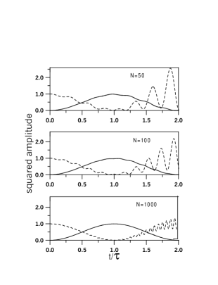
Figure 2: Time evolution of the squared amplitude of the initial state (dashed line) and the searched state (full line) for different number of modes $N$. The frequencies $\omega_{n}$ are taken with $n=1,2,3,...,N$.

It is important to note that the previous approach is valid only if all the frequencies verify $\omega_{n}\gg\Omega$. The amplitude of the searched state is maximum at the time $\tau\equiv\pi\sqrt{N}/\omega_{0}.$ This time is equivalent, in the Grover algorithm, to the optimal time to perform the measurement. Then, when the previous approximations are valid, our method behaves qualitatively like Grover’s. The time $\tau$ has a different prefactor than the searching time of the Grover algorithm,Chuang but this difference is not important because the resonance potential eq.(2) can be adjusted through multiplication by a constant factor.

IV Numerical results

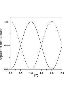
Figure 3: Squared amplitude of the initial state (dashed line) and the searched state (full line) as a function of time for $N=100$ modes. The frequencies $\omega_{n}$ are taken with $n=1,4,9,...,N^{2}$.

We have integrated numerically eqs.(14) with initial conditions $a_{j}(0)=1$, $a_{n}(0)=0$ for all $n\neq j$, and have verified that the solutions so obtained are independent of the remaining initial conditions for the derivatives $\frac{da_{j}(0)}{dt}$and $\frac{da_{s}(0)}{dt}$. The calculations were performed using a standard fourth order Runge-Kutta algorithm. Choosing an arbitrary frequency for the searched mode, we follow the dynamics of the set N. We have verified for several values of $N$ that the most important coupling is between the initial and the searched mode; other couplings being negligible as discussed in the previous section. We worked with two types of sets N, in the first set the mode frequencies $\omega_{n}=\omega_{0}n$ are taken with $n=1,2,3,...,N$ and in the second set with $n=1,4,9,...,N^{2}$. The square of the amplitude of the searched and the initially loaded modes are shown for the first set in Fig.2. The temporal evolution was normalized to the characteristic time $\tau$. Each panel shows the square of the amplitude for $N=50,100,1000$ modes respectively. From this figure, it is clear that the amplitudes of the initial mode and the searched mode alternate in time, as in the Grover algorithm.

The time at which the squared amplitude of the searched state is maximum and its value is very near one agrees with our theoretical prediction $\tau$. The agreement is much improved when $N$ increases because the condition $\Omega<<\omega_{nm}$ is better satisfied as $\Omega\sim 1/\sqrt{N}$. When $t\sim 2\tau$ the amplitude of the initial mode shows strong oscillations which decrease as the inverse of the search set size. We also observe that the frequency of these oscillations increases  with $N$.

Fig.3 shows the squared amplitude of the initial and the searched modes as a function of time for the second set. In this case the calculation agrees with the theoretical prediction for all $N>10$, and thus we have displayed only the calculation for $N=100$.

The search algorithm dynamics for the two sets, are rather similar. The differences observed are due to the properties of their frequency spectra. While the frequency spectrum of the first set increases linearly with the mode number, the frequency of the second set has a quadratic growth. Then in the first set, an additional interference effect must be expected because many more frequencies $\omega_{sn}$ have the same value for different values of $s$ and $n$ in the case of the first set than in the case of the second set. In this last case the frequencies $\omega_{sn}$ behave pseudorandomly and the additional interferences do not appear.

V Conclusions

We have developed a search algorithm using a classical wave equation with perturbation. This algorithm behaves like the Grover algorithm, in particular the optimal search time is proportional to the square root of the size of the search set and the probability to find the searched state oscillates periodically in time. The efficiency of this algorithm depends on the spectral density of frequencies of the set where the search is made. A larger separation between frequency levels maximizes the probability of the searched state and allows for a better precision. Nevertheless the classical implementation of this algorithm requires $N$ oscillation modes, whereas in a quantum system the implementation will only need $\log_{2}$ $N$ qubitsGrover2 .

Presently most of the attention is devoted to the development of quantum computational devices. In particular, there have been several recent attempts to employ optical simulations to run quantum algorithms (Cerf ; Bhatta ; Puentes ). These studies suggest that such optical implementations are possible for small systems with the presently available technology. Here, we have developed a general classical analogue of a quantum search algorithm which operates in the same way as the one implemented in the quantum case through optical devices. Thus, our work not only helps to understand the essence of the quantum algorithm, but also may serve as a testing ground for practical implementation of optical computational systems. Certainly much further experimental and theoretical work will be needed to develop the practical applications of this algorithm.

We acknowledge useful comments made by S. Barreiro, A. Lezama and V. Micenmacher, and financial support from PEDECIBA and PDT S/C/IF/54/5. R.D. acknowledges partial financial support from the Brazilian National Research Council (CNPq) and FAPERJ (Brazil). A.R and R.D. acknowledge financial support from the Brazilian Millennium Institute for Quantum Information.

References

- (1) M. Nielssen and I. Chuang, Quantum Computation and Quantum Information, Cambridge University Press, 2000.
- (2) E. Farhi and S. Gutmann Phys. Rev. A 57, 2403 (1998)
- (3) A. Romanelli, A. Auyuanet, R. Donangelo. Physica. A,(2005) (in press) also in quant-ph/0502161.
- (4) N. J. Cerf, C. Adami and P. G. Kwiat Phys. Rev. A 57, 3, R1477 (1998)
- (5) P.L.Knight, E. Roldán and J. E. Sipe, Phys. Rev. A 68, 020301(R) (2003); ibid. Optics Comm. 227, 147 (2003); E. Roldán and J. C. Soriano, quant-ph/0503069
- (6) G. Puentes, C. La Mela, S. Ledesma, C. Iemmi, J.P. Paz and M.Saraceno Phys. Rev. A 69, 042319 (2004)
- (7) T. B. Pittman, B. C. Jacobs and J. D. Franson Phys. Rev. A 71, 032307 (2005)
- (8) N. Bhattacharya, H.B. vanLindenvandenHeuvell, and R. J. C. Spreeuw, Phys. Rev. Lett. 88, 137901 (2002)
- (9) J.L. Dodd, T.C. Ralph and G. J. Milburn, Phys. Rev. A 68, 042328 (2003)
- (10) L. K. Grover, A.M. Sengupta, Phys. Rev. A 65, 032319 (2002), quant-ph/0109123.