Analysis of an experimental quantum logic gate
by complementary classical operations

Abstract

Quantum logic gates can perform calculations much more efficiently than their classical counterparts. However, the level of control needed to obtain a reliable quantum operation is correspondingly higher. In order to evaluate the performance of experimental quantum gates, it is therefore necessary to identify the essential features that indicate quantum coherent operation. In this paper, we show that an efficient characterization of an experimental device can be obtained by investigating the classical logic operations on a pair of complementary basis sets. It is then possible to obtain reliable predictions about the quantum coherent operations of the gate such as entanglement generation and Bell state discrimination even without performing these operations directly.

1 Introduction: Quantum Computation Processes

Within recent years, quantum computation has become a well established field of research in both experimental and theoretical physics. At the heart of this field is the notion that the highly entangled correlations of many-particle quantum systems could be used as a tool to efficiently solve problems of equally challenging complexity. In order to convert a quantum system from a mere object of observation into a problem solving tool, it is necessary to establish a nearly complete control over quantum processes at the microscopic level.

In close analogy to conventional computation, the method of establishing this high level of control over large quantum systems is to assemble the quantum systems from the smallest possible element offered by quantum theory, the two level system. For obvious reasons, this two level system is then referred to as a quantum bit or qubit. However, its physical properties are better visualized by the analogy with the three dimensional spin of a spin-1/2 system. In fact, one possible explanation for the efficiency of quantum computation is the fact that the possibilities of rotating a spin are infinite, while a classical bit can only be flipped. Intriguingly, quantum mechanics smoothly connects these seemingly contradictory aspects of reality in a single consistent theory.

In principle, it is possible to construct a universal quantum computer using only local spin rotations and a single well-defined interaction [1]. One such well-defined interaction between two qubits is the quantum controlled-NOT gate. When observed in the computational basis (usually associated with the $z$-component in the spin analogy), this gate performs a classical controlled-NOT logic operation. However, it is completely quantum coherent, so its actual performance is far more complex than that of its classical namesake.

Since the successful realization of a quantum controlled-NOT would enable universal quantum computation, a significant amount of experimental effort has been devoted to this goal. (see ref. [2] to [13] for examples.) However, experimental realizations are never identical to the ideal device described by theory. In order to demonstrate that an experimental device really performs the intended function, it needs to be tested. For classical logic gates, such a test is straightforward, since the number of possible operations is finite. But for operations on qubits, the possibility of arbitrarily small phase shifts implies that the number of possible quantum coherent operations is in principle infinite. Therefore, the experimental test of a quantum gate requires a somewhat deeper understanding of the essential features of general quantum operations. In particular, we need to go beyond the rather fuzzy image of quantum coherence and the associated “parallelism” of quantum superpositions, towards a more specific approach based on the observable features of quantum devices.

In this review, we briefly introduce the proper theoretical description of experimental quantum processes. We then show that the essential features of a quantum process can be defined in terms of only two complementary operations [14] and derive estimates for the quantum process fidelity and the entanglement capabilities based on the corresponding complementary classical fidelities. Finally, we present a recently realized optical controlled-NOT gate [13] and show how information about the actual device performance can be obtained from the experimental data.

2 Theoretical Description of Noisy Quantum Operations

Ideally, a quantum operation can be represented by a unitary operator $\hat{U}_{0}$ acting on the input state $\mid\psi_{\mbox{in}}\rangle$ in the $d$-dimensional Hilbert space of the quantum system. Since all quantum states can be expanded in terms of a complete orthogonal basis set $\{\mid n\rangle\}$, the effect of the unitary operation on an arbitrary input state is completely defined by its effects on such a set of $d$ basis states,

$$\hat{U}_{0}\mid n\rangle=\mid f_{n}\rangle.$$ (1)

Because the operation is unitary, the output states $\{\mid f_{n}\rangle\}$ also form an orthogonal basis set. The quantum operation is thus completely deterministic and leaves no room for unpredictable errors. In particular, it should be noted that the phases of the states $\mid f_{n}\rangle$ are also defined by eq. (1), so that the unitary transformation actually defines much more than the transformation of an eigenvalue $n$ to a corresponding eigenvalue $f_{n}$.

Obviously, it is very difficult to realize a nearly deterministic error free quantum operation experimentally. The idealized description given by a single unitary operation $\hat{U}_{0}$ is therefore not normally sufficient to describe noisy experimental processes. Instead, we have to assume that the actual process $\hat{A}_{m}$ acting on the input state $\mid\psi_{\mbox{in}}\rangle$ may fluctuate randomly and is not necessarily unitary. If the probability distribution over possible processes $\hat{A}_{m}$ is given by $p_{m}$, the output state is described by a mixed state density matrix [15],

$$\hat{\rho}_{\mbox{out}}=\sum_{m}p_{m}\hat{A}_{m}\mid\psi_{\mbox{in}}\rangle\langle\psi_{\mbox{in}}\mid\hat{A}_{m}^{\dagger}.$$ (2)

In general, any reproducible quantum process can be represented in such a form. However, if the precise source of errors is unknown, it is not possible to identify a unique set of operations $\hat{A}_{m}$. For the experimental evaluation of quantum processes, it is therefore more useful to find a representation that does not depend on the specific error syndromes $\hat{A}_{m}$.

It is in fact possible to express any noisy process in a $d$-dimensional Hilbert space in terms of an orthogonal set of $d^{2}$ operators ${\Lambda_{i}}$ by considering the $d\times d$ matrices representing the operators as vectors in a $d^{2}$-dimensional vector space [15, 16]. An ideal process can then be expressed as

$$\hat{A}_{m}=\sum_{i}c_{i}\hat{\Lambda}_{i},$$ (3)

and any noisy process $E$ can be described by a process matrix with elements $\chi_{ij}$, so that

$$\hat{\rho}_{\mbox{out}}=E(\hat{\rho}_{\mbox{in}})=\sum_{i,j}\chi_{ij}\hat{\Lambda}_{i}\hat{\rho}_{\mbox{in}}\hat{\Lambda}_{j}^{\dagger}.$$ (4)

Each process can thus be decomposed into a finite set of orthogonal processes $\{\hat{\Lambda}_{i}\}$, and the complete process is then defined by its process matrix elements $\chi_{ij}$.

In principle, the complete $d^{4}=16^{N}$ process matrix elements can always be evaluated by measuring the output statistics of a sufficient number of non-orthogonal input states [15]. This approach, called quantum process tomography, treats the quantum process as a black box, requiring no further assumptions about the intended process itself. In order to test a specific quantum operation however, it may be more useful to formulate the process matrix in terms of basis processes $\{\hat{\Lambda}_{i}\}$ that are close to experimentally observable error syndromes of the device. As we show in the following, it is then possible to obtain useful information about the device performance without an abstract analysis of the huge amount of data required for complete quantum process tomography.

3 Classification of Quantum Errors

For qubits, each error can be expanded in terms of products of errors acting on a single qubit, and the single qubit errors can be expressed in terms of the identity $I$ and the three Pauli matrices, $X$, $Y$, $Z$ [15, 16]. Using the spin analogy, these errors correspond to spin flips (rotations of 180 degrees) around the $x$-, $y$- and $z$-axis, respectively. An $N$-qubit system is thus characterized by the $N$-qubit identity $\hat{F}_{0}$ and $4^{N}-1$ spin flip errors, $\hat{F}_{i}$.

If the intended operation is $\hat{U}_{0}$, errors will be detected by comparing the output qubit statistics with the ideal operation. It is therefore useful to characterize the errors with reference to $\hat{U}_{0}$ as output errors $\hat{U}_{i}=\hat{F}_{i}\hat{U}_{0}$. The noisy process is then described by

$$E(\hat{\rho}_{\mbox{in}})=\sum_{i,j}\chi_{ij}\hat{U}_{i}\hat{\rho}_{\mbox{in}}\hat{U}_{j}^{\dagger},$$ (5)

where the diagonal elements $\chi_{ii}$ of the process matrix now correspond to the distribution of spin-flip errors in the output. It is thus possible to identify experimentally observed output errors directly with a group of theoretical error syndromes and their corresponding process matrix elements.

We now have a convenient mathematical form for the representation of errors in a quantum operation. However, we still need to determine the errors experimentally, so it is necessary to consider the observable effects of the errors for a given set of output states. Since most quantum information processes are formulated in the computational basis defined by the eigenvalues of $Z$, it is useful to start by considering an operation which produces the $Z$ basis states in the output, $\mid f_{n}\rangle=\mid Z_{1},Z_{2},\ldots\rangle$. In the $Z$ basis, the operators $X$ and $Y$ represents bit flips, and the operators $I$ and $Z$ preserve the qubit value. $Y$ and $Z$ also change the phase relation between the qubit states, but this phase change cannot be observed in the $Z$ basis. Therefore, it is not possible to distinguish $I$ from $Z$ or $Y$ from $X$ when the output is measured in the $Z$ basis.

Most importantly, a quantum device that always produces the correct $Z$ output may still have phase errors that destroy the quantum coherence between the outcomes. In fact, there are a total of $2^{N}$ mutually orthogonal operations consistent with the correct $Z$ basis output of an $N$ qubit operation, defined by assigning either the identity $I$ or the phase flip $Z$ to each qubit. In order to detect these errors, it is necessary to perform an operation that is sensitive to $Z$-errors in the output. Since the $Z$-errors represent spin rotations around the $Z$-axis, this is most naturally achieved by using a complementary set of inputs $\mid k^{\prime}\rangle$ that result in $X$ basis outputs, $\mid g^{\prime}_{k}\rangle=\mid X_{1},X_{2},\ldots\rangle$. In this basis, the $Z$-errors show up as bit flips, so that all error syndromes will show up either in the $Z$-operation or in the $X$-operation.

Whether an experimental quantum process really performs the intended quantum coherent operation $\hat{U}_{0}$ can therefore be tested efficiently by observing the classical logic operations in the computational $Z$ basis and the complementary classical logic operation in the $X$ basis. If both operations are performed with high fidelity, the device will also perform any other quantum coherent operation reliably well.

4 Evaluation of Device Performance

We have now seen that only an ideal error free quantum process can produce correct outputs in both the $Z$- and the $X$ basis. However, experimental processes will usually show errors in both operations. To evaluate these errors, it is necessary to introduce measures that do not depend on the choice of $Z$ and $X$ outputs, but are equally valid for any kind of quantum coherent operation.

One such measure immediately suggests itself from the formulation of the process matrix in eq.(5). Since the matrix element $\chi_{00}$ represents the probability of the correct quantum operation $\hat{U}_{0}$ (as opposed to the probabilities of the errors $\hat{U}_{i}$ given by $\chi_{ii}$), it seems natural to identify $\chi_{00}$ with the quantum process fidelity $F_{qp}$. In fact, this definition is now widely used to evaluate quantum processes based on the full process matrix obtained by quantum tomography [15]. However, it is not immediately clear from eq.(5) how the matrix element $\chi_{00}=F_{qp}$ relates to the individual fidelities observed for specific input states $\mid\psi_{\mbox{in}}\rangle$. To get a more intuitive understanding of quantum process fidelity, it is therefore useful to know that $F_{qp}$ can also be defined operationally, as the fidelity that would be obtained by applying the process to one part of a maximally entangled pair of $N$-level systems. If the maximally entangled state is given by $\mid\mbox{E}_{\mbox{\tiny max}}\rangle_{AB}$ and the processes $E_{A}$ and acts only on system $A$, $F_{qp}$ can then be defined as

$$F_{qp}=\langle\mbox{E}_{\mbox{\tiny max}}\mid(\hat{U}_{0}^{\dagger}\otimes I)_{AB}E_{A}(\mid\mbox{E}_{\mbox{\tiny max}}\rangle\langle\mbox{E}_{\mbox{\tiny max}}\mid)(\hat{U}_{0}\otimes I)_{AB}\mid\mbox{E}_{\mbox{\tiny max}}\rangle=\chi_{0,0}.$$ (6)

The application of a quantum process to one part of an entangled pair is thus sensitive to all possible errors $\hat{U}_{i}$.

An even better intuitive understanding of the process fidelity can be obtained by considering the relation between eq.(6) and the fidelity expected for a randomly selected local input state $\mid\psi_{\mbox{in}}\rangle_{A}$ in system $A$. In fact, any such state can be prepared from$\mid\mbox{E}_{\mbox{\tiny max}}\rangle_{AB}$ by simply performing a local measurement on system $B$. It is then possible to derive a relation between the process fidelity $F_{qp}$, and the average fidelity $\bar{F}$, defined as the probability of obtaining the correct output averaged over all possible input states [17],

$$\bar{F}=\frac{F_{qp}\,d+1}{d+1}.$$ (7)

In the light of the present error analysis, this relation can now be understood in terms of the sensitivity of the (local) input states $\mid\psi_{\mbox{in}}\rangle_{A}$ to the different errors $\hat{U}_{i}$. Specifically, the discussion of $X$ and $Z$ output errors above has shown that these operations are insensitive to exactly $d-1$ out of the $d^{2}-1$ possible errors $\hat{U}_{i}$. We can conjecture that any input state $\mid\psi_{\mbox{in}}\rangle_{A}$ is insensitive to a fraction of $1/(1+d)$ of all possible errors. Therefore, a process fidelity of $F_{qp}=0$ results in an average fidelity $\bar{F}$ of exactly $1/(1+d)$, representing the probability of finding input states that are insensitive to the errors of the operation.

After having convinced ourselves of the usefulness of the quantum process fidelity $F_{qp}$ as a measure of the general device performance, we can now return to the task of determining this measure from a limited number of test measurements. For this purpose, we need to define the classical fidelities of the two complementary operations resulting in $Z$ or in $X$ output states. These fidelities are directly obtained by averaging over the $d$ probabilities of measuring the correct output state $\mid~{}f_{n}\rangle=\mid~{}Z_{1},Z_{2},\ldots\rangle$ or $\mid~{}g^{\prime}_{k}\rangle=\mid~{}X_{1},X_{2},\ldots\rangle$ after applying the quantum process $E$ to an input of $\mid n\rangle=\hat{U}_{0}^{\dagger}\mid f_{n}\rangle$ or $\mid k^{\prime}\rangle=\hat{U}_{0}^{\dagger}\mid g^{\prime}_{k}\rangle$,

$$F_{Z} = \frac{1}{d}\sum_{n}\langle f_{n}\mid E(\mid n\rangle\langle n\mid)\mid f_{n}\rangle$$

$$F_{X} = \frac{1}{d}\sum_{k}\langle g^{\prime}_{k}\mid E(\mid k^{\prime}\rangle\langle k^{\prime}\mid)\mid g^{\prime}_{k}\rangle.$$ (8)

By applying the definition of these classical fidelities to the process matrix representation in eq.(5), we find that the classical fidelities $F_{Z}$ and $F_{X}$ are given by sums of diagonal elements $\chi_{ii}$. For simplicity, we will now label the errors $i$ according to their effects on $Z$ and $X$ outputs. Each error is then identified by a pair of bit flip patterns, $i=j_{z}j_{x}$, where $j_{z}=0$ ($j_{x}=0$) indicates no error in the $Z$ ($X$) basis outputs. The diagonal elements contributing to $F_{Z}$ and $F_{X}$ are then given by

$$F_{Z} = \chi_{00,00}+\sum_{j\neq 0}\chi_{0j,0j}$$

$$F_{X} = \chi_{00,00}+\sum_{j\neq 0}\chi_{j0,j0}.$$ (9)

Each classical fidelity thus includes the process fidelity $\chi_{00,00}=F_{qp}$ and a different set of error probabilities, $\chi_{0j,0j}$ for $F_{Z}$ and $\chi_{j0,j0}$ for $F_{X}$.

Since the diagonal elements of the process matrix must add up to one, it is possible to define an additional relation between the total number of errors and the process fidelity,

$$\chi_{00,00}=1-\sum_{l\neq 0}\chi_{0l,0l}-\sum_{m\neq 0}\chi_{m0,m0}-\sum_{l,m\neq 0}\chi_{ml,ml}.$$ (10)

With this relation, it is possible to express the process fidelity $\chi_{00,00}=F_{qp}$ in terms of a sum of the classical complementary fidelities and the probabilities $\chi_{ml,ml}$ for errors observed in both operations ($m\neq 0$ and $l\neq 0$),

$$F_{qp}=F_{Z}+F_{X}-1+\sum_{l,m\neq 0}\chi_{ml,ml}.$$ (11)

This is a significant result, since it provides a quantitative lower limit of the process fidelity $F_{qp}$ using only the classical fidelities obtained from two times $d$ orthogonal input states. In addition, eq. (4) provides an upper limit by showing that the process fidelity is always lower than the classical fidelities. The process fidelity $F_{qp}$ is therefore limited to an interval of [14]

$$F_{Z}+F_{X}-1\leq F_{qp}\leq\mbox{Min}\{F_{Z},F_{X}\}$$ (12)

defined by the experimental results for the fidelities $F_{Z}$ and $F_{X}$ of the two complementary classical operations observed in the $X$ and the $Z$ basis.

5 Measures for the Non-Locality of a Quantum Process

Up to now, we did not discuss any specific properties of the operation $\hat{U}_{0}$, and all of the arguments above also apply to the problem of transmitting a string of qubits unchanged (intended operation $\hat{U}_{0}=I$). In fact, the original definitions of fidelities, used e.g. in ref. [17], actually derive from this problem of characterizing quantum channels. However, the purpose of quantum computation is the manipulation of entanglement. It is therefore essential that the operations are capable of generating and discriminating various kinds of entangled states.

In particular, the generation of entanglement is commonly recognized as a key feature of genuine quantum operations, and has therefore been used extensively as an experimental criterion for the successful implementation of quantum gates. The most widely used figure of merit is the entanglement capability $C$, defined as the maximal amount of entanglement that the gate can generate from local inputs [18]. However, it is usually not easy to determine the amount of entanglement of an experimentally generated state. Instead, the most simple experimental approach is to estimate the minimal entanglement necessary to obtain an experimentally observed correlation average expressed by so-called entanglement witnesses [19, 20, 21, 22]. In the present context, the most useful entanglement witnesses are the ones constructed from the projection on the intended entangled state $\mid E_{\mbox{out}}\rangle$,

$$\hat{W}=\frac{1}{1-b}\left(\mid E_{\mbox{out}}\rangle\langle E_{\mbox{out}}\mid-b\right),$$ (13)

where $b$ is the maximal fidelity of $\mid E_{\mbox{out}}\rangle$ for non-entangled states ($b=1/M$ for $M\times M$ entanglement). It is then possible to derive a measure of the entanglement capability directly from the fidelities of entanglement generation. Specifically, if the ideal quantum process $\hat{U}_{0}$ is capable of generating a maximally entangled state from local inputs, the minimal entanglement capability of an experimental realization with process fidelity $F_{qp}$ is simply given by

$$C\geq\frac{1}{1-b}\left(F_{qp}-b\right),$$ (14)

since $F_{qp}$ is the minimal probability of obtaining the correct output state.

In addition to the generation of entanglement, quantum gates can also perform the reverse operation of converting entangled inputs into local outputs. At first sight, it may not be clear why this is useful, since decoherence and local measurements appear to have the same effect. However, only non-local quantum operations can decode the quantum information encoded in a entangled states by transforming orthogonal entangled inputs into orthogonal local states. The measure of non-locality for the “disentanglement” of entangled states is therefore the capability of distinguishing orthogonal entangled states. Since orthogonal entangled states are often referred to as Bell states, a device with this capability is also known as a Bell analyzer. It may therefore be useful to define another measure of non-locality to characterize the operation of such Bell analyzers.

In the following, we define the entanglement discrimination $D$ using the fidelities $F_{i}$ of the operations

$$\hat{U}_{0}\mid E_{i}\rangle=\mid L_{i}\rangle,$$ (15)

where $\{\mid E_{1/2}\rangle\}$ are two orthogonal entangled inputs and $\{\mid L_{1/2}\rangle\}$ are the corresponding orthogonal local outputs. An operation that cannot distinguish the two input states generates the same random output for both inputs, so the maximal average fidelity $F_{\mbox{av.}}=(F_{1}+F_{2})/2$ is $1/2$. We therefore define the entanglement discrimination as $D=2F_{\mbox{av.}}-1$. Since $F_{\mbox{av.}}$ must be greater than or equal to $F_{qp}$, we obtain an estimate of the entanglement discrimination of

$$D\geq 2F_{qp}-1$$ (16)

from the process fidelity $F_{qp}$.

It may be worth noting that this estimate corresponds to the entanglement capability estimate for $M=2$ ($b=1/2$). In the following analysis of a quantum controlled-NOT operation, it can be seen that this similarity arises from the time-reversal symmetry of entanglement generation and entanglement discrimination. It is therefore possible to generalize the definition of entanglement discrimination to the case of distinguishing $M$ orthogonal $M\times M$ entangled states, so that the two estimates become equal. In the present context, however, the simple definition of pair discrimination will be sufficient.

6 Analysis of an Optical Quantum Controlled-NOT

We have now analyzed the theoretical possibilities of errors in quantum devices and their general effects on entanglement generation and discrimination. Based on this foundation, we can now proceed to evaluate experimental data from an actual quantum process realized in the laboratory. The device we will consider is a quantum controlled-NOT based on linear optics and post-selection [23, 24]. In this device, a non-linear interaction between two photonic qubits is achieved by interference between the two photon reflection and the two photon transmission components at a central beam splitter of reflectivity $1/3$, as shown in fig. 1 (a). Recently, several groups succeeded in developing a very compact version of this device, where each photonic qubit follows only a single optical path and the interaction is realized at a partially polarizing beam splitter (PPBS) of reflectivity 1/3 for horizontally ($H$) polarized light and reflectivity 1 for vertically ($V$) polarized light [11, 12, 13]. The schematic setup of this device is shown in fig. 1 (b). Details of the specific experimental setup developed by us can be found in ref. [13].

As in most experiments using photons as qubits, the input photon pairs were generated by spontaneous type II parametric downconversion using a beta barium borate (BBO) crystal. The crystal was pumped by an argon ion laser at a wavelength of 351.1 nm, generating photon pairs in orthogonal polarization at a wavelength of 702.2 nm. The photon polarization (that is, the local states of the qubits) of these photon pairs was then controlled by half wave plates to achieve the desired input states. After the controlled-NOT operation at the PPBS, the output polarizations of the photons was detected by a standard setup using another set of half wave plates, polarization beam splitters, and single photon counters (SPCM-AQ-FC, Perkin Elmer).

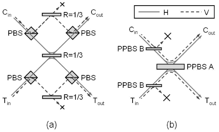
Figure 1: Schematics of the optical quantum controlled-NOT gate. (a) shows the original proposal using the two photon interaction at a beam splitter of reflectivity 1/3 and (b) shows the recently developed compact realization using partially polarizing beam splitters (PPBS).

In the context of our optical quantum controlled-NOT gate, the computational $Z$ basis and the complementary $X$ basis are defined in terms of the linear polarizations of the photons. Using the horizontal and vertical polarization states, $\mid H\rangle$ and $\mid V\rangle$, the corresponding basis states of the control qubit $C$ and the target qubit $T$ read

$$\begin{array}[]{rcccrcc}\mid 0_{Z}\rangle_{C}&=&\mid V\rangle&&\mid 0_{Z}\rangle_{T}&=&\frac{1}{\sqrt{2}}(\mid H\rangle+\mid V\rangle)\\ \mid 1_{Z}\rangle_{C}&=&\mid H\rangle&&\mid 1_{Z}\rangle_{T}&=&\frac{1}{\sqrt{2}}(\mid H\rangle-\mid V\rangle)\\ \mid 0_{X}\rangle_{C}&=&\frac{1}{\sqrt{2}}(\mid H\rangle+\mid V\rangle)&&\mid 0_{X}\rangle_{T}&=&\mid V\rangle\\ \mid 1_{X}\rangle_{C}&=&\frac{1}{\sqrt{2}}(\mid H\rangle-\mid V\rangle)&&\mid 1_{X}\rangle_{T}&=&\mid H\rangle.\end{array}$$ (17)

The ideal operation $\hat{U}_{0}$ performed by the quantum controlled-NOT in the $Z$ basis is a classical controlled-NOT gate. In the complementary $X$ basis, the roles of target and control are exchanged, and the classical operation observed is a reversed controlled-NOT gate [25]. To demonstrate the successful implementation of a quantum controlled-NOT, it is therefore sufficient to show that the device can perform both classical controlled-NOT operations.

Table 1: Measurement results for the controlled-NOT operation in the $Z$ basis (a) and the complementary reverse controlled-NOT operation in the $X$ basis (b). Bra notation defines outputs and ket notation defines inputs. Numbers in bold face are used for the fidelities of the correct gate operations.

(a)	$\langle 0_{z}0_{z}|$	$\langle 0_{z}1_{z}|$	$\langle 1_{z}0_{z}|$	$\langle 1_{z}1_{z}|$
$|0_{z}0_{z}\rangle$	0.898	0.031	0.061	0.011
$|0_{z}1_{z}\rangle$	0.021	0.885	0.006	0.088
$|1_{z}0_{z}\rangle$	0.064	0.027	0.099	0.810
$|1_{z}1_{z}\rangle$	0.031	0.096	0.819	0.054
(b)	$\langle 0_{x}0_{x}|$	$\langle 0_{x}1_{x}|$	$\langle 1_{x}0_{x}|$	$\langle 1_{x}1_{x}|$
$|0_{x}0_{x}\rangle$	0.854	0.044	0.063	0.039
$|0_{x}1_{x}\rangle$	0.013	0.099	0.013	0.874
$|1_{x}0_{x}\rangle$	0.050	0.021	0.871	0.058
$|1_{x}1_{x}\rangle$	0.019	0.870	0.040	0.071

Table 1 shows the experimental results obtained from our device, as first reported in ref. [13]. The individual output fidelities are given by the numbers in bold face. The averages of these values define the classical fidelities $F_{z}$ and $F_{x}$ according to eq.(4). We obtain $F_{z}=0.85$ and $F_{x}=0.87$. Without analyzing any further details, we can now apply eq.(12) to determine that the process fidelity of our gate must be in the range of

$$0.72\leq F_{qp}\leq 0.85.$$ (18)

Using eqs.(14) and (16), we can then show that our gate has a minimal entanglement capability $C$ and a minimal entanglement discrimination of

$$C\geq 0.44\hskip 14.22636pt\mbox{and}\hskip 14.22636ptD\geq 0.44.$$ (19)

We can therefore conclude that our gate can generate and discriminate entanglemed states, based only on the classical fidelities of local input-output relations.

7 Error Models for the Experimental Device

A more detailed analysis of our gate is possible if we include the error probabilities of the two complementary operations shown in table 1. The output errors $\eta_{x/z}(j_{x/z})$ of each classical operation can be classified according to the bit flip errors in the output, using 0 for no error, C for a control flip, T for a target flip, and B for a flip of both output bits. The averaged errors from table 1 then read

$$\eta_{z}(\mbox{C})=0.052 \eta_{x}(\mbox{C})=0.071$$

$$\eta_{z}(\mbox{T})=0.051 \eta_{x}(\mbox{T})=0.034$$

$$\eta_{z}(\mbox{B})=0.044 \eta_{x}(\mbox{B})=0.028.$$ (20)

Likewise, the error operators $\hat{F}_{i}$ can be defined by the corresponding errors in $Z$ and in $X$, using $i=\{$ 00, C0, T0, B0, 0C, CC, TC, BC, 0T, CT, TT, BT, 0B, CB, TB, BB $\}$ to define the output errors $\hat{F}_{i}=\{$ II, XI, IX, XX, ZI, YI, ZX, YX, IZ, XZ, IY, XY, ZZ, YZ, ZY, YY $\}$. Each of the six classical errors $\eta_{x/z}(j_{x/z})$ can then be identified with a sum over four diagonal elements $\chi_{ii}$ of the process matrix, as shown in table 2.

Table 2: Sum relation between experimentally observed errors and process matrix elements (*=0,C,T,B).

$\chi_{i,i}$	*0	*C	*T	*B	sum
0*	$\chi_{\mbox{\small 00,00}}$	$\chi_{\mbox{\small 0C,0C}}$	$\chi_{\mbox{\small 0T,0T}}$	$\chi_{\mbox{\small 0B,0B}}$	$0.853$
C*	$\chi_{\mbox{\small C0,C0}}$	$\chi_{\mbox{\small CC,CC}}$	$\chi_{\mbox{\small CT,CT}}$	$\chi_{\mbox{\small CB,CB}}$	$0.052$
T*	$\chi_{\mbox{\small T0,T0}}$	$\chi_{\mbox{\small TC,TC}}$	$\chi_{\mbox{\small TT,TT}}$	$\chi_{\mbox{\small TB,TB}}$	$0.051$
B*	$\chi_{\mbox{\small B0,B0}}$	$\chi_{\mbox{\small BC,BC}}$	$\chi_{\mbox{\small BT,BT}}$	$\chi_{\mbox{\small BB,BB}}$	$0.044$
sum	$0.867$	$0.071$	$0.034$	$0.028$	$1.000$

Even though it is not possible to identify the precise values of the diagonal elements, the sum rules and the positivity of the matrix elements $\chi_{ii}$ impose strong limitations on the possible error distributions. For example, the minimal process fidelity $F_{qp}$ is only obtained if all $\chi_{ii}$ representing errors in both $X$ and $Z$ are zero. The remaining diagonal elements of the process matrix are then given directly by the experimentally observed errors, as shown in table 3.

Table 3: Diagonal elements of the process matrix for the minimal process fidelity of $F_{qp}=0.72$.

$\chi_{i,i}$	*0	*C	*T	*B	sum
0*	0.720	0.071	0.034	0.028	0.853
C*	0.052	0.000	0.000	0.000	0.052
T*	0.051	0.000	0.000	0.000	0.051
B*	0.044	0.000	0.000	0.000	0.044
sum	0.867	0.071	0.034	0.028	1.000

The estimates of the diagonal elements of the process matrix can now be used to derive estimates for the fidelities of operations other than the observed controlled-NOTs in the $Z$ and $X$ basis. In particular, the available data allows more detailed predictions about processes where one qubit is in the $Z$ basis and the other is in the $X$ basis. As will be shown in the following, the correct minimal classical fidelities for these operation on the $ZX$ or $XZ$ eigenstates can in fact be determined by using the process matrix elements $\chi_{00,00}$ obtained from the minimal process fidelity estimate given in table 3.

The most simple example is the operation on $ZX$ eigenstates where the control qubit input is in a $Z$ state and the target qubit input is in an $X$ state. Since these states are eigenstates of the ideal quantum controlled-NOT operator $U_{0}$, the ideal gate performs the identity operation on these $ZX$ inputs. We can now estimate the minimal fidelity of this identity operation from table 1 by identifying the output errors that preserve $ZX$, $\hat{F}_{i}=\{II,ZI,IX,ZX\}$. The classical fidelity $F_{I}$ of the identity operation is therefore given by

$$F_{I}=\chi_{\mbox{00,00}}+\chi_{\mbox{0C,0C}}+\chi_{\mbox{T0,T0}}+\chi_{\mbox{TC,TC}}.$$ (21)

This fidelity can be minimized by associating the errors $\eta_{z}(\mbox{C})$ with $\chi_{\mbox{\small C0,C0}}$, $\eta_{z}(\mbox{B})$ with $\chi_{\mbox{\small B0,B0}}$, $\eta_{x}(\mbox{T})$ with $\chi_{\mbox{\small 0T,0T}}$, and $\eta_{x}(\mbox{B})$ with $\chi_{\mbox{\small 0B,0B}}$. The errors changing the control qubit in $Z$ and the target bit in $X$ then contribute separately to the total errors in the identity operation on $ZX$ states, and the minimal fidelity is given by

$$F_{I}\geq 1-(\eta_{z}(\mbox{C})+\eta_{z}(\mbox{B})+\eta_{x}(\mbox{T})+\eta_{x}(\mbox{B}))=0.842.$$ (22)

As mentioned above, this result is consistent with the distribution of process matrix elements shown in table 3, indicating that the assumption of a minimal process fidelity of $F_{qp}=F_{Z}+F_{X}-1$ also implies a minimal fidelity $F_{I}$ for the identity operation.

Next, we can analyze the entanglement generation from inputs in $XZ$ eigenstates. The ideal operation $\hat{U}_{0}$ generates maximally entangled two qubit Bell states from each of the possible $XZ$ inputs. We can therefore derive an estimate of the entanglement capability $C$ from the fidelity $F_{C}$ of this operation. Again, we first identify the errors output errors that preserve the output states. In this case, these errors are $\hat{F}_{i}=\{II,XX,YY,ZZ\}$, corresponding to an entanglement generation fidelity of

$$F_{C}=\chi_{\mbox{00,00}}+\chi_{\mbox{B0,B0}}+\chi_{\mbox{BB,BB}}+\chi_{\mbox{0B,0B}}.$$ (23)

Like the fidelity $F_{I}$ of the identity operation, this fidelity is also minimal for the error distribution shown in table 3. Specifically,

$$F_{C}\geq 1-(\eta_{z}(\mbox{C})+\eta_{z}(\mbox{T})+\eta_{x}(\mbox{C})+\eta_{x}(\mbox{T}))=0.792.$$ (24)

We therefore obtain an improved estimate of the entanglement capability of our gate,

$$C\geq 2F_{C}-1\geq 0.584.$$ (25)

The more detailed analysis of the error distribution has thus provided us with additional information on the entanglement capability of our experimental device.

Finally, we can also improve our estimate of the entanglement discrimination $D$ by considering the fidelity $F_{D}$ of the operation that converts Bell state inputs into local $XZ$ eigenstates. In this case, the errors that preserve the correct output states are $\hat{F}_{i}=\{II,XI,IZ,XZ\}$, corresponding to a Bell analyzer fidelity of

$$F_{D}=\chi_{\mbox{00,00}}+\chi_{\mbox{C0,C0}}+\chi_{\mbox{0T,0T}}+\chi_{\mbox{CT,CT}}.$$ (26)

Again, the minimal fidelity can be obtained using the diagonal matrix elements shown in table 3, and the corresponding minimal fidelity estimate is given by

$$F_{D}\geq 1-(\eta_{z}(\mbox{T})+\eta_{z}(\mbox{B})+\eta_{x}(\mbox{C})+\eta_{x}(\mbox{B}))=0.806.$$ (27)

Interestingly, this fidelity is a little bit higher than the fidelity $F_{C}$ for entanglement generation. We therefore obtain a minimal entanglement discrimination $D$ that exceeds the minimal entanglement capability $C$ obtained from the same data,

$$D\geq 2F_{D}-1\geq 0.612.$$ (28)

The error analysis of the local $Z$ and $X$ operations thus shows that our gate can successfully generate and distinguish entangled states, with somewhat stronger evidence for the reliability of Bell state discrimination.

8 Conclusions

As the analysis of the errors in our experimental quantum controlled-NOT gate has shown, the classical logic operations observed in a pair of complementary basis sets can provide surprisingly detailed information about the performance of a quantum device. In particular, it is possible to obtain good estimates of the process fidelity $F_{qp}$, the entanglement capability $C$, and the entanglement discrimination $D$ from only a small fraction of the data needed for a complete reconstruction of the process matrix by quantum process tomography. Interestingly, the complementary processes of the quantum controlled-NOT are completely local. It is therefore possible to estimate the non-local properties of the gate described by the entanglement capability $C$ and the entanglement discrimination $D$ without ever generating entangled states.

Besides the obvious advantages of gaining quick and efficient access to the most important measures characterizing a quantum process, the analysis of the process matrix in terms of its observable effects also allows us to take a peek inside the ”black box” that is postulated in so many approaches to quantum computation. In particular, it is possible to identify the features of quantum coherence and entanglement more directly with the experimentally accessible data by identifying mathematical expansions that fit the specific features of the quantum process under investigation. Hopefully, this is only a first step towards a better understanding of the still somewhat mysterious nature of quantum information processes.

References

- [1] M.A. Nielsen and I.L. Chuang, Quantum Computation and Quantum Information (Cambridge University Press, 2000), chapter 4.
- [2] Q.A. Turchette, C.J. Hood, W. Lange, H. Mabuchi, and H. J. Kimble, Phys. Rev. Lett 75, 4710 (1995).
- [3] C. Monroe, D.M. Meekhof, B.E. King, W.M. Itano, and D.J. Wineland, Phys. Rev. Lett. 75, 4714 (1995).
- [4] Y.A. Pashkin, T. Yamamoto, O. Astafiev, Y. Nakamura, D.V. Averin, and J.S. Tsai, Nature (London) 421, 823 (2003).
- [5] F. Schmidt-Kaler, H. Häffner, M. Riebe, S. Gulde, G. P. T. Lancaster, T. Deuschle, C. Becher, C.F. Roos, J. Eschner, and R. Blatt, Nature (London) 422, 408 (2003).
- [6] D. Leibfried, B. DeMarco, V. Meyer, D. Lucas, M. Barret, J. Britton, W.M. Itano, B. Jelenkovic, C. Langer, T. Rosenband, and D.J. Wineland, Nature (London) 422, 412 (2003).
- [7] T. B. Pittman, M. J. Fitch, B. C Jacobs, and J. D. Franson, Phys Rev. A 68, 032316 (2003).
- [8] J.L. O‘Brien, G.J. Pryde, A.G. White, T.C. Ralph, and D. Branning, Nature (London) 426, 264 (2003).
- [9] Y.-F. Huang, X.-F. Ren, Y.-S. Zhang, L.-M. Duan, and G.-C. Guo, Phys. Rev. Lett. 93, 240501 (2004).
- [10] Z. Zhao, A.-N. Zhang, Y.-A. Chen, H. Zhang, J.-F. Du, T. Yang, and J.-W. Pan, Phys. Rev. Lett. 94, 030501 (2005).
- [11] N. K. Langford, T. J. Weinhold, R. Prevedel, K. J. Resch, A. Gilchrist, J. L. O’Brien, G. J. Pryde, and A. G. White, Rev. Lett. 95, 210504 (2005).
- [12] N. Kiesel, C. Schmid, U. Weber, R. Ursin, and H. Weinfurter, Phys. Rev. Lett. 95, 210505 (2005).
- [13] R. Okamoto, H. F. Hofmann, S. Takeuchi, and K. Sasaki, Phys. Rev. Lett. 95, 210506 (2005).
- [14] H.F. Hofmann, Phys. Rev. Lett. 94, 160504 (2005).
- [15] M.A. Nielsen and I.L. Chuang, Quantum Computation and Quantum Information (Cambridge University Press, 2000), chapter 8.
- [16] G. Mahler and V. A. Weberruß, Quantum Networks (Springer, 1998), chapter 2.
- [17] M. Horodecki, P. Horodecki, and R. Horodecki, Phys. Rev. A 60, 1888, (1999).
- [18] J.F. Poyatos, J.I. Cirac, and P. Zoller, Phys. Rev. Lett.78, 390 (1997).
- [19] M. Horodecki P. Horodecki, and R. Horodecki, Phys. Lett. A 223, 1 (1996).
- [20] B. M. Terhal, Phys. Lett. A 271, 319 (2000).
- [21] M. Lewenstein, B. Kraus, J. I. Cirac, and P. Horodecki, Phys. Rev. A 62, 052310 (2000).
- [22] G. Toth and O. Gühne, Phys. Rev. Lett. 94, 060501 (2005).
- [23] H.F. Hofmann, and S. Takeuchi, Phys. Rev. A 66, 024308 (2002).
- [24] T.C. Ralph, N.K. Langford, T.B. Bell, and A.G. White, Phys. Rev. A 65, 062324 (2002).
- [25] H.F. Hofmann, Phys. Rev. A 72, 022329, (2005).