Symmetries and noise in quantum walk

Abstract

We study some discrete symmetries of unbiased (Hadamard) and biased quantum walk on a line, which are shown to hold even when the quantum walker is subjected to environmental effects. The noise models considered in order to account for these effects are the phase flip, bit flip and generalized amplitude damping channels. The numerical solutions are obtained by evolving the density matrix, but the persistence of the symmetries in the presence of noise is proved using the quantum trajectories approach. We also briefly extend these studies to quantum walk on a cycle. These investigations can be relevant to the implementation of quantum walks in various known physical systems. We discuss the implementation in the case of NMR quantum information processor and ultra cold atoms.

I Introduction

Random walk, which has found applications in many fields barber-ninham ; chandra , is an important constituent of information theory. It has played a very prominent role in classical computation. Markov chain simulation, which has emerged as a powerful algorithmic tool mark , as well as many other classical algorithms, are based on random walks. Quantum random walks aharonov , the generalization of classical random walks to situations where the quantum uncertainties play a predominant role, are of both mathematical and experimental interest and have been investigated by a number of groups. It is believed that exploring quantum random walks kempe allows, in a similar way, a search for new quantum algorithms, a few of which have already been proposed childs ; shenvi ; childs1 ; ambainis . Experimental implementation of the quantum walk has also been reported ryan ; du . Various other schemes have been proposed for the physical realization of the quantum walks travaglione ; rauss ; eckert ; chandra06 ; ma .

The evolution of a discrete classical random walk, involving steps of a given length, is described in terms of probabilities. On the other hand, the evolution of a discrete quantum random walk is described in terms of probability amplitudes. An unbiased one dimensional classical random walk with the particle initially at $x_{0}$ evolves in such a way that at each step, the particle moves with probability 1/2 one step to the left or right. In a quantum mechanical analog the state of the particle evolves at each step into a coherent superposition of moving one step to the right and one step to the left.

In the one dimensional quantum (Hadamard) walk the particle initially prepared in a product state of the coin (internal) and position (external) degree of freedom, is subjected to a rotation in the coin Hilbert space, followed by a conditional shift operation, to evolve it into a superposition in the position space. The process is iterated without resorting to intermediate measurements to realize a large number of steps of quantum walk, before a final measurement.

A one dimensional quantum (Hadamard) walk starting from initial state $|0\rangle\otimes|x_{0}\rangle$ or $|1\rangle\otimes|x_{0}\rangle$ (where the first register refers to the coin degree of freedom, and the second register to the external, spatial degree of freedom) induces an asymmetric probability distribution of finding the particle after $N$ number of steps of quantum walk. A particle with initial coin state $|0\rangle$ drifts to the right (solid line in Figure 1) and particle with initial state $|1\rangle$ drifts to the left (dashed line in Figure 1). This asymmetry arises from the fact that the Hadamard coin treats the two directions $|0\rangle$ and $|1\rangle$ differently; it multiplies the phase by -1 only in case of $|0\rangle$. It follows that to obtain left-right symmetry, one needs to start the coin in the state $|0\rangle+i|1\rangle$ (Figure 2).

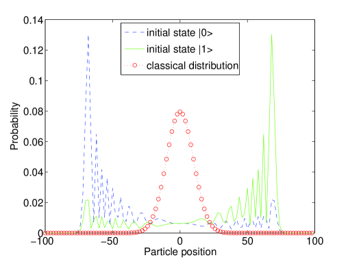
Figure 1: (color online) Probability distribution of the quantum walk with the initial state $|0\rangle$ (solid line) and initial state $|1\rangle$ (dashed line) on the position. The distribution is for 100 steps.

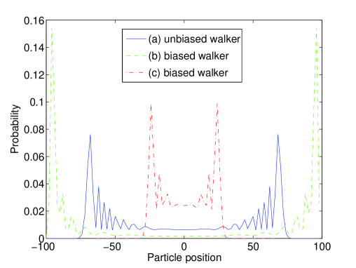
Figure 2: (color online) The probability distribution of an unbiased walker, and a biased quantum walker using an SU(2) operator of the form (6) as the quantum coin toss. (a) Unbiased quantum walker ($\theta=45^{\circ}$); (b) Biased quantum walker with $\theta=15^{\circ}$; (c) Biased quantum walker with $\theta=75^{\circ}$. The distribution is for 100 steps.

In this paper we report that the quantum walk– both the unbiased (Hadamard) as well as the biased– remains invariant under certain operations, i.e., the probability distribution of the walker’s position remains unchanged under the inclusion of these operations at each step of the walk. We refer to these discrete operations as symmetries of the quantum walk. We further study these symmetries in the presence of environmental effects, modeled by various noise channels. These results were obtained by numerical integration rather than simulation. We extend these studies to quantum walk on a cycle, which can be conveniently generalized to more general graphs. It is shown that the above symmetries do not hold, in general, for a quantum walk on a cycle and hence for the closed graph, but leads to other interesting behavior. These observations can have important implications for a better insight into, and for simplifying certain implementations of, quantum walks.

This paper is organized as follows. Section II briefly recapitulates the theory of quantum random walk. Section III discusses quantum walk augmented by various symmetry operations, both in the case of a biased and unbiased quantum coin. The above observations are generalized to the case of a noisy quantum walk in Section IV, with Section IV.1 treating noise as phase-flip and bit-flip channels, and Section IV.2 treating noise as a generalized amplitude damping channel. Whereas the numerical results presented here, involve evolving the density operator of the system, we have found it convenient to explain the symmetries using quantum trajectories. In Section V we extend these studies to the quantum walk on the cycle which can be generalzed to all closed graphs in general. In Section VI we show that the application of these ideas can help simplify certain experimental implementations of quantum walk. We also discuss the physical systems, NMR quantum-information processor and ultracold atoms, where the results presented in this article can be applied. In Section VII, we make our conclusions.

II Quantum random walk

Unlike classical random walk, two degrees of freedom are required for quantum random walks, the internal, coin degree of freedom, represented by the two-dimensional Hilbert space $\mathcal{H}_{c}$, spanned by the basis states $|0\rangle$ and $|1\rangle$, and the particle degree of freedom, represented by the position Hilbert space $\mathcal{H}_{p}$, spanned by basis states $|x\rangle$, $x\in\mathbb{Z}$. The state of the total system is in the space $\mathcal{H}=\mathcal{H}_{c}\otimes\mathcal{H}_{p}$. The internal state of the particle determines the direction of the particle’s movement when the conditional unitary shift operator $U$ is applied on the particle, whose initial state is given by a product state, for example, $|\Psi_{in}\rangle=\frac{1}{\sqrt{2}}[|0\rangle+|1\rangle]\otimes|\Psi_{x_{0}}\rangle$, where

$$U = |0\rangle\langle 0|\otimes\sum_{x\in\mathbb{Z}}|x-1\rangle\langle x|+|1\rangle\langle 1|\otimes\sum_{x\in\mathbb{Z}}|x+1\rangle\langle x|$$ (1)

$$\equiv |0\rangle\langle 0|\otimes\hat{A}+|1\rangle\langle 1|\otimes\hat{A}^{{\dagger}}.$$

Here $\hat{A}$ and $\hat{A}^{{\dagger}}$ are unitary operators that are notationally reminiscent of annihilation and creation operations, respectively. The conditional shift can also be written as

$$U=\exp(-2iS_{z}\otimes Pl),$$ (2)

$P$, being the momentum operator and $S_{z}$, the operator corresponding to the step of length $l$.

Conditioned on the internal state being $|0\rangle$ ($|1\rangle$), the particle moves to the left (right), i.e., $U|0\rangle\otimes|x\rangle=|0\rangle\otimes|x-1\rangle$ and $U|1\rangle\otimes|x\rangle=|1\rangle\otimes|x+1\rangle$. Application of $U$ on $|\Psi_{in}\rangle$ spatially entangles the $\mathcal{H}_{c}$ and $\mathcal{H}_{p}$ and implements quantum (Hadamard) walk,

$$U|\Psi_{in}\rangle=\frac{1}{\sqrt{2}}[|0\rangle\otimes e^{-iPl}+|1\rangle\otimes e^{iPl}]|\Psi_{x_{0}}\rangle.$$ (3)

Each step of the quantum (Hadamard) walk is composed of a Hadamard operation (rotation) $H$,

$$H=\frac{1}{\sqrt{2}}\left(\begin{array}[]{clcr}1&&1\\ 1&&-1\end{array}\right),$$ (4)

on the particle, bringing them to a superposition state with equal probability, such that,

$$(H\otimes\mathbbm{1})|0,x\rangle = \frac{1}{\sqrt{2}}[|0,x\rangle+|1,x\rangle],$$

$$(H\otimes\mathbbm{1})|1,x\rangle = \frac{1}{\sqrt{2}}[|0,x\rangle-|1,x\rangle],$$ (5)

and, a subsequent unitary conditional shift operation, $U$, which moves the particle into an entangled state in the position space.

The probability amplitude distribution arising from the iterated application of $W=U(H\otimes\mathbbm{1})$ is significantly different from the distribution of the classical walk after the first two steps kempe . If the coin initially is in a suitable superposition of $|0\rangle$ and $|1\rangle$ then the probability amplitude distribution after $n$ steps of quantum walk will have two maxima symmetrically displaced from the starting point. The variance of quantum version is known to grow quadratically with number of steps $n$, $\sigma^{2}\propto n^{2}$ compared to the linear growth, $\sigma^{2}\propto n$ for the classical walk.

Figure 2 shows the probability distribution of finding the position of the quantum walker using a biased walker with $\theta=15^{\circ}$ and $\theta=75^{\circ}$, respectively, using a general $SU(2)$ operator of the form,

$$B(\xi,\theta,\zeta)=\left(\begin{array}[]{clcr}e^{i\xi}\cos(\theta)&&e^{i\zeta}\sin(\theta)\\ e^{-i\zeta}\sin(\theta)&&-e^{-i\xi}\cos(\theta)\end{array}\right),$$ (6)

where we have set $\xi=\zeta=0$. Note that $H=B(0,45^{\circ},0)$. Replacing the Hadamard coin with an arbitrary $SU(2)$ operator yields a biased coin toss, with $\theta<45^{\circ}$ or $\theta>45^{\circ}$. The value of $\sigma$ can be increased or decreased, respectively.

III Bit flip and phase flip symmetries in quantum walk

Consider the application of the modified conditional shift operator $U^{\prime}=|1\rangle\langle 0|\otimes\hat{A}+|0\rangle\langle 1|\otimes\hat{A}^{{\dagger}}$ instead of Eq. (1). In place of Eq. (2), one has:

$$U^{\prime}=(X\otimes\mathbb{I})\exp(-2iS_{z}\otimes Pl),$$ (7)

where $X$ is the Pauli $X$ operator. Since $U^{\prime}=XU$, i.e., it is equivalent to an application of bit flip following $U$, conditioned on the internal state being $|0\rangle$ ($|1\rangle$), the particle will move to the left (right) and changes its internal state to $|1\rangle$ ($|0\rangle$). Thus, $U^{\prime}|0\rangle\otimes|x\rangle=|1\rangle\otimes|x-1\rangle$ and $U^{\prime}|1\rangle\otimes|x\rangle=|0\rangle\otimes|x+1\rangle$.

A relevant observation in this context is that there are physical systems where the implementation of $U^{\prime}$ is easier than that of $U$ chandra06 . In that case, applying a compensatory bit flip on the internal state, after each application of $U^{\prime}$, reduces the modified quantum walk to the usual scheme. In all this would require $(n-1)$ compensatory bit flips, which adds to the complexity of the experimental realization. However, this additional complexity can be eliminated. For an unbiased quantum walk, applying a bit flip in each step can be shown to be equivalent to a spatial inversion of the position probability distribution. A quick way to see why bit flips (for an unbiased quantum walk) are harmless is to note that they are also equivalent to relabeling the edges of the graph on which the quantum walk takes place, so that each end of each edge has the same label ken05 . (It is worth noting that in Ref. rauss , bit flips are employed to improve the practical implementation of a quantum walk of atoms in an optical lattice.) We may in this sense call a bit flip together with spatial inversion a symmetry of the unbiased quantum walk on a line. To be specific, a quantum walk symmetry is any unitary operation which may uniformly augment each step of a quantum walk without affecting the position probability distribution. Experimentally, the symmetries are useful in identifying variants of a given quantum walk protocol that are equivalent to it. This motivates us to look for other (discrete) symmetries of the quantum walk, which we study below. We begin with Theorem 1, where we note four discrete symmetries, associated with the matrices $B^{(j)}$ $(j=1,2,3,4)$ (cf. Eq. (17)), of the quantum walk. Thereafter two of these symmetries, $B^{(1)}$ and $B^{(2)}$, are identified with operations that are relevant from the perspective of physical implementation. It is an interesting open question of relevance to practical implementation of quantum walks, whether other such symmetries of the quantum walk exist.

Theorem 1

If $B$ in Eq. (6) is replaced by any of $B^{(1)}$, $B^{(2)}$, $B^{(3)}$, or $B^{(4)}$, given by,

$$B^{(1)}\equiv\left(\begin{array}[]{clcr}e^{i\xi}\cos(\theta)&&e^{i\zeta}\sin(\theta)\\ e^{i(\phi-\zeta)}\sin(\theta)&&-e^{i(\phi-\xi)}\cos(\theta)\end{array}\right),\hskip 11.38092pt B^{(2)}\equiv\left(\begin{array}[]{clcr}e^{i\xi}\cos(\theta)&&e^{i(\phi+\zeta)}\sin(\theta)\\ e^{-i\zeta}\sin(\theta)&&-e^{i(\phi-\xi)}\cos(\theta)\end{array}\right),$$ (12)

$$B^{(3)}\equiv\left(\begin{array}[]{clcr}e^{i(\phi+\xi)}\cos(\theta)&&e^{i(\phi+\zeta)}\sin(\theta)\\ e^{-i\zeta}\sin(\theta)&&-e^{-i\xi}\cos(\theta)\end{array}\right),\hskip 11.38092pt B^{(4)}\equiv\left(\begin{array}[]{clcr}e^{i(\phi+\xi)}\cos(\theta)&&e^{i\zeta}\sin(\theta)\\ e^{i(\phi-\zeta)}\sin(\theta)&&-e^{-i\xi}\cos(\theta)\end{array}\right),$$ (17)

the resulting position probability distribution of the quantum walk remains unchanged.

Proof. With the notation $B\equiv\{b_{j,k}\}$ and $B^{(j)}\equiv\{b^{(j)}_{j,k}\}$, we find $b^{(1)}_{jk}=b_{jk}e^{ij\phi}$, $b^{(2)}_{jk}=b_{jk}e^{ik\phi}$, $b^{(3)}_{jk}=b_{jk}e^{i\bar{j}\phi}$, $b^{(4)}_{jk}=b_{jk}e^{i\bar{k}\phi}$, where the matrix indices $j,k$ take values 0 and 1, $i\equiv+\sqrt{-1}$, and the overbar denotes a NOT operation ($0\leftrightarrow 1$). The state vector obtained, after $n$ steps, using $B$ and $B^{(1)}$ as the coin rotation operations, are, respectively, given by

$$|\Psi_{1}\rangle = (UB)^{n}|\alpha,\beta\rangle=\sum_{j_{1},j_{2},\cdots,j_{n}}b_{j_{n},j_{n-1}}\cdots b_{j_{2},j_{1}}b_{j_{1},\alpha}|j_{n},\beta+2J-n\rangle,$$

$$|\Psi_{2}\rangle = (UB^{(1)})^{n}|\alpha,\beta\rangle=\sum_{j_{1},j_{2},\cdots,j_{n}}b_{j_{n},j_{n-1}}\cdots b_{j_{2},j_{1}}b_{j_{1},\alpha}(e^{i\phi})^{j_{n-1}+\cdots+j_{1}+\alpha}|j_{n},\beta+2J-n\rangle,$$ (18)

where $J=j_{1}+\cdots+j_{n}$. Consider an arbitrary state $|a,b\rangle$ in the computational-and-position basis. Now, $\langle a,b|\Psi_{1}\rangle=e^{i\eta\phi}\langle a,b|\Psi_{2}\rangle$, where $\eta=j_{n-1}+\cdots+j_{1}+\alpha$, which is fixed for given $\alpha$ and $b$, and determined by $b=\beta+2J-n$ and $j_{n}=a$. As a result, $|\langle a,b|\Psi_{1}\rangle|^{2}+|\langle\bar{a},b|\Psi_{1}\rangle|^{2}=|\langle a,b|\Psi_{2}\rangle|^{2}+|\langle\bar{a},b|\Psi_{2}\rangle|^{2}$. A similar proof of invariance of the position distribution can be demonstrated to hold when $B$ is replaced by one of the other $B^{(j)}$’s $(j=2,3,4)$. On account of the linearity of quantum mechanics, the invariance of the walk statistics under exchange of the $B^{(j)}$’s and $B$ holds even when the initial state $|\alpha,\beta\rangle$ is replaced by a general superposition or a mixed state. $\blacksquare$

Interchanging $B$ and the $B^{(j)}$’s may be considered as a discrete symmetry operation $G:B\rightarrow B^{\star}$ (where $B^{\star}$ denotes any of the $B^{(j)}$’s in Eq. (17)), that leaves the positional probability distribution invariant. We express this by the statement that

$$\widehat{W}\simeq{\bf G}\widehat{W},$$ (19)

where ${\bf G}$ refers to the application of $G$ at each step of the walk, and $\widehat{W}$ refers to the walk operation of evolving the initial state through $n$ steps and then measuring in the position basis. Knowledge of this symmetry can help simplify practical quantum walks. Below we identify two of these quantum walk symmetry operations $B\leftrightarrow B^{(1)}$ and $B\leftrightarrow B^{(2)}$, associated with physical operations of interest.

We first consider the phase shift gate $\Phi(\phi)\equiv|0\rangle\langle 0|+e^{i\phi}|1\rangle\langle 1|$ as a symmetry operation of a quantum walk. In our model, the quantum operation for each step is augmented by the insertion of $\Phi(\phi)$ just after the operation $UB$. At each step, the walker evolves according to:

$$U_{\Phi} \equiv \left(\begin{array}[]{ll}1&0\\ 0&e^{i\phi}\end{array}\right)\left[\left(\begin{array}[]{lcl}1&{}{}\hfil&0\\ 0&&0\end{array}\right)\otimes\hat{A}+\left(\begin{array}[]{lcl}0&&0\\ 0&&1\end{array}\right)\otimes\hat{A}^{{\dagger}}\right]\left(\begin{array}[]{clcr}e^{i\xi}\cos(\theta)&{}{}&e^{i\zeta}\sin(\theta)\\ e^{-i\zeta}\sin(\theta)&&-e^{-i\xi}\cos(\theta)\end{array}\right)$$ (28)

$$= \left[\left(\begin{array}[]{lcl}1&{}{}\hfil&0\\ 0&&0\end{array}\right)\otimes\hat{A}+\left(\begin{array}[]{lcl}0&&0\\ 0&&1\end{array}\right)\otimes\hat{A}^{{\dagger}}\right]\left(\begin{array}[]{clcr}e^{i\xi}\cos(\theta)&{}{}&e^{i\zeta}\sin(\theta)\\ e^{i(\phi-\zeta)}\sin(\theta)&&-e^{i(\phi-\xi)}\cos(\theta)\end{array}\right).$$ (35)

This is equivalent to replacing $B$ by $B^{(1)}$, which, according to Theorem 1, leaves the walker distribution invariant. Thus the operation $\Phi(\phi)$, applied at each step, is a symmetry of the quantum walk.

As a special case, the phase flip operation ($Z$) applied at each step, obtained by setting $\phi=\pi$, is a symmetry of the quantum walk. Representing the inclusion of operations $\Phi$ or $Z$ at each step of the walk by ${\bf\Phi}$ or ${\bf Z}$, respectively, we express this symmetry by the statements:

$$\widehat{W}\simeq{\bf\Phi}\widehat{W},$$ (36a)

$$\widehat{W}\simeq{\bf Z}\widehat{W}.$$ (36b)

Unlike the phase flip operation, bit flip is not a symmetry of the quantum walk on a line. However, the combined application of bit flip along with angular reflection $R$ ($\theta\rightarrow\pi/2-\theta$, i.e., $\sin\theta\leftrightarrow\cos\theta$, and $\xi\leftrightarrow-\zeta$) and parity $P$ ($\hat{A}\leftrightarrow\hat{A}^{{\dagger}}$) turns out to be a symmetry operation. These three operations commute with each other. By the inclusion of $PRX$, the walker evolves by $([PRX]UB)^{n}$. At each step, the walker evolves according to:

$$U_{P} \equiv PR\left(\begin{array}[]{ll}0&1\\ 1&0\end{array}\right)\left[\left(\begin{array}[]{lcl}1&{}{}\hfil&0\\ 0&&0\end{array}\right)\otimes\hat{A}+\left(\begin{array}[]{lcl}0&&0\\ 0&&1\end{array}\right)\otimes\hat{A}^{{\dagger}}\right]\left(\begin{array}[]{clcr}e^{i\xi}\cos(\theta)&{}{}&e^{i\zeta}\sin(\theta)\\ e^{-i\zeta}\sin(\theta)&&-e^{-i\xi}\cos(\theta)\end{array}\right)$$ (45)

$$= \left[\left(\begin{array}[]{lcl}1&{}{}\hfil&0\\ 0&&0\end{array}\right)\otimes\hat{A}+\left(\begin{array}[]{lcl}0&&0\\ 0&&1\end{array}\right)\otimes\hat{A}^{{\dagger}}\right]\left(\begin{array}[]{clcr}e^{i\xi}\cos(\theta)&{}{}&-e^{i\zeta}\sin(\theta)\\ e^{-i\zeta}\sin(\theta)&&e^{-i\xi}\cos(\theta)\end{array}\right).$$ (52)

This is equivalent to replacing $B$ by $B^{(2)}$ with $\phi=\pi$, which, according to Theorem 1, should leave the walker distribution invariant. Thus the operation $PRX$ applied at each step, is a symmetry of the quantum walk. It will be convenient henceforth to choose $\xi=\zeta=0$, so that $R$ will simply correspond to the replacement $\theta\rightarrow\pi/2-\theta$.

Representing the inclusion of operations $P$, $R$ or $X$ at each step of the walk by ${\bf P}$, ${\bf R}$ or ${\bf X}$, respectively, we express this symmetry by the statements:

$$\widehat{W} \simeq {\bf PRX}\widehat{W},$$ (53a)

$${\bf X}\widehat{W} \simeq {\bf PR}\widehat{W}.$$ (53b)

Eq. (53a) was proved immediately above. Eq. (53b) follows from Eq. (53a), since the operations ${\bf P}$, ${\bf R}$ and ${\bf X}$ mutually commute, and $X^{2}=\mathbb{I}$. It expresses that fact that applying the $X$ operation at each step is equivalent to replacing a quantum walk by its angle-reflected, spatially inverted counterpart. The observation made at the beginning of this Section pertains to the special case of $\theta=45^{\circ}$. By a similar technique the following symmetries may be proved:

$${\bf X}\widehat{W}~{}\simeq~{}{\bf XZ}\widehat{W}~{}\simeq~{}{\bf ZX}\widehat{W}.$$ (54)

The first equivalence easily follows from Eq. (36).

IV Environmental effects

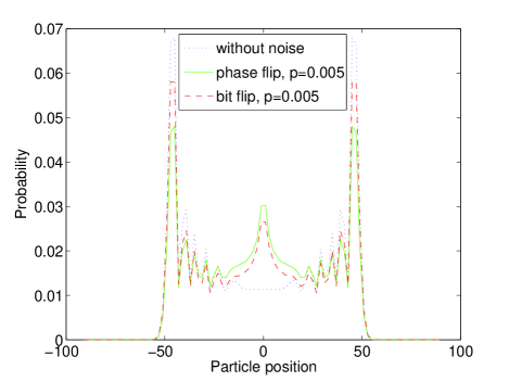
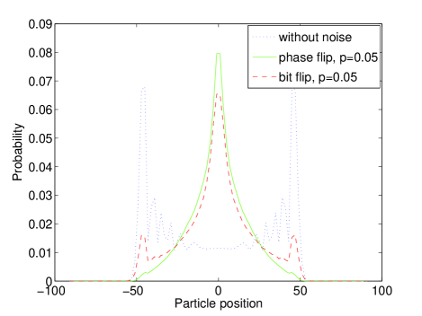
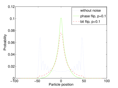
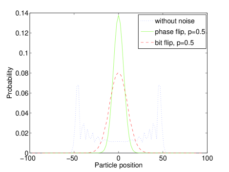
Figure 3: (color online) The effect of environmental decoherence on the position probability distribution of a biased quantum walker subjected to a noisy channel. Coin bias is of the form Eq. (6) with $\theta=60^{\circ}$. The noise is modelled as a phase flip (solid line) or bit flip (dashed line) channel, characterized by Eqs. (57) and (62), respectively, at various noise levels $p$: (a) $p=0.005$ (b) $p=0.05$; (c) $p=0.1$; (d) $p=0.5$, which corresponds to a fully classical random walk. Comparing Figure (d) with Figure 4(d), we note that the distribution in the case of maximal bit flip noise is the same.

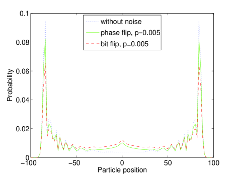
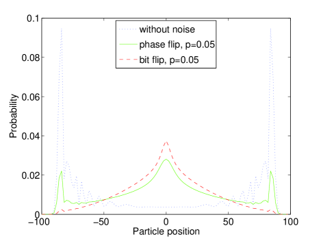
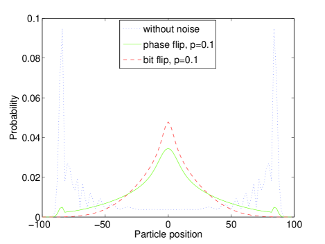
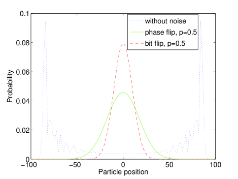
Figure 4: (color online) The effect of environmental decoherence on the position probability distribution of a biased quantum walker subjected to a noisy channel. Coin bias is of the form Eq. (6) with $\theta=30^{\circ}$. The noise is modelled as a phase flip (solid line) or bit flip (dashed line) channel, characterized by Eqs. (57) and (62), respectively, at various noise levels $p$: (a) $p=0.005$ (b) $p=0.05$; (c) $p=0.1$; (d) $p=0.5$, which corresponds to a fully classical random walk.

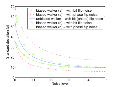
Figure 5: (color online) Variation of standard deviation with noise level, for both phase noise and bit flip noise. Solid line is for an unbiased walker. For biased walker (a) $\theta=30^{\circ}$ and (b) $\theta=60^{\circ}$. In the classical limit of $p=0.5$, the standard deviation converges to a fixed value for bit flip noise, irrespective of $\theta$, but different for phase flip noise. The convergence happens because, at maximum bit flip noise ($p=0.5$), the measurement outcome in the computational basis is completely randomized, and the presence or absence of bias is irrelevant. On the other hand, the non-convergence in the case of phase flip noise is due to the fact that the asymptotic mixed state obtained via a phase damping channel depends on the initial state parameter $\theta$.

A quantum walk implemented on a quantum computer is inevitably affected by errors caused by noise due to the environment. We consider three physically relevant models of noise: a phase flip channel (which is equivalent to a phase damping or purely dephasing channel), a bit flip channel and a generalized amplitude damping channel ($T\geq 0$). In all cases, our numerical implementation of these channels evolves the density matrix employing the Kraus operator representation for them. However to explain symmetry effects, it is convenient to use the quantum trajectories approach, discussed below.

IV.1 Decoherence via phase damping and bit flip channels

In studying the status of the walk symmetries in the presence of noise, it is advantageous to employ the quantum trajectories approach bru02 . This simplifies the description of an open quantum system in terms of a stochastically evolving pure state, which allows us to adapt the symmetry results for the pure states, given in the preceding section, to mixed states.

We call the sequence of walk step operations $\widehat{X}\equiv(UB_{n})(UB_{n-1})\cdots(UB_{1})$ a ‘quantum trajectory’. (More precisely, a trajectory refers to the sequence of states produced by these operations, for which the above serves as a convenient representation.) If all the $B_{j}$’s are the same, then $\widehat{X}$ is the usual ‘homogeneous’ quantum walk $\widehat{W}$. In general, the $B_{j}$’s may be different $SU(2)$ operators, corresponding to a varying bias in the coin degree of freedom. More generally, each step of the walk may include generalized measurements whose outcomes are known (Section IV.2). If each walk step in $\widehat{X}$ is subjected to a fixed symmetry operation $G$, the result is a new quantum trajectory ${\bf G}\widehat{X}\equiv(UB_{n}^{\star})(UB_{n-1}^{\star})\cdots(UB_{1}^{\star})$. We have the following generalization of Theorem 1 to inhomogeneous quantum walks on a line.

Theorem 2

Given any quantum walk trajectory $\widehat{X}=(UB_{n})\cdots(UB_{1})$, the symmetry ${\cal G}$ holds, i.e., $\widehat{X}\simeq{\bf G}\widehat{X}$. If the operation ${\bf\Phi}$ is restricted to ${\bf Z}$, then the symmetries hold even when some of the $U$’s are replaced by $U^{{\dagger}}$’s.

Proof. In the proof of Theorem 1, we note that if, in each step of the walk, we alter the rotation $B$ by the transformation $G$, the proof still goes through. That is, $|\Psi_{1}\rangle\equiv(UB_{n})(UB_{n-1})\cdots(UB_{1})|\alpha,\beta\rangle$ and $|\Psi_{2}\rangle\equiv(UB_{n}^{\star})(UB_{n-1}^{\star})\cdots(UB_{1}^{\star})|\alpha,\beta\rangle$ produce the same position distribution.

Suppose that in some of the walk steps, $U$ is replaced with $U^{{\dagger}}$. In place of Eq. (III), we have

$$|\Psi_{1}\rangle = (UB_{n})\cdots(U^{{\dagger}}B_{j})\cdots(UB_{1})|\alpha,\beta\rangle$$ (55a)

$$= \sum_{j_{1},j_{2},\cdots,j_{n}}b_{j_{n},j_{n-1}}\cdots b_{j_{2},j_{1}}b_{j_{1},\alpha}|j_{n},\beta+2(J_{1}-J_{2})-(n_{1}-n_{2})\rangle,$$

$$|\Psi_{2}\rangle = (UB_{n}^{(1)})\cdots(U^{{\dagger}}B_{j}^{(1)})\cdots(UB_{1}^{(1)})|\alpha,\beta\rangle$$ (55b)

$$= \sum_{j_{1},j_{2},\cdots,j_{n}}b_{j_{n},j_{n-1}}\cdots b_{j_{2},j_{1}}b_{j_{1},\alpha}(-1)^{j_{n-1}+\cdots+j_{1}+\alpha}|j_{n},\beta+2(J_{1}-J_{2})-(n_{1}-n_{2})\rangle,$$

where $J_{1}=\sum_{k}j_{k}$ for the $n_{1}$ steps $k$ where operator $U$ is used, and $J_{2}=\sum_{l}j_{l}$ for the $n_{2}$ steps $l$ where operator $U^{{\dagger}}$ is used. Here $J=J_{1}+J_{2}$ and $n=n_{1}+n_{2}$. Observe that the exponent of $(-1)$ is effectively evaluated in modulo-2 arithmetic. We can thus replace $J$ by $J_{1}-J_{2}$ in the exponent. Following the argument in Theorem 1, we find that $\langle a,b|\Psi_{1}\rangle=e^{i\Theta}\langle a,b|\Psi_{2}\rangle$, where $\Theta=J_{1}-J_{2}-a+\alpha$. $\blacksquare$

As a corollory, the symmetries ${\bf Z}$ and ${\bf PRX}$ hold good because they reduce to special cases of ${\bf G}$. A question of practical interest is whether ${\bf PRX}$ and ${\bf Z}$ are symmetries of a noisy quantum walk. Suppose we are given a noise process ${\cal N}$ in the Kraus representation

$$\rho\longrightarrow{\cal N}(\rho)=\sum_{j=0}^{m-1}E_{j}\rho E^{{\dagger}}_{j},\hskip 14.22636pt\sum_{j}E^{{\dagger}}_{j}E_{j}=\mathbb{I}.$$ (56)

With the inclusion of noise, each step of the quantum walk becomes augmented to $(\Pi UB_{k})$, where $\Pi$ is a random variable that takes Kraus operator values $E_{j}$. Thus, ${\cal N}$ corresponds to a mixture of upto $n^{m}$ trajectories or ‘unravelings’ $\widehat{X}_{l}\equiv\left(\Pi(l_{n})UB_{n}\right)\cdots\left(\Pi(l_{1})UB_{1}\right)$, each occuring with some probability $p_{l}$, where $\sum_{l}p_{l}=1$. If ${\bf Z}$ and ${\bf PRX}$ are symmetries of an unraveling $\widehat{X}_{l}$, then the operations $\widehat{X}_{l}$ and ${\bf H}\widehat{X}_{l}\equiv\left(\Pi(l_{n})HUB_{n}\right)\cdots\left(\Pi(l_{1})HUB_{1}\right)$, where ${\bf H}$ denotes ${\bf Z}$ or ${\bf PRX}$, must yield the same position probability distribution. In the case of bit-flip and phase-flip channels, there is a representation in which the $E_{j}$’s are proportional to unitary operators. Further:

Theorem 3

If trajectories $\widehat{X}_{l}$ are individually symmetric under operation ${\bf G}$, then so is any noisy quantum walk represented by a collection $\{\widehat{X}_{l},p_{l}\}$.

Proof. The state of the system obtained via ${\cal N}$ is a linear combination (the average) of states obtained via the $\widehat{X}_{j}$’s. Thus, the invariance of the $\widehat{X}_{j}$’s under ${\bf G}$ implies the invariance of the former. $\blacksquare$

This result, together with those from the preceding Section, can now be easily shown to imply that the symmetry ${\bf H}$ is preserved in the case of phase-flip and bit-flip channels.

Decoherence via a purely dephasing channel, without any loss of energy, can be modeled as a phase flip channel nc00 ; srib06 :

$${\cal E}(\rho)=(1-p)\rho+pZ\rho Z.$$ (57)

An example of a physical process that realizes Eq. (57) is a two-level system interacting with its bath via a quantum non-demolition (QND) interaction given by the Hamiltonian

$$H=H_{S}+\sum\limits_{k}\hbar\omega_{k}b^{\dagger}_{k}b_{k}+H_{S}\sum\limits_{k}g_{k}(b_{k}+b^{\dagger}_{k})+H^{2}_{S}\sum\limits_{k}{\frac{g^{2}_{k}}{\hbar\omega_{k}}}.$$ (58)

Here $H_{S}$ is the system Hamiltonian and the second term on the RHS of the above equation is the free Hamiltonian of the environment, while the third term is the system-reservoir interaction Hamiltonian. The last term on the RHS of Eq. (58) is a renormalization inducing ‘counter term’. Since $[H_{S},H_{SR}]=0$, Eq. (58) is of QND type.

Following Ref. srib06 (apart from a change in notation which switches $|0\rangle\longleftrightarrow|1\rangle$), taking into account the effect of the environment modeled as a thermal bath, the reduced dynamics of the system can be obtained, which can be described using Bloch vectors as follows. Its action on an initial state:

$$\rho_{0}\equiv\begin{pmatrix}\frac{1}{2}\left(1+\langle\sigma_{3}(0)\rangle\right)&\langle\sigma_{-}(0)\rangle\cr\langle\sigma_{+}(0)\rangle&{\frac{1}{2}}\left(1-\langle\sigma_{3}(0)\rangle\right)\end{pmatrix},$$ (59)

is given in the interaction picture by:

$${\cal E}(\rho_{0})=\begin{pmatrix}\frac{1}{2}\left(1+\langle\sigma_{3}(0)\rangle\right)&\langle\sigma_{-}(0)\rangle e^{-(\hbar\omega)^{2}\gamma(t)}\cr\langle\sigma_{+}(0)\rangle e^{-(\hbar\omega)^{2}\gamma(t)}&{\frac{1}{2}}\left(1-\langle\sigma_{3}(0)\rangle\right)\end{pmatrix}.$$ (60)

The initial state (59) may be mixed. (The derivation of the superopertor ${\cal E}$ in terms of environmental parameters for the pure state case, given explicitly in Ref. srib06 , is directly generalized to the case of an arbitrary mixture of pure states, since the environmental parameters are assumed to be independent of the system’s state.)

Comparing Eq. (60) with Eq. (57) allows us to relate the noise level $p$ in terms of physical parameters. In particular:

$$p=\frac{1}{2}\left(1-\exp\left[-(\hbar\omega)^{2}\gamma(t)\right]\right).$$ (61)

When $\gamma(t)\approx 0$ (either because the coupling with the environment is very weak or the interaction time is short or the temperature is low), $p\approx 0$, tending towards the noiseless case. On the other hand, under strong coupling, $\gamma(t)$ is arbitrarily large, and $p\rightarrow 1/2$, the maximally noisy limit. The result of implementing channel (57) is to drive the position probability distribution towards a classical Gaussian pattern ken05 . The effect of increasing phase noise in the presence of biased walk is depicted in Figure 3, for the case of $\theta=60^{\circ}$, and in Figure 4, for the case of $\theta=30^{\circ}$. The onset of classicality is observed in the Gaussianization of the probability distribution. This is reflected also in the fall of standard deviation, as shown in Figure 5.

Decoherence can also be introduced by another noise model, the bit flip channel nc00 :

$${\cal E}(\rho)=(1-p)\rho+pX\rho X.$$ (62)

As with the phase damping channel, the bit flip channel also drives the probability distribution towards a classical, Gaussian pattern, with increasing noise ken05 . The effect of increasing bit flip noise in the presence of biased walk is depicted in Figures 3 and 4. Here again, the onset of classicality is observed in the Gaussianization of the probability distribution, as well as in the fall of standard deviation, as shown in Figure 5.

A difference in the classical limit of these two noise processes, as observed in Figure 5, is that whereas the standard deviation (in fact, the distribution) is unique in the case of the bit flip channel irrespective of bias, in the case of phase flip noise, the classical limit distribution is bias dependent. This is because phase flip noise leads, in the Bloch sphere picture, to a coplanar evolution of states towards the $\sigma_{z}$ axis. Thus all initial pure states corresponding to a fixed $\theta$ evolve asymptotically to the same mixed state nc00 ; srib06 . This also explains the contrasting behavior of bit flip and phase flip noise with respect to bias, as seen by comparing Figures (3) and (4).

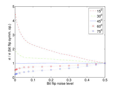
Figure 6: (color online) Variation of the ratio of standard deviation without any symmetry operation to the bit flip symmetry operation with increasing bit flip noise level.

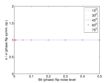
Figure 7: (color online) Variation of the ratio of standard deviation without any symmetry operation to the phase flip symmetry operation with increasing bit flip (phase flip) noise level.

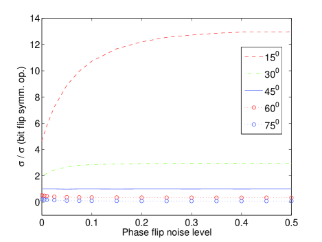
Figure 8: (color online) Variation of the ratio of standard deviation without any symmetry operation to the bit symmetry operation with increasing phase flip noise level.

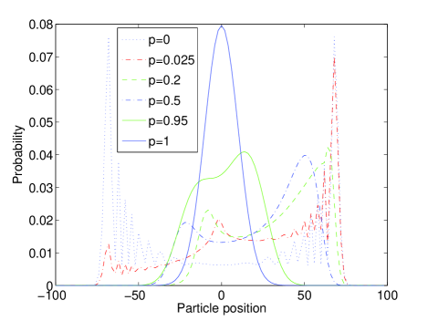
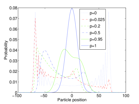
Figure 9: (color online) Amplitude damping channel acting on a Hadamard walker at temperature $T=0$. The distribution corresponding to intermediate values of $p$ clearly show the breakdown of the ${\bf RX}$ symmetry. However, the extended symmetry, ${\bf PRX}$ (where ${\bf P}$ stands for parity operation (spatial inversion)) holds good. This is observed at all temperatures. (a) Probability distribution of finding the particle undergoing unbiased quantum walk on which amplitude damping channel is acting. This shows that even at $T=0$, for sufficiently high coupling, the distribution turns classical. (b) Amplitude damping with bit flip symmetry.

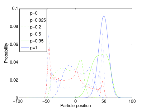
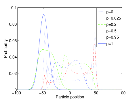
Figure 10: (color online) ${\bf PRX}$ symmetry seen to hold in biased quantum walk subjected to amplitude damping ($T=0$). The two cases are spatial inversions of each other. This holds for a generalized amplitude damping at any temperature. (a) walker with $\theta=30^{\circ}$ and bit flip; (b) $\theta=60^{\circ}$.

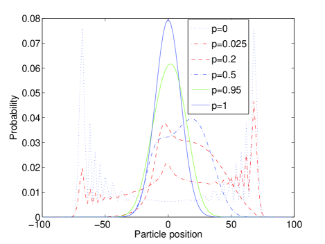
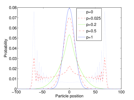
Figure 11: (color online) Onset of classicality is seen to be accentuated in a (Hadamard) quantum walk subjected to generalized amplitude damping with increasing temperatures. Figure (9(a)) depicts the $T=0$ case ($\chi=1$ in Eq. (75)). (a) Finite temperature corresponding to $\chi=0.75$ (b) $T=\infty$, corresponding to $\chi=0.5$. It may be noted that even at $T=\infty$, for sufficiently small coupling the distribution remains non-classical.

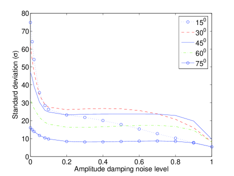
Figure 12: (color online) Variation of standard deviation with amplitude damping noise level for various value of $\theta$, $15^{\circ}$, $30^{\circ}$, $45^{\circ}$, $60^{\circ}$ and $75^{\circ}$. Note that the standard deviation for complementary angles converge to the same value.

Representing the walker distribution by its standard deviation $\sigma$, we may describe symmetry by the ratio of $\sigma$ without the symmetry operation to $\sigma$ with the symmetry operation. Figure 6 depicts the symmetry operation ${\bf X}$ for various bit flip noise levels. The convergence of the curves representing various $\theta$’s is a consequence of the complete randomization of the measured bit outcome in the computational basis. This implies that although X is not a symmetry of biased walk, it does become one in the fully classical limit. On the other hand, the symmetries ${\bf PRX}$ remain unaffected by noise. We note that, since the quantum walk here is evolved from the symmetric state $|0\rangle+i|1\rangle$, and the bit flip and phase flip noise are not partial to the state $|0\rangle$ or $|1\rangle$, this is equivalent to setting ${\bf P}$ to $1$, which explains the fact that the distributions in Figures 3 and 4 are spatially symmetric. Thus, ${\bf RX}$ by itself becomes a symmetry operation, which is manifested in the fact that in Figure 6 the values of the curve for complementary angles are the inverse of each other. Figure 7 shows that for either of the two noises, ${\bf Z}$ is a walk symmetry.

Figure 8 depicts the symmetry of the ${\bf RX}$ operation at all phase flip noise levels, as evident from that fact that the values of the curve for complementary angles are the inverse of each other. From Figures 6, 7 and 8, we note that for the Hadamard walk, all three symmetry operations ${\bf Z},{\bf X}$ and ${\bf R}$ are individually preserved. This is expected because here ${\bf P}=1$ as stated earlier, ${\bf R}=1$ by definition, so that the symmetry of ${\bf PRX}$ implies ${\bf X}=1$.

With the inclusion of bias and an initial arbitrary state, the full symmetries ${\bf Z}$ and ${\bf PRX}$ would be required, as proved by the following theorem.

Theorem 4

The operations ${\bf PRX}$ and ${\bf Z}$ are symmetries for the phase-flip and bit-flip channels.

Proof. We may look upon the phase flip channel (57) as a probabilistic mixture (in the discretized walk model) of $2^{n}$ quantum trajectories with $\Pi\in\{\mathbb{I},Z\}$. By virtue of Theorem 3, it suffices to show that any given unravelling is invariant under ${\bf Z}$ and ${\bf PRX}$. Consider an unravelling $\widehat{X}^{1}\equiv\cdots(IUB)(ZUB)(IUB)\cdots=\cdots(UB)(ZUB)(UB)\cdots$. This is the same as: $\cdots(UB)(UB^{\prime})(UB)\cdots$, where $B^{\prime}=ZB$, noting that $Z$ commutes with $U$. Now, ${\bf Z}\widehat{X}^{1}=\cdots(IZUB)(ZZUB)(IZUB)\cdots=\cdots(ZUB)(ZUB^{\prime})(ZUB)\cdots$, which, by Theorem 2, is equivalent to $\widehat{X}^{1}$. Now, ${\bf PRX}\widehat{X}^{1}=\cdots(PRX~{}UB)(Z~{}PRX~{}UB)(PRX~{}UB)\cdots=\cdots(PRX~{}UB)(PR~{}ZX~{}UB)(PRX~{}UB)\cdots=\cdots(PRX~{}UB)(PR~{}ZXZ~{}ZUB)(PRX~{}UB)\cdots=\cdots(PRX~{}UB)(PR~{}(-X)~{}UB^{\prime})(PRX~{}UB)\cdots$, which, by Theorem 2, is equivalent to $\widehat{X}^{1}$, since an overall phase factor of $\pm 1$ is irrelevant. Thus, the phase-flip channel is symmetric w.r.t. the operations ${\bf Z}$ and ${\bf PRX}$.

Regarding the bit-flip channel (62): as in the above case, consider an unravelling $\widehat{X}^{2}\equiv\cdots(UB)(XUB)(UB)\cdots$. This is the same as: $\cdots(UB)(U^{{\dagger}}B^{\prime\prime})(UB)\cdots$, where, as may be seen by direct calculation, $B^{\prime\prime}=XB$. Now, ${\bf Z}\widehat{X}^{2}=\cdots(Z~{}UB)(X~{}Z~{}UB)(Z~{}UB)\cdots=\cdots(Z~{}UB)(X~{}ZX~{}XUB)(Z~{}UB)\cdots=\cdots(Z~{}UB)((-Z)~{}U^{{\dagger}}B^{\prime\prime})(Z~{}UB)\cdots$, which, by Theorem 2, is equivalent to $\widehat{X}^{2}$, since an overall phase factor of $\pm 1$ is irrelevant.

Further, ${\bf PRX}\widehat{X}^{2}=\cdots(PRX~{}UB)(X~{}PRX~{}UB)(PRX~{}UB)\cdots=\cdots(PRX~{}UB)(PRX~{}X~{}UB)(PRX~{}UB)\cdots=\cdots(PRX~{}UB)(PRX~{}U^{{\dagger}}B^{\prime\prime})(PRX~{}UB)\cdots$, which, by Theorem 2, is equivalent to $\widehat{X}^{2}$. $\blacksquare$

IV.2 Decoherence via generalized amplitude damping channel

Here we study the behaviour of quantum walk subjected to a generalized amplitude damping (with temperature $T\geq 0$), which would reduce at $T=0$ to the amplitude damping channel. As an example of a physical process that realizes the generalized amplitude damping channel, we consider a two-level system interacting with a reservoir of harmonic oscillators, with the system-reservoir interaction being dissipative and of the weak Born-Markov type bp02 ; srienv06 leading to a standard Lindblad equation, which in the interaction picture has the following form srib06

$$\frac{d}{dt}\rho^{s}(t)=\sum_{j=1}^{2}\left(2R_{j}\rho^{s}R^{{\dagger}}_{j}-R_{j}^{{\dagger}}R_{j}\rho^{s}-\rho^{s}R_{j}^{{\dagger}}R_{j}\right),$$ (63)

where $R_{1}=(\gamma_{0}(N_{\rm th}+1)/2)^{1/2}R$, $R_{2}=(\gamma_{0}N_{\rm th}/2)^{1/2}R^{{\dagger}}$ and $N_{\rm th}=(\exp(\hbar\omega/k_{B}T)-1)^{-1}$, is the Planck distribution giving the number of thermal photons at the frequency $\omega$, and $\gamma_{0}$ is the system-environment coupling constant. Here $R=\sigma_{-}\cosh(r)+e^{i\Phi}\sigma_{+}\sinh(r)$, and the quantities $r$ and $\Phi$ are the environmental squeezing parameters and $\sigma_{\pm}=\frac{1}{2}\left(\sigma_{1}\pm i\sigma_{2}\right)$. For the generalized amplitude damping channel, we set $r=\Phi=0$. If $T=0$, so that $N_{\rm th}=0$, then $R_{2}$ vanishes, and a single Lindblad operator suffices.

The generalized amplitude damping channel is characterized by the following Kraus operators srib06 :

$$\begin{array}[]{ll}E_{0}\equiv\sqrt{\chi}\left[\begin{array}[]{ll}1&0\\ 0&\sqrt{1-p(t)}\end{array}\right];{}{}{}{}&E_{1}\equiv\sqrt{\chi}\left[\begin{array}[]{ll}0&\sqrt{p(t)}\\ 0&0\end{array}\right],\\ E_{2}\equiv\sqrt{1-\chi}\left[\begin{array}[]{ll}\sqrt{1-p(t)}&0\\ 0&1\end{array}\right];{}{}{}{}&E_{3}\equiv\sqrt{1-\chi}\left[\begin{array}[]{ll}0&0\\ \sqrt{p(t)}&0\end{array}\right],\end{array}$$ (74)

where

$$p(t)\equiv 1-e^{-\gamma_{0}(2N_{\rm th}+1)t};\hskip 28.45274pt\chi\equiv\frac{1}{2}\left[1+\frac{1}{2N_{\rm th}+1}\right].$$ (75)

When $T=0$, $\chi=1$, and for $T\rightarrow\infty$, $\chi=1/2$.

The density operator at a future time can be obtained as srib06

$$\rho^{s}(t)=\begin{pmatrix}{\frac{1}{2}}(1+A_{1})&A_{2}\cr A_{2}^{*}&{\frac{1}{2}}(1-A_{1})\end{pmatrix},$$ (76)

where

$$A_{1}\equiv\langle\sigma_{3}(t)\rangle=e^{-\gamma_{0}(2N_{\rm th}+1)t}\langle\sigma_{3}(0)\rangle-{\frac{1}{(2N_{\rm th}+1)}}\left(1-e^{-\gamma_{0}(2N_{\rm th}+1)t}\right),$$ (77)

$$A_{2}=e^{-{\frac{\gamma_{0}}{2}}(2N_{\rm th}+1)t}\langle\sigma_{-}(0)\rangle\rangle.$$ (78)

Figures 9, 10 and 11 depict the onset of classicality with increasing coupling strength (related to $p$) and temperature (coming from $\chi$). Figure 9, which shows the effect of an amplitude damping channel on a Hadamard walker at zero temperature, illustrates the breakdown of ${\bf RX}$ symmetry even though the initial state is $|0\rangle+i|1\rangle$. This is because, in contrast to the phase-flip and bit-flip channels, the generalized amplitude damping is not symmetric towards the states $|0\rangle$ and $|1\rangle$. However, the extended symmetry ${\bf PRX}$ is preserved both for Hadamard as well as biased walks, as seen from Figures 9 and 10, respectively.

From Figures (9(a)), (11(a,b)), the onset of classicality with increasing temperature is clearly seen. Figure 12 presents the standard deviation for quantum walks on a line with various biases, subjected to amplitude damping noise. The standard deviation for complementary angles ($\theta\leftrightarrow\pi/2-\theta$) is seen to converge to the same value in the fully classical limit. This may be understood as follows. First, we note that since ${\bf PRX}$ is a symmetry of the quantum walk, and the effect of ${\bf P}$ does not show up in the standard deviation plots, ${\bf RX}$ by itself is an apparent symmetry. Further, in the classical limit the measurement outcome being a unique asymptotic state for the (generalized) amplitude damping channel, effectively ${\bf X}\simeq 1$, which makes ${\bf R}$ a symmetry operation.

The following theorem generalizes Theorem 2 to an open system subjected to a generalized amplitude damping channel.

Theorem 5

The operations ${\bf Z}$ and ${\bf PRX}$ are symmetries for the generalized amplitude damping channel.

Proof. By virtue of Theorem 3, it suffices to show that any given unravelling is invariant under ${\bf Z}$ and ${\bf PRX}$. Consider an unravelling

$$\widehat{X}^{3} \equiv \cdots(E_{0}UB)(E_{1}UB)(E_{2}UB)(E_{3}UB)\cdots$$ (79a)

$$\equiv \cdots(UB_{(0)})(U^{{\dagger}}B_{(1)})(UB_{(2)})(U^{{\dagger}}B_{(3)})\cdots,$$ (79b)

where the non-unitary matrices are given by $B_{(j)}=E_{j}B$. Now,

$${\bf Z}\widehat{X}^{3} = \cdots(E_{0}ZUB)(E_{1}ZUB)(E_{2}ZUB)(E_{3}ZUB)\cdots$$ (80)

$$= \cdots(ZE_{0}UB)((-Z)E_{1}UB)(ZE_{2}UB)((-Z)E_{3}UB)\cdots$$

$$= \cdots(ZUB_{(0)})((-Z)U^{{\dagger}}B_{(1)})(ZUB_{(2)})((-Z)U^{{\dagger}}B_{(3)})\cdots$$

$$= \cdots(UB_{(0)}^{(1)})(-U^{{\dagger}}B_{(1)}^{(1)})(UB_{(2)}^{(1)})(-U^{{\dagger}}B_{(3)}^{(1)})\cdots$$

Ignoring the overall $\pm 1$ factor in Eq. (80), and comparing it with Eq. (79a), and noting that that the derivation of the proof of Theorem 2 did not require the matrices $B_{j}$ to be unitary, we find along similar lines that ${\bf Z}\widehat{X}^{3}$ is equivalent to $\widehat{X}^{3}$.

The following may be directly verified

$${\bf PRX}\widehat{X}^{3} = \cdots(E_{0}PRXUB)(E_{1}PRXUB)(E_{2}PRXUB)(E_{3}PRXUB)\cdots$$ (81a)

$$= \cdots(E_{0}UB^{(2)})(E_{1}UB^{(2)})(E_{2}UB^{(2)})(E_{3}UB^{(2)})\cdots$$ (81b)

$$= \cdots(UB_{(0)}^{(2)})(U^{{\dagger}}B_{(1)}^{(2)})(UB_{(2)}^{(2)})(U^{{\dagger}}B_{(3)}^{(2)})\cdots,$$ (81c)

which, by Theorem 2, is equivalent to $\widehat{X}^{3}$. For proof of Eq. (81b), see the proof of Theorem 1. Eq. (81c) is obtained analogously to Eq. (79b), except that the matrix $B^{(2)}$ is used instead of $B$. $\blacksquare$

This may be expressed by the statement

$${\cal N}\widehat{W} \simeq {\cal N}{\bf Z}\widehat{W},$$ (82a)

$${\cal N}\widehat{W} \simeq {\cal N}{\bf PRX}\widehat{W},$$ (82b)

which generalizes Eq. (19). These results show that the symmetries persist for dephasing (phase flip), bit flip and (generalized) amplitude damping channels.

V Quantum walk on a cycle

In this work, though we are primarily concerned with symmetries for a quantum walk on a line, and the influence of noise on them, we briefly consider in this Section an extension of the above ideas to quantum walks on a cycle. Further extensions would be quantum walks on a more general graph vk06 ; om06 or in higher dimensions $d>2$ mac02 . In the former, the 1D walk is generalized to $N$-cycles and to hypercubes, including the effect of phase noise in the coin space, and decoherence in position space. In the latter, the Hadamard transformation is generalized to a non-entangling tensor product of Hadamards, or to an entangling discrete Fourier transform or the Grover operator. They bring in many novel features absent in the quantum walk on a line. Here we will restrict ourselves to pointing out that quantum walk on a cycle differs considerably from walk on a line, both with respect to symmetry operations as well as noise.

In contrast to the case of quantum walk on a line, none of the four discrete symmetries of Theorem 1 hold in general for unitary quantum walk on a cycle or closed path. Thus, if $B$ in Eq. (6) is replaced by any of $B^{(1)}$, $B^{(2)}$, $B^{(3)}$, or $B^{(4)}$, given by Eq. (17), the spatial probability distribution is not guaranteed to be the same.

Theorem 6

The operation $G:B\rightarrow B^{\star}$ is in general not a symmetry of the quantum walk on a cycle.

Proof. For the cyclic case, in place of Eq. (III), we now have

$$|\Psi_{1}\rangle = (UB)^{n}|\alpha,\beta\rangle=\sum_{j_{1},j_{2},\cdots,j_{n}}b_{j_{n},j_{n-1}}\cdots b_{j_{2},j_{1}}b_{j_{1},\alpha}|j_{n},\beta+2J-n~{}({\rm mod}~{}R)\rangle,$$ (83a)

$$|\Psi_{2}\rangle = (UB^{(1)})^{n}|\alpha,\beta\rangle=\sum_{j_{1},j_{2},\cdots,j_{n}}b_{j_{n},j_{n-1}}\cdots b_{j_{2},j_{1}}b_{j_{1},\alpha}(e^{i\phi})^{j_{n-1}+\cdots+j_{1}+\alpha}|j_{n},\beta+2J-n~{}({\rm mod}~{}R)\rangle,$$ (83b)

where $R$ is the number of sites in the cycle. For an arbitrary state $|a,b\rangle$ in the computational-and-position basis, we have

$$\langle a,b|\Psi_{1}\rangle = \sum_{j_{1},j_{2},\cdots,j_{n-1}\in{\cal J}}b_{a,j_{n-1}}\cdots b_{j_{2},j_{1}}b_{j_{1},\alpha}$$ (84a)

$$\langle a,b|\Psi_{2}\rangle = \sum_{j_{1},j_{2},\cdots,j_{n-1}\in{\cal J}}b_{a,j_{n-1}}\cdots b_{j_{2},j_{1}}b_{j_{1},\alpha}(e^{i\phi})^{j_{n-1}+\cdots+j_{1}+\alpha}$$ (84b)

$$\equiv \sum_{j_{1},j_{2},\cdots,j_{n-1}\in{\cal J}}b_{a,j_{n-1}}\cdots b_{j_{2},j_{1}}b_{j_{1},\alpha}(e^{i\phi\epsilon}),$$

where ${\cal J}$ is the set of binary $(n-1)$-tuples $j_{1},j_{2},\cdots,j_{n-1}$ such that $J=j_{1}+j_{2}+\cdots+j_{n-1}+a$ satisfies $b=\beta+2J-n~{}({\rm mod}~{}R)$. We find that $\epsilon=\alpha-a+J$ and $J=(b+n-\beta)/2+mR$, where $m=0,1,2,\cdots,\lfloor n/R\rfloor$. Thus, the terms in the superposition (84a) are not in general identical with those in (84b), apart from a common factor, unless $\phi=0,2\pi,4\pi,\cdots$. A similar argument can be used to show that the terms in $\langle\overline{a},b|\Psi_{1}\rangle$ are not in general the same as those in $\langle\overline{a},b|\Psi_{2}\rangle$. Given the independence of $\phi$ from the coefficients $b_{j_{2},j_{1}}b_{j_{1},\alpha}$, it is not necessary that $|\langle a,b|\Psi_{1}\rangle|^{2}+|\langle\overline{a},b|\Psi_{1}\rangle|^{2}=|\langle a,b|\Psi_{2}\rangle|^{2}+|\langle\overline{a},b|\Psi_{2}\rangle|^{2}$. The equality holds in general (for arbitrary unitary matrix $B$ and time parameter $n$) if and only if $\phi=0,2\pi,4\pi,\cdots$. Repeating the argument for $B^{(2)}$, $B^{(3)}$ and $B^{(4)}$, we find that all the four discrete symmetries of Theorem 1 break down in general. $\blacksquare$

We note that for phase flip symmetry, where $e^{i\phi}=-1$, the superposition terms in Eq. (84b) may differ from the corresponding terms in Eq. (84a) only with respect to sign. Given that all the terms like $b_{j_{2},j_{1}}$, $b_{j_{1},\alpha}$, etc. are built from a small set of trignometric functions of the three parameters $\theta$, $\zeta$ and $\xi$, certain values of $n$ may render the right hand sides of Eqs. (84a) and (84b) equal. However in general, this equality will not hold for arbitrary $n$.

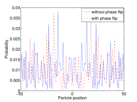
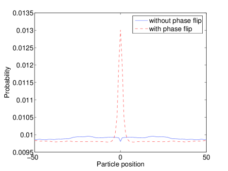
Figure 13: (color online) An instance of breakdown of phase flip symmetry in a unitary quantum walk on a cycle, where the two extreme points (located at positions $\pm 50$) on the plot are spatially adjacent. The number of sites is 101 and $t=5000$ (in units of discrete time-steps), with bias angle $\theta=30^{\circ}$. (a) The solid curve represents the positional probability distribution without any symmetry operation applied, while the dashed curve represents that with a phase flip operation applied at each walk step. (b) The same as the above, but with time-averaging applied over every 50 steps, in order to more clearly bring out the breakdown in symmetry.

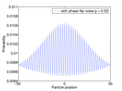
Figure 14: (color online) Restoration of phase flip symmetry in a noisy quantum walk on a cycle, where the two extreme points on the plot are spatially adjacent. The number of sites is 101 and $t=5000$ (in units of discrete time-steps), with bias angle $\theta=30^{\circ}$. The figure depicts the position probability distribution with or without phase flip symmetry operation applied at each step, with phase damping noise level $p=0.02$ [Eq. (57)]. After sufficiently long time, the quantum walk reaches the uniform distribution, typical of classical random walk.

An instance of breakdown of phase flip symmetry in the unitary quantum walk on a cycle is demonstrated in the example of Figure 13. The profile of the position probability distribution varies depending on the number of sites and the evolution time. Remarkably, this symmetry is restored above a threshold value of noise. The pattern in Figure 14 corresponds to phase noise with $p=0.02$ applied to a quantum walk, either with or without a phase flip symmetry operation. We note that the introduction of noise tends to classicalize the random walk, hence causing it to asymptotically reach a uniform distribution vk06 ; om06 . The above-mentioned symmetry restoration happens well before the uniformity sets in. The initial lack of symmetry gradually transitions to full symmetry as the noise level is increased. Thus, the role of symmetry operations and noise is quite different in the case of quantum walk on cycles as compared with that on a line.

A more detailed treatment of symmetries and noise in a quantum walk on a cycle and general graphs of other topologies will be presented elsewhere new .

VI Experimental realization in physical systems

Experimental realization of quantum walk using any of the proposed schemes is not free from noise due to environmental conditions and instrumental interference. In particular, noise can be a major issue in the scaling up of the number of steps in already realized quantum walk systems. Understanding the symmetries of the noisy and noiseless quantum walk could greatly help in the improvement of known techniques and in further exploration of other possible systems where quantum walk can be realized on a large scale. In this section we discuss the realization in a nuclear magnetic resonance (NMR) quantum-information processor and ultra-cold atomic systems.

VI.1 NMR quantum-information processor

Continuous time du and discrete time ryan quantum walk have been successfully implemented in a nuclear magnetic resonance (NMR) quantum-information processor. Considering the benefits of the effect of decoherence on the quantum walk viv ; brun , Ref. ryan has also experimentally added decoherence on the discrete time quantum walk by implementing dephasing in NMR. By adding decoherence after each step they have shown the transition of quantum walk to the classical random walk.

In NMR spectroscopy of the given system (molecule) the extent of its isolation from the environment is determined in terms of its phase coherence time $T_{2}$ and its energy relaxation time $T_{1}$. If the pulse sequence is applied to the NMR quantum-information processor within the time $T<{T_{2},T_{1}}$, the system is free from the environmental effects. The pulse sequence exceeding the time $T_{2}$ can be considered to affected by the dephasing channel and the pulse sequence exceeding the time $T_{1}$ can be considered to be affected by the amplitude damping channel. In experiments of time scale greater than the time $T_{2}$ or $T_{1}$, a refocusing pulse sequence is applied to compensate for the environmental effects. In Ref. ryan the pulse sequence for the quantum walk was implemented within the time $T_{1}$ and $T_{2}$.

The environmental effect (noise) on quantum walk symmetries presented in this article can be verified in the NMR system by scaling up the number of steps of quantum walk realized. By applying a controlled amount of the refocusing pulse sequence, the effect of different levels of noise can be experimentally verified.

VI.2 Ultra-cold atoms

There have been various schemes suggested to implement quantum walks using neutral atoms in an optical lattice rauss ; eckert . In Ref. mandel , the controlled coherent transport and splitting of atomic wave packets in spin dependent optical lattice has been experimentally demonstrated using rubidium atoms. A Bose-Einstein condensate of up to $3\times 10^{5}$ atoms is initially created in a harmonic magnetic trap. A three dimensional optical lattice is superimposed on the Bose-Einstein condensate and the intensity is raised in order to drive the system into a Mott insulating phase greiner .

Two of the three orthogonal standing wave light fields is operated at one wavelenght, $\lambda_{y,z}=840$ nm and the third along the horizontal direction is tuned to the wavelength $\lambda_{x}=785$ nm between the fine structure splitting of the rubidium $D1$ and $D2$ transitions. Along this axis a quarter wave plate and an electro-optical modulator (EOM) is placed to allow the dynamic rotation of the polarization vector of the retro-reflected laser beam through an angle $\theta$ by applying an appropriate voltage to the EOM. After reaching the Mott insulating phase, the harmonic magnetic field is completely turned off but a homogeneous magnetic field along the $x$ direction is maintained to preserve the spin polarization of the atoms. The light field in the $y$ and $z$ direction is adiabatically turned off to reduce the interaction energy, which strongly depends on the confinement of the atoms at a single lattice site.

A standing wave configuration in the $x$ direction is used to transport the atoms. By changing the linear polarization vector enclosing angle $\theta$, the separation between the two potentials is controlled. By rotating the polarization angle $\theta$ by $\pi$, with the atom in a superposition of internal states, the spatial wave packets of the atom in the $|0\rangle$ and the $|1\rangle$ state are transported in opposite directions. The final state after such a movement is then given by $1/\sqrt{2}(|0,x-1\rangle+i\exp(i\beta_{p})|1,x+1\rangle)$. The phase $\beta_{p}$ between the separated wave-packets depends on the accumulated kinetic and potential energy phases in the transport process and in general will be nonzero. The coherence between the two wave-packets is revealed by absorption imaging of the momentum distribution. A $\pi/2$ microwave pulse is applied before absorption imaging to erase the which-way information encoded in the hyperfine states.

However, to increase the separation between the two wave-packets further, one could increase the polarization angle $\theta$ to integer multiples of $180^{\circ}$. To overcome the limitation of the maximum voltage that can be applied to the EOM, a $\pi$ pulse after the polarization is applied, thereby swapping the roles of the two hyperfine states. The single particle phase $\beta_{p}$ remains constant throughout the atomic cloud and is reproducible. After the absorption imaging a Gaussian envelope of the interference pattern is obtained.

One can build up on the above technique to implement a quantum walk which introduces phase along with each splitting (step). The above setup can be modified by dividing the separations into small steps and introducing a $\pi/2$ pulse after each separation without intermediate imaging. A phase $\beta_{p}$ is introduced in each step. The absorption imaging of the distribution of the atomic cloud after $n$ steps would give the interference pattern of the quantum walk.

This effect of the addition of phase during the quantum walk process can be easily understood from the phase damping channel and arbitrary phase rotation presented in this article. The addition of $\pi$ pulse to overcome the limit of EOM is a bit flip operation in the quantum walk.

There have been other proposals for physical realization of quantum walk using Bose-Einstein condensate (BEC) chandra06 where the unitary shift operator induces a bit flip. A stimulated Raman kick is used as a unitary shift operator to translate the Bose-Einstein condensate in the Schrödinger cat state to a superposition in position space. Two selected levels of the atoms in the Bose-Einstein condensate are coupled to the two modes of counter-propagating laser beams. The stimulated Raman kick, in imparting a translation in position space, also flips the internal state of the Bose-Einstein condensate. An rf pulse ($\pi$ pulse) is suggested as a compensatory mechanism to flip the internal state of the condensate back to its initial value after every unitary shift operator. From the ${\bf PRX}$ symmetry pointed in this article, it follows that there is no need for the compensatory operation for an unbiased quantum walk started in the state $|0\rangle+i|1\rangle$. The availability of walk symmetries could also be useful for exploring other possible physical implementations which induce such symmetry operations along with the translation.

In the most widely studied version of quantum walk, a quantum coin toss (Hadamard operation) is used after every displacement operation. Continuous external operations on a particle confined in a trap reduces the confinement time of the particle. Reducing the number of external operations will benefit the scaling up of the number of steps of the quantum walk. One can workout a system where the quantum coin toss operation is eliminated by transferring the burden of evolving the particle in superposition of the internal state to the displacement operator itself chandra062 ; css . Such a transfer may introduce additional operations that correspond to the walk symmetry, and may thus be ignored. Further, systems of this kind are expected to be affected by amplitude damping as one of the states might be more stable than the other one in the trap. The present work could help to optimize such a noisy quantum walk.

In a scheme suggested using quantum accelerator mode ma , different internal states of an atom receive different momentum transfer with each alternative kick, giving different walking speeds in the two directions and this can be seen as a biased walk. Our study of symmetry in a noisy, biased quantum walk could help improve the above technique and make it easier for its experimental realization.

VII Conclusions

Our work considers variants of quantum walks on a line which are equivalent in the sense that the final positional probability distribution remains the same in each variant. In particular, we consider variants obtained by the experimentally relevant operations of $Z$ or $X$ applied at each quantum walk step, with the symmetry operations given by ${\bf Z}$ and ${\bf PRX}$. This could be experimentally advantageous since practical constraints may mean that one of the variants is preferred over the rest. A specific example is the simplification of the implementation of quantum walk using a Bose-Einstein condensate with a stimulated Raman kick providing the conditional translation operation. What is especially interesting is that these symmetries are preserved even in the presence of noise, in particular, those characterized by the phase flip, bit flip and generalized amplitude damping channels. This is important because it means that the equivalence of these variants is not affected by the presence of noise, which would be inevitable in actual experiments. The symmetry of the phase operation under phase noise is intuitive, considering that this noise has a Kraus representation consisting of operations that are symmetries of the noiseless quantum walk. However, for the PRX symmetry under phase noise, and for any symmetry under other noisy channels (especially in the case of generalized amplitude damping channel), the connection was not obvious before the analysis was completed.

Our results are supported by several numerical examples obtained by evolving the density operator in the Kraus representation. However, analytical proofs of the effect of noise on symmetries are obtained using the quantum trajectories approach, which we find convenient for this situation. We also present the quantum walk on the cycle, which can be generalized to any closed graph. An interesting fact that comes out is that the symmetry breaks down in general but is restored above a certain noise level. Some representative plots demonstrating the effect of the phase damping channel on phase flip symmetry are presented.

Finally we have discussed the experimental realization of quantum walk in a physical system, such as NMR and ultra cold atoms, as examples where these studies can be beneficial for improving the efficiency of the implementation on large scales.

References

- (1) M. N. Barber and B. W. Ninham, Random and Restricted walks: Theory and Applications (Gordon and Breach, New York, 1970).
- (2) S. Chandrasekhar, Rev. Mod. Phys. 15, 1 (1943).
- (3) M. Jerrum and A. Sinclair, The Markov chain Monte Carlo method: An approach to approximate counting and integration, Edited by Dorit S. Hochbaum, in (Approximation Algorithm for NP-hard Problems, PWS Publishing, Boston), chapter 12, p.482-520. (1996).
- (4) Y. Aharonov, L. Davidovich and N. Zagury, Phys. Rev. A 48, 1687, (1993).
- (5) J. Kempe, Contemp. Phys. 44, 307 (2003).
- (6) A. M. Childs, R. Cleve, E. Deotto, E. Farhi et al., in Proceedings of the 35th ACM Symposium on Theory of Computing (ACM Press, New York, 2003), p.59.
- (7) N. Shenvi, J. Kempe and K. Birgitta Whaley, Phys. Rev. A 67, 052307, (2003).
- (8) A. M. Childs, J. Goldstone, Phys. Rev. A 70, 022314, (2004).
- (9) A. Ambainis, J. Kempe and A. Rivosh, e-print quant-phy/0402107.
- (10) C. A. Ryan, M. Laforest, J. C. Boileau, and R. Laflamme, Phys. Rev. A 72, 062317, (2005).
- (11) J. Du, H. Li, X. Xu, M. Shi et al., Phys. Rev. A 67, 042316, (2003).
- (12) B. C. Travaglione and G. J. Milburn, Phys. Rev. A 65, 032310, (2002).
- (13) W. Dur, R. Raussendorf, V. M. Kendon and H.J. Briegel, Phys. Rev. A 66, 052319, (2002).
- (14) K. Eckert, J. Mompart, G. Birkl and M. Lewenstein, Phys. Rev. A 72, 012327, (2005).
- (15) C. M. Chandrashekar, Phys. Rev. A 74, 032307 (2006).
- (16) Z.-Y. Ma, K. Burnett, M. B. d’Arcy, and S. A. Gardiner, Phys. Rev. A 73, 013401, (2006).
- (17) V. M. Kendon and B. C. Sanders, Phys. Rev. A 71, 022307 (2005).
- (18) T. A. Brun, Am. J. of Phys. 70, 719 (2002).
- (19) M. Nielsen and I. Chuang, Quantum Information and Quantum Computation (Cambridge University Press, 2000).
- (20) S. Banerjee and R. Srikanth, eprint quant-ph/0611161.
- (21) H.-P. Breuer and F. Petruccione, The Theory of Open Quantum Systems (Oxford University Press, 2002).
- (22) R. Srikanth and S. Banerjee, to appear in Phys. Lett. A; eprint quant-ph/0611263.
- (23) V. Kendon, eprint quant-ph/0606016;
- (24) O. Maloyer and V. Kendon, eprint quant-ph/0612229.
- (25) T. D. Mackay, S. D. Bartlett, L. T. Stephenson and B. C. Sanders, J. Phys. A: Math. Gen 35, 2745 (2002).
- (26) S. Banerjee, R. Srikanth and C. M. Chandrashekhar, under preparation.
- (27) V. Kendon and B. Tregenna, Phys. Rev. A 67, 042315 (2003).
- (28) T.A. Brun, H.A. Carteret, and A. Ambainis, Phys. Rev. Lett. 91, 130602 (2003).
- (29) O. Mandel, M. Greiner, A. Widera, T. Rom et al., Phys. Rev. Lett. 91, 010407 (2003).
- (30) M. Greiner, O. Mandel, T. Esslinger, T.W. Hänsch, et al., Nature (London) 415, 39 (2002).
- (31) C. M. Chandrashekar, eprint quant-ph/0609113.
- (32) C. M. Chandrashekar, S. Banerjee and R. Srikanth, under preparation.