Quasi-exact solutions for two interacting electrons in two-dimensional anisotropic dots

Abstract

We present an analysis of the two-dimensional Schrödinger equation for two electrons interacting via Coulombic force and confined in an anisotropic harmonic potential. The separable case of $\omega_{y}:\omega_{x}=2$ is studied particularly carefully. The closed-form expressions for bound-state energies and the corresponding eigenfunctions are found at some particular values of $\omega_{x}$. For highly-accurate determination of energy levels at other values of $\omega_{x}$, we apply an efficient scheme based on the Fröbenius expansion.

1 Introduction

The Hookean system composed of $N$ interacting particles trapped in an external harmonic potential

$$V(\textbf{r})={m_{*}\over 2}[\omega_{x}^{2}{x}^{2}+\omega_{y}^{2}{y}^{2}+\omega_{z}^{2}{z}^{2}]$$ (1)

has been considered first as a model of nucleus in the early days of nuclear physics [1]. In the case the two particles interact via central forces, the Hookean system enjoys a particularly nice feature that the center-of-mass motion may be separated out. Because of its relatively easy tractability, the system has nowadays become a standard tool for testing quality of many-body approximation methods in studying correlations between electrons. Recently, the Hookean system attracted renowned interest, since the progress in semiconductor technology has allowed the formation of quantum dots (QDs), which are the systems of few electrons confined on the scale of hundreds of nanometers in an approximately harmonic potential [2]. For the simplest QD, consisting of two electrons ($N=2$), the Hamiltonian can be written as

$$H=\sum_{i=1}^{2}[{\textbf{p}_{i}^{2}\over 2m_{*}}+V(\textbf{r}_{i})]+{e^{2}\over\varepsilon_{*}|\textbf{r}_{2}-\textbf{r}_{1}|},~{}~{}~{}~{}$$ (2)

where $m_{*}$ is the effective electron mass and $\varepsilon_{*}$ the effective dielectric constant. Introducing center of mass and relative coordinates

$$\textbf{R}={1\over 2}(\textbf{r}_{1}+\textbf{r}_{2})=(X,Y,Z),~{}\textbf{r}=\textbf{r}_{2}-\textbf{r}_{1}=(x,y,z),$$ (3)

the above Hamiltonian is separated into $H=H^{\textbf{R}}+H^{\textbf{r}}$, where the center of mass Hamiltonian

$$H^{\textbf{R}}={\textbf{P}^{2}\over 4m_{*}}+m_{*}(\omega_{x}^{2}X^{2}+\omega_{y}^{2}Y^{2}+\omega_{z}^{2}Z^{2})$$ (4)

is exactly solvable. The problem is thus reduced to the Schrödinger equation for the relative motion

$$H^{\textbf{r}}\psi=\varepsilon^{\textbf{r}}\psi,$$ (5)

described by the Hamiltonian

$$H^{\textbf{r}}=-\hbar^{2}\nabla^{2}/m_{*}+{m_{*}\over{4}}[{\omega}_{x}^{2}x^{2}+{\omega}_{y}^{2}y^{2}+{\omega}_{z}^{2}z^{2}]+{e^{2}\over\varepsilon_{*}r},$$ (6)

where $r=|\textbf{r}|$. By a transformation $\hat{x}={x/a_{*}},\hat{y}={y/a_{*}}$, the relative motion equation is rescaled to the form

$$[-{\partial^{2}\over\partial\hat{x}^{2}}-{\partial^{2}\over\partial\hat{y}^{2}}-{\partial^{2}\over\partial\hat{z}^{2}}+\hat{\omega}_{x}^{2}\hat{x}^{2}+\hat{\omega}_{y}^{2}\hat{y}^{2}+\hat{\omega}_{z}^{2}\hat{z}^{2}+{1\over{\sqrt{\hat{x}^{2}+\hat{y}^{2}+\hat{z}^{2}}}}]\psi=\hat{\varepsilon}^{\textbf{r}}\psi$$ (7)

where $\varepsilon^{\textbf{r}}=R^{*}\hat{\varepsilon}^{\textbf{r}}$, $\omega_{x,y,z}/2=\hat{\omega}_{x,y,z}(\hbar/m_{*}a_{*}^{2})$ with the effective Bohr radius $a_{*}=\hbar^{2}\varepsilon_{*}/m_{*}e^{2}$ and the effective Rydberg constant $R^{*}=m_{*}e^{4}/\hbar^{2}\varepsilon_{*}^{2}$. In the following, we skip the hats over spatial coordinates $x,y,z$, frequencies $\omega_{x,y,z}$ and relative energy $\varepsilon^{\textbf{r}}$.

In the case of some particular relation between the frequencies $\omega_{x}$, $\omega_{y}$ and $\omega_{z}$, the problem of the relative motion becomes easier to solve, and at some specific values of frequencies it even appears quasi-solvable, i.e. one of the states of the spectrum can be analytically determined. The most studied example, important for describing QDs in a constant magnetic field, is the case the two of confinement frequencies are equal, e.g. $\omega_{x}=\omega_{y}=\omega$. For such axially symmetric system there are three cases where the problem of the relative motion (7) is integrable: 1) $\omega_{z}=\omega$, being separable in spherical coordinates, 2) $\omega_{z}:\omega=2$, being separable in parabolic coordinates, and 3) $\omega_{z}:\omega=1/2$, which is one of few examples of integrable problems that is generally not separable [3]. The quasi-solvability of the case 1) has been known for longtime [4, 5], and recently it has been demonstrated [6] that also in two other cases, one of the bound-state solutions (not necessarily the ground-state) can be obtained in a closed-form at some particular values of $\omega$.

Another example, which is important in studying two-dimensional (2D) QDs, is that where one of the frequencies is much larger than the other two, e.g. $\omega_{z}\rightarrow\infty$. The 2D approximation is usually justified in practice, since QDs are realized by lateral confinement of electron gas at the boundaries of semiconductor nanostructures. The above problem is integrable in two cases: that of $\omega_{x}=\omega_{y}$, and that of $\omega_{y}:\omega_{x}=2$ (which is equivalent to the case of $\omega_{y}:\omega_{x}=1/2$, under the exchange of $\omega_{x}$ and $\omega_{y}$). In the first case, the harmonic potential has circular symmetry and the problem of the relative motion becomes separable in polar coordinates. This case was much studied in the literature [7, 8, 9] and the closed-form solutions for particular frequencies have been derived [10]. The influence of the anisotropy aspect ratio $\omega_{x}/\omega_{y}$ on the QDs properties has been recently studied in Ref. [11, 12], where the separability of the case of $\omega_{y}:\omega_{x}=2$ in parabolic coordinates has been pointed out. Here we shall study this integrable case in detail. The main result of our paper is the demonstration that for particular values of $\omega_{x}$ the exact solutions can be found in a closed form. Although the property of quasi-solvability appears only at particular confinement frequencies, it is very appealing, as the knowledge of exact bound-state energies and the corresponding eigenfunctions in a closed form can be used for extracting information about the model and for testing the performance of approximation methods. Therefore, we discuss the quasi-solvable cases in detail, providing the values of confinement frequencies $\omega_{x}$ as well as the corresponding energy eigenvalues and the closed-form solutions for wave-functions. For determining the energy spectrum at arbitrary values of $\omega_{x}$, we develop a numerical scheme based on the Fröbenius method (FM), which was successfully used for calculating bound state energies of one-dimensional [13, 14, 15] and spherically symmetric potentials [16, 17]. The comparison of the bound-state solutions determined within the FM with the exact ones allows us to demonstrate how good is the performance of the numerical approximation scheme.

The outline of our work is as follows. In section 2, we give a brief discussion of the spectrum in 2D case of motion (8), paying a particular attention to the integrable case of $\omega_{y}:\omega_{x}=2$. In section 3, the quasi-solvable cases are derived. In section 4, the calculation within the FM are described and a comparison with exact results is given. The paper ends with concluding remarks in section 5.

2 Theoretical study

In the case of laterally confined QD, the relative motion equation (7) takes the form

$$[-{\partial^{2}\over\partial{x}^{2}}-{\partial^{2}\over\partial{y}^{2}}+{\omega}_{x}^{2}{x}^{2}+{\omega}_{y}^{2}{y}^{2}+{1\over{\rho}}]\psi(\mathbf{r})={\varepsilon}^{\textbf{r}}\psi(\mathbf{r}),$$ (8)

where $\rho=\sqrt{x^{2}+y^{2}}.$ The singlet (s) and triplet (t) spin states of the two-electron system correspond to symmetric and antisymmetric spatial wave-functions, respectively. As the centre-of-mass coordinate remains the same upon the interchange of electrons, the symmetry requirement reduces to the symmetry of the relative wave-function under inversion $\mathbf{r}\rightarrow-\mathbf{r}$ . Because of the invariance of equation (8) to reflections about the $x$- and $y$-axis, the $(x,y)$-parity of spatial wave-functions is well-defined. The parity $(+,+)$ or($-,-)$ corresponds to spin singlet eigenfunctions, and the parity $(+,-)$ or $(-,+)$ to the spin triplet ones.

The simplest case of circular symmetry has been much studied in the literature [7, 8, 9]. Here we discuss the other integrable case, $\omega_{y}:\omega_{x}=2$. Introducing two-dimensional parabolic coordinates through

$$x=\eta_{1}\eta_{2},y={1\over 2}(\eta_{1}^{2}-\eta_{2}^{2}),\eta_{2}\geq 0$$ (9)

the Schrödinger equation is transformed into the form

$$H^{\textbf{r}}(\eta_{1},\eta_{2})\psi(\eta_{1},\eta_{2})=\varepsilon^{\textbf{r}}\psi(\eta_{1},\eta_{2})$$ (10)

with the Hamiltonian given by

$$H^{\textbf{r}}(\eta_{1},\eta_{2})={1\over\eta_{1}^{2}+\eta_{2}^{2}}[-{\partial^{2}\over\partial\eta_{1}^{2}}-{\partial^{2}\over\partial\eta_{2}^{2}}+{1\over 4}\omega_{y}^{2}(\eta_{1}^{6}+\eta_{2}^{6})$$

$$-{1\over 4}\eta_{1}^{2}\eta_{2}^{2}(\eta_{1}^{2}+\eta_{2}^{2})(\omega_{y}^{2}-4\omega_{x}^{2})+2]$$ (11)

Now, it is easy to see that by setting $\omega_{y}=2\omega_{x}$ and $\psi(\eta_{1},\eta_{2})=g_{1}(\eta_{1})g_{2}(\eta_{2})$ into (11) one gets two ordinary differential equations of the identical form

$$[-{d^{2}\over d\eta_{j}^{2}}-\varepsilon^{\textbf{r}}\eta_{j}^{2}+\omega_{x}^{2}\eta_{j}^{6}+\beta_{j}]g_{j}(\eta_{j})=0,j=1,2$$ (12)

that are coupled by the condition $\beta_{1}+\beta_{2}=2$ to be satisfied by the separation constants $\beta_{1}$ and $\beta_{2}$. The integrability is explained by the fact that in the case of $\omega_{y}:\omega_{x}=2$ an operator commuting with the Hamiltonian (11) exists in the form [11]

$$\Lambda=\{\hat{L}_{z},\hat{p}_{x}\}+2\omega_{x}^{2}yx^{2}-{y\over\rho},$$ (13)

where the bracket $\{\}$ denotes anticommutator. The operator $\Lambda$ commutes with the $x-$reflection but anticommutes with the $y-$reflection operator, and its eigenvalue is given by $\delta=(\beta_{1}-\beta_{2})/2$. Therefore, the eigenstates corresponding to $\delta\neq 0$, i.e. $\beta_{1}\neq\beta_{2}$, are doubly degenerate with respect to the sign of $\delta$, and those with $\delta=0$, i.e. $\beta_{1}=\beta_{2}$, are nondegenerate.

The bound-states of the QD correspond to the values of $\varepsilon^{\textbf{r}}$ and $\beta_{j}$ such that the functions $\psi(\eta_{1},\eta_{2})$ vanish, as $|\eta_{1}|,\eta_{2}\rightarrow\infty$. The eigenfunctions of (12) which vanish at infinity can be ordered by the quantum number $n_{j}$ that counts its nodal points on $-\infty<\eta_{j}<\infty$, and will be denoted by $g^{(n_{j})}(\eta_{j},\beta_{j})$. The reflection symmetry of of (12) divides $g^{(n_{j})}(\eta_{j},\beta_{j})$ into two parity types, depending on $n_{j}$ being even or odd. As the inverse coordinate transformation

$$\eta_{1}=\frac{x}{|x|}\sqrt{\rho+y}\mbox{~{}~{}~{}~{}and~{}~{}~{}~{}}\eta_{2}=\sqrt{\rho-y},$$

shows discontinuity of in the $\eta_{1}$ coordinate at positive $y$-axis, the condition emerges that the solution of (10) be a product of functions of the same parity in $\eta_{1}$ and $\eta_{2}$, since only such products have the appropriate continuity properties in the whole space. In the case of $\delta=0$, which corresponds to the functions $g(\eta_{j},\beta_{j})$ having the same number of nodal points, the singlet state (s) with $(x,y)-$parity $(+,+)$ is represented by the product of functions being even in $\eta_{1}$ and $\eta_{2}$, while the triplet state (t) with $(-,+)$ is represented by the product of odd functions. For $\delta\neq 0$ the solutions of (10) with well-defined $(x,y)$-parity are easily constructed as

$$\psi_{(\pm)}^{(n_{1},{n_{2})}}(\eta_{1},\eta_{2})=g^{(n_{1})}(\eta_{1},\beta_{1})g^{(n_{2})}(\eta_{2},\beta_{2})\pm g^{(n_{1})}(\eta_{2},\beta_{1})g^{(n_{2})}(\eta_{1},\beta_{2}),$$ (14)

where the sign $(+)$ corresponds to the singlet/triplet state with $(x,y)-$parity $(+,+)$/$(-,+)$, and the sign $(-)$ to the triplet/singlet state with $(+,-)$/$(-,-)$ in the case of $n_{1}$ and $n_{2}$ being even/odd.

In order to visualize the manifestation of degeneracies discussed above, we consider the behavior of bound-state energies for varying anisotropy $\omega_{x}/\omega_{y}$. The numerical calculation have been performed with the help of the linear Rayleigh-Ritz method using the basis of two-dimensional harmonic oscillator eigenstates (”exact diagonalization”). The energies of low-lying states of the relative motion, $\varepsilon^{\textbf{r}}$, are plotted in figure 1, for a fixed frequency $\omega_{x}=0.5$ in function of the parameter $\omega_{y}$. It can be observed how the states with spatial parity, $(+,-)$,$(-,+)$ become degenerate with those of $(+,+),(-,-)$, respectively, in the case discussed above, i.e. $\omega_{y}:\omega_{x}=2$, and in the case equivalent to it after exchange $x\rightleftarrows y$, i.e. $\omega_{x}:{\omega_{y}}=2$. The visible degeneracy of the spectrum at $\omega_{y}=\omega_{x}=0.5$ corresponds to a circular symmetry of the harmonic potential.

Figure 1: The behaviour of the relative motion energy levels of a QD at $\omega_{x}=0.5$ in function of $\omega_{y}$. The vertical lines correspond to the cases $\omega_{x}:\omega_{y}=2$ and $\omega_{y}:\omega_{x}=2$. The circularly symmetric case of $\omega_{y}=\omega_{x}$ is marked by the broken line.

In the following we will discuss the spectrum of the anisotropic QD in the case of $\omega_{y}:\omega_{x}=2$, which can be determined by solving a coupled pair of one-dimensional equations (12). A simple scheme based on the FM will be used for the numerical determination of the solutions in the above case. The exact solution will be provided for particular values of $\omega_{x}$.

3 Exact solutions

Let us to come to main purpose of this paper which is the demonstration that the problem of a 2D QD, confined by the potential ${\omega}_{x}^{2}{x}^{2}+{\omega}_{y}^{2}{y}^{2}$, is quasi-solvable for ${\omega}_{y}:{\omega}_{x}=2$, i.e. that some of the solutions of the relative motion equation (8) can be found algebraically for certain values of $\omega_{x}$. We are looking for a solution of the form $\psi(\eta_{1},\eta_{2})=g(\eta_{1},\beta_{1})g(\eta_{2},\beta_{2})$, where $\beta_{1}+\beta_{2}=2$, and $g(\eta_{j},\beta_{j})$ fulfils the ordinary differential equation (12). As the form of Eq.12 is similar to that of the sextic anharmonic oscillator, the quasi exact solutions can be represented as [18]

$$g(\eta_{j},\beta_{j})=e^{-{{\omega_{x}\eta_{j}^{4}\over 4}}}\sum_{i=0}^{\infty}a_{i}^{(j)}\eta_{j}^{2i+\nu},$$ (15)

where $a_{0}^{(j)}\neq 0$, and $\nu=0,1$ correspond to the even- and odd-parity case, respectively. Substituting (15) into (12) and comparing the coefficients of like powers of $\eta_{j}$, one gets the three-term recursion relation for the expansion coefficients $a_{i}^{(j)}$ in the form

$$A_{i}a_{i+1}^{(j)}+B_{i}^{(j)}a_{i}^{(j)}+C_{i}a_{i-1}^{(j)}=0,$$ (16)

where

$$A_{i} = (2i+\nu+1)(2i+\nu+2)$$

$$B_{i}^{(j)} = -\beta_{j}$$

$$C_{i} = \varepsilon^{\textbf{r}}+(1-4i-2\nu)\omega_{x}$$ (17)

with $a_{i}^{(j)}=0$ for $i<0$. It turns out that the QD equation (8) is exactly solvable if the series in the representations (15) for both $g(\eta_{1},\beta_{1})$ and $g(\eta_{2},\beta_{2})$, terminate after a finite number of terms. This gives the three conditions

$$\varepsilon^{\textbf{r}}=\omega_{x}(3+4n+2\nu)$$ (18)

$$a_{n+1}^{(1)}(\omega_{x},\varepsilon^{\textbf{r}},\beta_{1})=0\mbox{~{}~{}~{}~{}and~{}~{}~{}~{}}a_{n+1}^{(2)}(\omega_{x},\varepsilon^{\textbf{r}},\beta_{2})=0,$$ (19)

where $n$ denotes the number of the highest non-vanishing term which appears to be necessarily the same in both series. Using the recurrence relation (16), the coefficients of the series may be conveniently represented in the form

$$a_{n+1}^{(j)}(\omega_{x},\varepsilon^{\textbf{r}},\beta_{j})={(-1)^{n+1}a_{0}^{(j)}\over(2(n+1)+\nu)!}P_{n}^{(j)}(\varepsilon^{\textbf{r}},\beta_{j},\omega_{x})=$$

$${(-1)^{n+1}a_{0}^{(j)}\over(2(n+1)+\nu)!}Det\pmatrix{B_{0}^{(j)}&A_{0}&...&...&0\cr C_{1}&B_{1}^{(j)}&A_{1}&...&0\cr 0&C_{2}&B_{2}^{(j)}&A_{2}&0\cr...&...&...&...&...\cr 0&...&C_{n-1}&B_{n-1}^{(j)}&A_{n-1}\cr 0&...&...&C_{n}&B_{n}^{(j)}\cr},j=1,2.$$ (20)

By calculating the above determinant for a chosen value of $n$, the polynomials $P_{n}^{(j)}$ may be easily determined and expressed in terms of $\beta_{j}$ and $\varepsilon^{\textbf{r}}$ upon taking (18) into account. As an illustration we list here the first four polynomials

$$P_{1}^{(j)}(\varepsilon^{{\textbf{r}}},\beta_{j})=-{4\varepsilon^{{\textbf{r}}}(1+\nu)(2+\nu)\over 7+2\nu}+\beta_{j}^{2}$$ (21)

$$P_{2}^{(j)}(\varepsilon^{{\textbf{r}}},\beta_{j})={4\varepsilon^{{\textbf{r}}}(16+\nu(13+3\nu))\beta_{j}\over 11+2\nu}-\beta_{j}^{3}$$ (22)

$$P_{3}^{(j)}(\varepsilon^{{\textbf{r}}},\beta_{j})={48{\varepsilon^{{\textbf{r}}}}^{2}(1+\nu)(2+\nu)(5+\nu)(6+\nu)\over(15+2\nu)^{2}}-$$

$${8{\varepsilon^{{\textbf{r}}}}(30+\nu(17+3\nu))\beta_{j}^{2}\over 15+2\nu}+\beta_{j}^{4}$$ (23)

$$P_{4}^{(j)}(\varepsilon^{{\textbf{r}}},\beta_{j})=-{16{\varepsilon^{{\textbf{r}}}}^{2}(2944+\nu(3404+\nu(1451+5\nu(50+3\nu))))\beta_{j}\over(19+2\nu)^{2}}+$$

$$+{40{\varepsilon^{{\textbf{r}}}}(16+\nu(7+\nu))\beta_{j}^{3}\over 19+2\nu}-\beta_{j}^{5}$$ (24)

The values of $\varepsilon^{\textbf{r}},\beta_{1},\beta_{2}$, for which a closed-form solution of a given parity $\nu$ exist, are determined by solving the algebraic equations $P_{n}^{(1)}(\varepsilon^{{\textbf{r}}},\beta_{1})=0$ and $P_{n}^{(2)}(\varepsilon^{{\textbf{r}}},\beta_{2})=0$, simultaneously with the imposition of $\beta_{1}+\beta_{2}=2$ at a chosen value of $n$. The solution may be explicitly determined by calculating the coefficients $a_{i}^{(j)}$ in the functions $g(\eta_{j},\beta_{j})$ via (20) for $j=1,2$. We may notice that for a fixed confinement potential with a specific value of the frequency $\omega_{x}$ determined by (18), there is only one solution that is exactly known. This is a consequence of the fact that the energy $\varepsilon^{{\textbf{r}}}$ enters equation (18) as a coefficient of the quadratic term in the potential, which is in difference with the case of the sextic oscillator Schrödinger equation, where several solutions may be analytically determined at specific values of the anharmonicity parameter [18].

We consider here the lowest exact solutions of for the 2D asymmetric QD generated through setting $n=1,2,3,4,...,etc$. In the simplest case of $\nu=0$ and $n=1$, we have the equations $P_{1}^{(j)}(\varepsilon^{\textbf{r}},\beta_{j})=-{8\varepsilon^{\textbf{r}}\over 7}+\beta_{j}^{2}=0$, which upon condition $\beta_{1}+\beta_{2}=2$, are solved by $\beta_{j}=1$, $\varepsilon^{\textbf{r}}={7/8}$, corresponding to the functions $g^{(0)}(\eta_{j},1)=e^{-{{{\eta_{j}^{4}}\over 32}}}(1+{\eta_{j}^{2}\over 2})$ that are nodeless. This yields the normalized exact solution of (8) in cartesian coordinates in the form

$$\psi^{(0,0)}(x,y)={1\over 2\sqrt{(12\pi\sqrt{2}+\Gamma[-{1\over 4}]^{2}+2\Gamma[{1\over 4}]^{2})}}e^{-{x^{2}\over 16}-{y^{2}\over 8}}(1+{1\over 4}x^{2}+\rho),$$ (25)

which corresponds to the ground-state. Further examples obtained in this way, for both the ground and excited states, are given in Table 1 with the corresponding values of $\omega_{x}$, $|\delta|$, and $\varepsilon^{\textbf{r}}$. In Figures 2 and 3, we have plotted the normalized wave functions $\psi_{\pm}$, that correspond to the pairs of degenerate states, obtained for $\omega_{x}=1/32$ and $\omega_{x}=1/16$, respectively.

Table 1: Confinement frequencies, $\omega_{x}$, and the corresponding exact values of the relative motion energy, $\varepsilon^{\textbf{r}}$, in the case of $\omega_{y}:\omega_{x}=2$ at a given parity $\nu$ for several values of $n$.

$n$	$\nu$	${{\omega_{x}}}$	$spin$	0 symmetry parity	$|\delta|$	0$\varepsilon^{\textbf{r}}$	$(n_{1},n_{2})$
1	0	${1\over 8}$	0(s)	0$(+,+)$	$0$	${7\over 8}$	$(0,0)$
2		${1\over 64}$	0(s)	0$(+,+)$	$0$	${11\over 64}$	(0,0)
		${1\over 16}$	0(s),(t)	0$(+,+),(+,-)$	$1$	${11\over 16}$	(2,0)
3		${1\over 120}(5+2\sqrt{5})$	0(s)	0$(+,+)$	$0$	${1\over 8}(5+2\sqrt{5})$	$(2,2)$
		${1\over 120}(5-2\sqrt{5})$	0(s)	0$(+,+)$	$0$	${1\over 8}(5-2\sqrt{5})$	$(0,0)$
		${1\over 240}(5+\sqrt{5})$	0(s),(t)	0$(+,+),(+,-)$	${1\over 2}(\sqrt{5}+1)$	${1\over 16}(5+\sqrt{5})$	$(0,4)$
		${1\over 240}(5-\sqrt{5})$	0(s),(t)	0$(+,+),(+,-)$	${1\over 2}(\sqrt{5}-1)$	${1\over 16}(5-\sqrt{5})$	$(2,0)$
1	1	${1\over 24}$	0(t)	0$(-,+)$	$0$	${3\over 8}$	$(1,1)$
2		${1\over 128}$	0(t)	0$(-,+)$	$0$	${13\over 128}$	$(1,1)$
		${1\over 32}$	0(s),(t)	0$(-,-),(-,+)$	$1$	${13\over 32}$	$(3,1)$

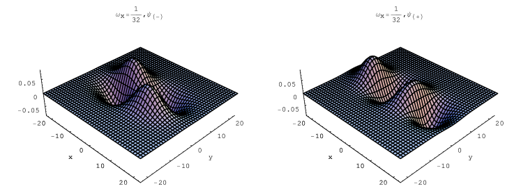
Figure 2: The exact wave functions $\psi_{(\pm)}$ corresponding to the degenerate level of the relative motion energy $\varepsilon^{\textbf{r}}={13\over 32}$

.

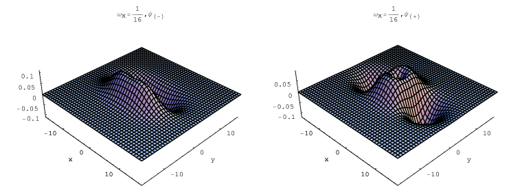
Figure 3: The exact wave functions $\psi_{(\pm)}$ corresponding to the degenerate level of the relative motion energy $\varepsilon^{\textbf{r}}={11\over 16}$

4 Fröbenius method

Now we develop a numerical scheme based on the Fröbenius method (FM) for obtaining the approximate energies of an asymmetric QD (8) in the integrable case of $\omega_{y}:\omega_{x}=2$. The method consists of expanding the solution of a differential equation into power series [19], and was originally applied by Barakat and Rosner [13] to compute the spectrum of one-dimensional quartic oscillator confined by impenetrable walls at $x=\pm R$. The energy eigenvalues of the system have been obtained numerically as zeros of a function, calculated from its power series representation. Moreover, it has been shown that the bound-state energies of the confined system approach rapidly those of the unconfined oscillator for increasing $R$ [13, 14, 15]. Here we show that solving the two separated equations (12) with the help of the power series representation (15) simultaneously with the condition $\beta_{1}+\beta_{2}=2$ enables us to determine effectively the energy levels of the QD to very high precision. With the boundary conditions imposed on the functions $g_{j}(\eta_{j})$ at the points $\eta_{j}=R$, namely $g(R,\beta_{j})=0$, the above problem reduces to finding common zeros $[\delta,\varepsilon^{\textbf{r}}]$ of the functions $g(R,1+\delta)$ and $g(R,1-\delta)$. The functions $g(R,1\pm\delta)$ can be calculated numerically with an arbitrary accuracy from the power series representations

$$g(\eta_{j},\beta_{j})=\sum_{i=0}^{K}b_{i}^{(j)}\eta_{j}^{2i+\nu},$$ (26)

truncated at a suitably high order $K$. The obtained approximations to $g(\eta_{j},\beta_{j})$ are polynomials in the variables $\varepsilon^{\textbf{r}}$ and $\delta$, which can be taken to advantage in determining the numerical values of their common zeros. Since the exact bound-states of the QD correspond to the functions $g(\eta_{j},\beta_{j})$ that vanish at $\eta_{j}\rightarrow\infty$, we expect the solution of the parabolically confined problem to approach the desired solution of the unconfined system, as the confinement range $R$ increases. For the demonstration of convergence, we apply the above scheme to the QD with $\omega_{x}=1/16$, for which the exact solution is known (see Table 1). Table 2 shows how the numerical values $[\delta,\varepsilon^{\textbf{r}}_{FM}]$, obtained for the confined system, approach the exact ones, as the truncation order $K$ in the power series (26) and the confinement range $R$ increase.

Table 2: Convergence of the energy eigenvalue and the corresponding separation constant determined by the FM. The underlined numbers agree with the exact results.

$K$	$R$	0$\varepsilon^{\textbf{r}}_{FM}$	$\hbox{\phantom{\footnotesize\rm 0}}\delta$
60	5	00.6874432520	00.999811134
70		00.6875024844	01.000007959
90	5.5	00.6875000837	01.000000296
100		00.6875000006	01.000000002
120		00.6875000008	01.000000003
140	6	00.6875000000	01.000000000

We have also applied the FM for determining the precise values of energies for the states that are not amenable to exact solution at various $\omega_{y}:\omega_{x}=2$. The stability of numerical results was achieved by increasing $K$ and $R$ until the energy $\varepsilon^{\textbf{r}}_{FM}$ and the corresponding separation eigenvalue $\delta$ stay fixed to the quoted accuracy, which determines the energy of the relative motion of a QD to that accuracy. The bound-state energies determined by the FM are listen in Table 3 up to 8-digit accuracy at particular values of $\omega_{x}$. The states for which the exact solution exists are marked bold, their energies can be shown to agree with the exact values to practically unlimited accuracy. The plot of ground state energy in function of Ln$\omega_{x}$ is displayed in Fig. 4, where we have marked a few of exact values of energy, which correspond to the closed-form solutions discussed in the previous Section.

We may notice that the other integrable case, that of circular symmetry, where the problem reduces to the radial equation for the relative motion, can be also treated within the FM. In that case the solutions has a generalized power series representation and the highly accurate values of energies can be determined with a small computational effort by the scheme developed recently in our previous work [16].

Table 3: Low-lying bound-state energies at various confinement frequencies $\omega_{x}$, as determined by the FM. The existing exact solution are marked bold.

$\omega_{x}$	$\hbox{\phantom{\footnotesize\rm 0}}\varepsilon^{\textbf{r}(+,+)}_{FM}$	$\hbox{\phantom{\footnotesize\rm 0}}\varepsilon^{\textbf{r}(-,+)}_{FM}$	$\hbox{\phantom{\footnotesize\rm 0}}\varepsilon^{\textbf{r}(+,+)(+,-)}_{FM}$	$\hbox{\phantom{\footnotesize\rm 0}}\varepsilon^{\textbf{r}(-,-),(-,+)}_{FM}$
1/64	0.17187500	00.172678376	00.220586977	00.225979324
1/32	0.293674143	00.297716776	00.386949414	00.40625000
1/24	0.367590598	00.37500000	00.490314824	00.521041536
1/16	0.505362736	00.521827040	0 0.68750000	00.743921450
1/8	0.87500000	00.931629324	01.241576361	01.386478626
1/6	1.100931183	01.191668135	01.595014888	01.803819570
1/2	2.681851499	03.142358616	04.266819742	0 5.035425098
1	4.773351606	05.921649105	08.099126926	09.762556072
2	8.623556558	11.317113654	15.569391839	19.083841664

Figure 4: The relative motion ground state energy $\varepsilon^{\textbf{r}}$ of a QD as a function of Ln$\omega_{x}$($\omega_{y}:\omega_{x}=2$) determined by the FM. A few values of energy, for which closed-form solutions exist are marked with crosses.

On the example of a QD with confinement frequency $\omega_{x}={1\over 64}$, we use the exact ground-state energy and the very precise numerical values for higher bound-states determined by the FM (see Table 3) to check the convergence of the popular numerical methods applied directly to the two dimensional Schrödinger equation (8). First, we consider the Rayleigh-Ritz (RR) method with the basis set of the two dimensional harmonic oscillator eigenstates, calculating the approximate values of energies by separate diagonalization of the matrix Hamiltonian corresponding to the eigenfunctions with definite $(x,y)-$parity in a manner similar to that used in Ref. [11]. In Table 4 the obtained values of energies $\varepsilon^{\textbf{r}}_{RR}$ are presented for increasing dimension $D$ of the RR matrix. The same QD example is used for testing the DVR (discrete variable representation) method with the trigonometric basis for the square grid on a square whose sides have length $R$; $x_{i}=y_{i}=-R+2Ri/N,i=1,...,N-1$ (for details see [20]). The numerical values of energies $\varepsilon^{\textbf{r}}_{DVR}$ obtained by diagonalization of the Hamiltonian matrix in point grid representations with dimension $d=(N-1)^{2}$, are presented in Table 5 for several values of $R$ and $d$. We may see that in both considered methods, the rough values of energies can be determined with the use of small basis sets but the convergence is rather slow although the computational effort increases quadratically with the size of the basis.

Table 4: Convergence of low-lying states energy eigenvalues calculated by the Rayleigh-Ritz method for a QD with $\omega_{x}=1/64$. The underlined numbers agree with the exact result or that determined by the FM.

$D$	$\hbox{\phantom{\footnotesize\rm 0}}\varepsilon^{\textbf{r}(+,+)}_{RR}$	$\hbox{\phantom{\footnotesize\rm 0}}\varepsilon^{\textbf{r}(-,+)}_{RR}$	$\hbox{\phantom{\footnotesize\rm 0}}\varepsilon^{\textbf{r}(+,+)}_{RR}$	$\hbox{\phantom{\footnotesize\rm 0}}\varepsilon^{\textbf{r}(+,-)}_{RR}$	$\hbox{\phantom{\footnotesize\rm 0}}\varepsilon^{\textbf{r}(-,-)}_{RR}$	$\hbox{\phantom{\footnotesize\rm 0}}\varepsilon^{\textbf{r}(-,+)}_{RR}$
$25$	00.1718911	00.1726898	00.2206744	00.2206004	00.2259834	00.2260368
$64$	00.1718856	00.1726830	00.2206472	00.2205919	00.2259803	00.2259999
$144$	00.1718823	00.1726804	00.2206274	00.2205891	00.2259796	00.2259878
$256$	00.1718805	00.1726795	00.2206169	00.2205881	00.2259795	00.2259839

Table 5: Same as in Table 4 but calculated by the DVR method.

$d$	0$R$		0	$\hbox{\phantom{\footnotesize\rm 0}}\varepsilon^{\textbf{r}}_{DVR}$	0
$256$	30	00.1719120	00.1727763	00.2206480	00.2214837	00.2260438	00.2277602
$400$		00.1719294	00.1727757	00.2206258	00.2215710	00.2260337	00.2277544
	35	00.1718335	00.1726833	00.2204264	00.2206146	00.2259909	00.2260835
$576$		00.1718460	00.1726824	00.2204845	00.2205998	00.2259843	00.2260752
$900$		00.1718557	00.1726815	00.2205324	00.2205924	00.2259816	00.2260703
	40	00.1718483	00.1726799	00.2204538	00.2205956	00.2259819	00.2259880

5 Concluding remarks

We discussed the case of a QD consisting of two interacting electrons confined in an anisotropic harmonic potential $V(x,y)={m_{*}}(\omega_{x}^{2}{x}^{2}+\omega_{y}^{2}{y}^{2})/2$. In the case of $\omega_{y}:\omega_{x}=2$ we developed a numerical scheme based on the Fröbenius method that allows an efficient determination of the spectrum. Moreover, we have shown that a closed-form analytical solutions for the relative motion can be obtained at particular values of $\omega_{x}$. We illustrated using both the exact and the very precise values of energies determined by FM for testing the convergence of the Rayleigh-Ritz and DVR approximation methods. We have shown that both the methods determine well the approximate values of low-lying states energies but their convergence rates are quite slow.

The exact values of energies and the corresponding wave functions obtained in our work can be useful for investigating the performance of other approximation methods in the case of the asymmetric confinement. They can be also used to build the exact density functional and testing the possible ways of constructing approximations to it.

References

References

- [1] D.J.Thouless, The Quantum Mechanics of many-body systems, Academic Press Inc., New York 1961 and the references therein.
- [2] L. Jacak, P. Hawrylak, and A. Wojs, Quantum Dots (Springer,Berlin ,1997)
- [3] N. S. Simonović and R. G. Nazmitdinov, Phys. Rev.B 67, 041305(R) (2003)
- [4] S.Kais, D.R.Herschbach, and R.D.Levine, J.Chem.Phys. 91, 7791 (1989)
- [5] M. Taut, Phys.Rev. A 48, 3561 (1993)
- [6] W.Zhu and S. B. Trickey, Phys. Rev.A 72, 022501(2005)
- [7] U. Merkt, J.Huser, M.Wagner, Phys.Rev. B 43, 7320 (1991)
- [8] J.L.Zhu, Phys. Rev.B 55, 15 819(1997)
- [9] R. M. G. Garcia-Castelán, W.S.Choe, and Y.C.Lee, Phys.Rev. B 57, 9792 (1998)
- [10] M. Taut, J. Phys. A 27, 1045 (1994)
- [11] P. S. Drouvelis, P. Schmelcher and F. K. Diakonos, Phys. Rev.B 69, 035333(2004)
- [12] P. S. Drouvelis, P. Schmelcher and F. K. Diakonos, Phys. Rev.B 69, 155312(2004)
- [13] R.Barakat, R.Rosner, 1981 Phys.Lett. A83,149
- [14] H.A. Alhendi, E.I. Lashin, J.Phys A:Math.Gen.38 (2005) 6785
- [15] H.A. Alhendi, E.I. Lashin, Can.J.Phys. 83 (2005)541
- [16] P.Kościk and A.Okopińska, J. Phys. A: Math. Gen. 38 (2005) 7743
- [17] A.J. Zakrzewski, Comput.Phys.Comm. 175(2006)397-403
- [18] A.V.Turbiner, Commun.Math.Phys.118(1988)467
- [19] G.B. Arfken, and H.J. Weber, Mathematical Methods of Physicists, Orlando, FL: Academic Press, pp. 462-463, 1985.
- [20] D.T.Colbert and W.H.Miller, (1992) J.Chem.Phys. 9 1982