Ex-house 2D finite-element simulation of the whispering-gallery modes of axisymmetric electromagnetic resonators

Abstract

It is described, explicitly, how a popular, commercially-available software package for solving partial-differential-equations (PDEs), as based on the finite-element method (FEM), can be configured to calculate the frequencies and fields of the whispering-gallery (WG) modes of axisymmetric dielectric resonators. The approach is traceable; it exploits the PDE-solver’s ability to accept the definition of solutions to Maxwell’s equations in so-called ‘weak form’. Associated expressions and methods for estimating a WG mode’s volume, filling factor(s) and, in the case of closed(open) resonators, its wall(radiation) loss, are provided. As no transverse approxi-mation is imposed, the approach remains accurate even for so-called quasi-TM and -TE modes of low, finite azimuthal mode order. The approach’s generality and utility are demonstrated by modeling several non-trivial structures: (i) two different optical microcavities [one toroidal made of silica, the other an AlGaAs microdisk]; (ii) a 3rd-order microwave Bragg cavity containing alumina layers; (iii) two different cryogenic sapphire X-band microwave resonators. By fitting one of the latter to a set of measured resonance frequencies, the dielectric constants of sapphire at liquid-helium temperature have been estimated.

I Introduction

Experimental data are related to physical laws, expressed as equations, through models. To determine the either fundamental, phenomenological, or ‘materials’ constants that the model’s equations include, the model must first be solved, and explicitly so, to allow the fitting of its constants, through (Bayesian) regression, to the experimental data. The inaccurate solution of a model can sometimes contribute significantly to, if not wholly dominate, the fitted values’ uncertainties. Improvements in the accuracies of solutions can alone motivate the (re-)determinations of constants from extant (i.e. ‘old’) experimental data. Indeed, the method of solution presented in this paper’s section II is subsequently exploited, in section VI, to determine the values of certain dielectric constants from the frequencies at which an electromagnetic resonator was found to resonate experimentally; here, the ‘modeling errors’ dominate over other uncertainties.

Once all relevant physical constants are known to sufficient accuracy, a model’s solution can be exploited in the reverse sense to simulate as-yet unrealized experimental embodiments. Simulation enables the properties of a proposed embodiment to be predicted and, thus, through modifications, for its performance (with respect to a given application) to be optimized without, or at least at reduced, experimental effort. Sufficient accuracy in the model’s solution itself is, again, vital. Though analytical models can adequately treat certain highly symmetrical structures, the sufficiently accurate solution of less symmetrical (though more practical) structures typically requires automated numerical computation –as implemented on a digital computer. Here, the model’s structure must first be represented in some ‘electronic’ format. Then, the physical equations, often including sets of partial-differential ones, are encoded and solved for the boundary conditions and constitutive relations that the structure implies. Though these two tasks can be implemented by hand-coding in low-level computer languages, highly developed commercial software packages now exists to facilitate both: (i) computer-aided-design (CAD) tools and (ii) partial-differential-equation (PDE) solvers, respectively. Many, though by no means all [1, 2, 3], of the latter are based on the finite-element method (FEM) [4], which can readily accept CAD-defined structures.

Furthermore, various packages now integrate (i) and (ii) into complete computer-modeling environments, e.g. ‘ECAD’ for simulating electromagnetic systems. These environments sport various additional features for accelerating the definition of models and for facilitating the display and analysis (‘post-processing’) of solutions; they also impose standardized formats and provide (‘house-keeping’) tools to assist in the maintenance, sharing and documentation of a model –so that others can subsequently benefit from, and build upon, the original model-developer’s effort. Compared to the laborious coding up and piecing together of the equivalent software by hand (e.g. as straight MATLAB or Fortran code, making calls to optimized ‘canned’ matrix eigensolvers), the use of such environments, despite their costs and limitations, is attractive.

A problem associated with the inclusion of a complex model into the determination of a constant, where the model is solved via a piece of commercial ‘black-box’ software, or through a proprietary ‘in-house’ service, is that the determination may thus cease to be traceable. Significant effects (or ‘undocumented features’) imparted by the modeling/simulation process may become difficult if not impossible to isolate, understand, or quantify. With regard to traceability, both the model’s definition and its chosen method of solution must remain amenable to explicit representation, thus communication, thus external scrutiny. Convenience and/or efficiency demand, furthermore, that this representation be as concise and elegant as possible –with no ambiguities.

I-A Whispering-gallery-mode resonators

Electromagnetic structures that support whispering-gallery (WG) modes are technologically important because of the advantageous properties that these modes exhibit in terms of spatial compactness, frequency control (either stability or agility) and mode quality ($Q$) factor. Explicit examples will be presented and/or referenced in due course. Compared to the abrupt retro-reflection of an electromagnetic wave at the surface of a mirror, the continuous bending of the same by a whispering-gallery waveguide is an alternative, and at that a still relatively underdeveloped one, which is opening up new applications. Here, one is often interested in a ‘resonator’ where the wave’s trajectory closes back on (and the wave thereby interferes with) itself. Though elliptical [5], helical, or even more complex bending trajectories [6] can be (and have been) envisaged in association with the various morphologies of electromagnetic waveguide/resonator that support WG waves, the author restricts himself here to the study of the simplest, and to-date most popular, class of WG-mode resonator: that where the electromagnetic wave’s trajectory is a plane circle (thus constant radius of curvature) and the electromagnetic structure supporting it is axisymmetric (and coaxial with respect to the said circle/WG mode). Within this class, a convex dielectric:vacuum boundary is often the curved interface of choice for guiding/confining the whispering gallery mode around in an circle. The method presented below can, however, also be employed to simulate WG-modes that are guided by a concave dielectric:metal boundaries. In general then, one considers an axisymmetric toroidal volume, whose cross-section in a (it matters not which) radial-axial plane comprises regions of dielectric (voids correspond to the dielectric vacuum) that are bounded (either externally or from within) by metal surfaces; see FIG. 1.

Despite the breadth and technological allure of this class of WG-mode resonator, it is the author’s understanding that most if not all commercial (ECAD) packages available at the time of writing (early to mid. 2006) suffer from a rather unfortunate ‘blind spot’ when it comes to calculating, efficiently (hence accurately), the whispering-gallery modes (with plane circular trajectories) that such axisymmetric resonator’s support. The popular MAFIA/CST package [7], with which the author is familiar, is a case in point: As has also been experienced by Basu et al [8], and no doubt others, one simply cannot configure the software to take advantage of the WG modes’ apriori-known azimuthal dependence, viz. $\textrm{exp}(\textrm{i}M\phi)$, where $M$ is a positive integer known as the mode’s azimuthal mode order, and $\phi$ is the azimuthal coordinate. Though frequencies and field-patterns can be obtained (at least for WG modes of low azimuthal mode order), the computationally advantageous reduction of the problem from 3D to a 2D that the rotational symmetries of the resonator and its solutions allow is, consequentially, precluded; and the ability to simulate high-order whispering-gallery modes with sufficient accuracy for metrological purposes is, exasperatingly, lost. About the best one can do is to simulate a ‘wedge’ [over an azimuthal domain $\Delta\phi=\pi/(2M)$ wide] between radial electric and magnetic walls [9].

From ECAD to ‘omni-CAD’: Adding titillation to the exasperation, several commercial packages [10, 11] based on the FEM method are now beginning to offer true ‘multiphysics’ capabilities: not only can one separately model a resonator’s electromagnetic response, its mechanical response, its thermal response, …, all based on a common, defined-once-and-for-all geometric structure, one can furthermore couple/‘extrude’/integrate these responses to model non-linear and/or parametric effects. These effects include (as illustrative examples): (i) the electromagnetic heating of a resonator’s lossy dielectrics and/or it resistively conducting inner surfaces (thus shifts in the frequencies of the resonator’s electromagnetic modes), and –even– (ii) ‘mechanical-Kerr’ instabilities/oscillations associated with the mechanical deformation of the resonator’s components due to radiation pressure [12], as exerted by a driven electromagnetic mode. This nirvana of predictive (+ deductive) capability is, for WG-mode resonators, in view of the alluring applications associated with their nonlinear and/or parametric effects, a particularly tantalizing destination –if only one could appropriately configure the (in-the-first-place sufficiently configurable) software to get there. This paper provides a single, though –one might claim– a quite fundamental, generic, and enabling, step on the long march there to.

I-B Brief, selected history of WG-mode simulation

The analysis and modeling of the whispering-gallery modes of electromagnetic resonators, at both optical and microwave frequencies, continues to support and guide experimental endeavor [13, 14, 15, 16]. A brief and far-from-comprehensive survey of the different methods used to implement these simulations to date, with a strong selective bias towards those that have been applied to the study of microwave dielectric-ring resonators, is provided here. The author encourages the reader to consult the earlier works that are referenced within the papers cited below.

Based on ‘separating the variables’ (SV), textbooks [17, 18] provided expressions for the whispering-gallery modes that are supported by whole dielectric parallelopipeds, right-cylinders, and spheres, or dielectric layers and shells exhibiting the same symmetries thereof, where the dielectric volume is enclosed by electric and/or magnetic walls. Illustrating the genre is Wilson et al’s handy study of the transverse electric (TE) and transverse-magnetic (TM) modes of right-cylindrical metal cavities [19], which was in fact used by the author to validate the weak-form expressions described in sub-section II-A below in the early stages of his work.

By ‘mode-matching’ (MM) these SV-solutions across boundaries, WG-mode solutions for composite axisymmetric structures, such as a dielectric right cylinder, surrounded immediately by a void, enclosed within a (coaxial) right-cylindrical metallic jacket (i.e., a so-called ‘can’), can be derived [20, 21]. These solutions, with their associated discrete/integer indices (related to symmetries), provide a nomenclature [22] for classifying WG modes. This nomenclature can be re-used to sort and label the lower-order WG modes of less symmetrical though structurally similar resonators, where these modes can only be calculated ‘blindly’ through other, more numerical methods. Mode-matching by taking linear combinations of several/many –as opposed to just a few– basis functions can increase the ‘fit’ hence accuracy of the MM-SV method and/or allow it to be extended it to the treatment of deformed structures.

In view of the limited computational effort that these semi-analytical SV-based methods demand, remarkable accuracies can be achieved, especially when the most ‘sympathetic’ basis functions are deployed. For many resonators of interest, however, and the composite axisymmetric structures mentioned in the previous paragraph are a case in point, it is not possible, in the MM-SV method (as based on a finite set of basis functions), to simultaneously match all components of the electric and magnetic fields across all boundaries [15] –to do so would, after all, amount to an exact solution! With a small, finite basis set, the ‘transverse’ (or ‘axial-polarization’) approximation, that tolerates a mis-match of ‘minor’ field components, whilst consistently matching the major ones, is uncontrolled. Though extensions to mode-matching that capture spatially non-uniform polarization can be constructed [3], the MM-SV method in general needs to be validated, for a given shape of resonator and mode, through comparison with (more exact) solutions supplied by other methods.

For a complete, accurate solution of Maxwell’s equations, one must generally resort to wholly numerical methods, of which there are several relevant classes and variants. Apart from the finite-element method (FEM) itself (considered in more detail further on), the most developed and thus most immediately exploitable alternatives include (given here for reference –not considered in any greater detail): (i) the Ritz-Rayleigh variational or ‘moment’ methods [23, 24, 25], (ii) the finite difference time domain method (FDTD) [1, 26], and (iii) the boundary-integral [2] or bounday-element methods (BEM, including FEM-based hybridizations thereof [27]). Zienkiewicz and Taylor [4], though nominally dedicated to FEM, provide a taxonomy (viz. table 3.2 loc. cit.) covering most of these methods, which reveals certain commonalities between them. It is remarked here, for example, that FDTD may be regarded as a variant of the FEM employing local, discontinuous shape functions. In conjunction with these generalities, it is worth re-iterating here that the core formulation presented in this paper (viz. equations 8 through 23) can exploit any PDE-solver (e.g. a moment-method-based one) capable of accepting/intepreting weak-form statements. Though a FEM-based solver (viz. COMSOL/FEMLAB) was indeed used to provide the examples presented in section V below, this article’s formulation is not, per se, wedded to FEM.

Though the finite-element method can solve for all field components (both major and minor), the explicit, direct statement of the required set of a coupled partial differential equations (i.e. Maxwell’s equations for WG-mode electromagnetic resonators) in component form, suitable for the insertion into a standard commercial FEM/ECAD software package, can be extremely onerous –if not absolutely ruled out by the software’s lack of configurability. This is why the majority of these packages already include pre-defined ‘applications modes’, ‘macros’ or ‘wizards’ for solving electromagnetic problems (for particular geometries). To simplify the problem to that of a single (scalar) PDE, one can again [cf. the SV-MM method(s) already discussed above] invoke the so-called transverse (axial-polarization) approximation, where the resonator’s either magnetic or electric field is forced to lie everywhere parallel to the resonator’s axis of rotational symmetry; figure B.1 of reference [28] displays this approximation most pedagogically. Investigations based on this ‘transverse-FEM’ approach have been reported in several recent works [8, 28]. Though it can provide indicative trends and quantitative results, which might well be sufficiently accurate and/or robust for the calculation’s intended purpose (in view of even less well controlled experimental parameters), the uncontrolled nature of the approximation that transverse-FEM incorporates is again far from ideal. The careful physicist, or metrologist, is (again) compelled to justify its validity, for a given resonator and mode, through comparison with either non-trivial analytical solutions, where they exist, or ‘brute force’ (3D) numerical computation [8]. It is this paper’s principal claim that, through only a modicum of extra effort, the transverse approximation, and its associated onerous validations [or (else) lingering doubts], can be wholly obviated.

The application of the finite-element method to the solving of Maxwell’s equations has a history [29], and is now very much an industry [7, 10, 11]. Zienkiewicz and Taylor [4] supply FEM’s theoretical underpinnings, in particular an erudite account of Galerkin’s method of so-called ‘weighted residuals’. A pervasive, and often quite debilitating problem that besets the direct/‘naïve’ applications of FEM to the PDEs that are Maxwell’s equations is the generation of (a great many) spurious solutions [30, 31], associated with the local gauge invariance, or ‘null space’ [31], which is a (hidden) feature of these PDEs (in particular its ‘curl’ operators). At least two research groups have nevertheless successfully developed software tools for calculating the WG modes of axisymmetric dielectric resonators, where these tools (i) solve for all field components (i.e. no transverse approximation is invoked), (ii) are 2D (and thus numerically efficient) and (iii) effectively suppress spurious solutions (without any insidious, detrimental side-effects) [30, 23, 24, 32, 33]. The method reported below sports these same three attributes. With regard to (iii), the approach adopted by Auborg et al was to use different finite elements (viz. a mixture of ‘Nedelec’ and ‘Lagrange’ -both 2nd order) for different components of the electric and magnetic fields; Osegueda et al [32], on the other hand, used a so-called ‘penalty term’ to suppress (spurious) divergence of the magnetic field. Stripping away all of its motivating remarks, applications and illustrations, the principal function of this paper is to convert (one might say ‘extract’) the method encoded by Osegueda et al’s ‘CYRES’ 2D FEM software package [32] into explicit ‘weak-form’ expressions, that can be directly and openly ported to any PDE solver (most notably COMSOL/FEMLAB) capable of accepting such. These weak-form expressions are wholly equivalent to the Maxwellian PDEs from which they are derived. But, being scalar (tensorially-contracted), they are considerably less onerous to represent and communicate than the vectorial PDEs themselves. The author hopes that, by stating/popularizing the problem so explicitly in this paper through the lingua franca of weak form, the means to model, both accurately and traceably, the whispering-gallery modes of axisymmetric resonators will thereby be made accessible to any competent engineer or physicist in need of such a means –‘off the shelf’, as opposed to it remaining a strictly ‘in-house’ (and thus rather less open and traceable) capability retained by specialists.

II Method of solution

II-A Weak forms

Scope: The types of ideal resonator that fall under the scope of the analysis presented immediately below are those that comprise volumes of lossless dielectric space bounded by a combination of perfect (thus also loss-less) electric or magnetic walls –see Fig. 1 (though note that the restriction to resonators of axisymmetric form needs only to be invoked at the start of subsection II-B).

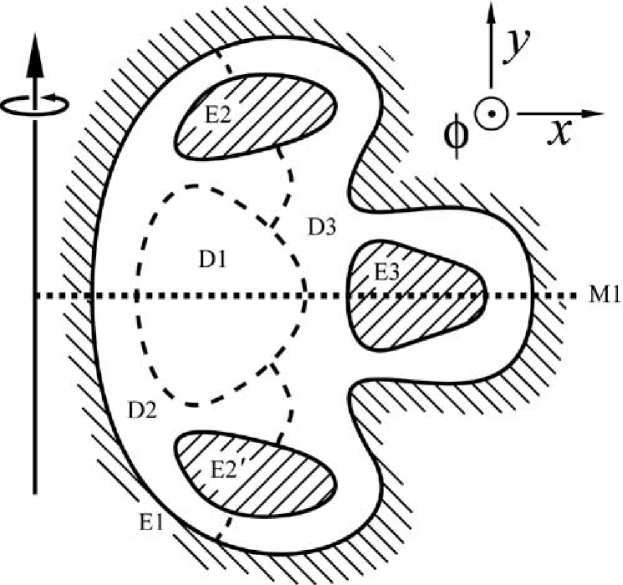
Figure 1: Generic axisymmetric resonator in cross-section (medial half-plane). A dielectric region enclosed by an electric wall E1 is subdivided into subdomains D1, D2 and D3, none, one or more of which could be free space. D2 and D3 are bounded internally by electric walls E2, E2^′ and E3. The resonator’s mirror symmetry through the horizontal (equatorial) plane, as indicated by the dashed line M1, allows an additional either electric or magnetic wall to be placed on it and, thereupon, only one half of the resonator’s domain (either its upper or lower half) need be simulated.

As discussed in subsections III-D through IV-B below, a dissipative (open) resonator’s finite fractional energy loss per cycle, hence its sub-infinite $Q$-factor, can be estimated, and with often perfectly sufficient accuracy with regard to applications, from the solution of an equivalent loss-less (closed) resonator. The resonator’s dielectric space will, in general, comprise both voids (i.e. the free space of a vacuum) and space filled by sufficiently ‘good’ (i.e. low-loss) dielectric material(s). A model’s electric walls will translate, in embodiments, to metallic surfaces whose conductivities are sufficiently good to be treated as such (section III-D quantifies the loss caused by the metallic wall of a particular resonator’s can). The (relative) permeability of real magnetic materials is seldom high enough for a wall made from such to be regarded, without deleterious approximation, as a (perfect) magnetic one. When modeling resonators whose forms exhibit reflection symmetries, such that the magnetic and electric fields of their solutions exhibit either symmetry or antisymmetry through mirror planes, perfect magnetic and electric walls can be advantageously imposed on the model’s mirror plane to solve for particular ‘sectors’ of solutions.

The electromagnetic field within the dielectric volumes of the resonator obeys Maxwell’s equations [34, 18], as they are applied to continuous, macroscopic media [35]. Thus, on the assumption that the resonator’s constituent dielectric elements have negligible (or at least the same) magnetic susceptibility (hence permeability), the magnetic field strength H is continuous across all interfaces between them. This property makes it advantageous to solve for H (or the magnetic flux density $\textbf{B}=\mu\textbf{H}$ related to it by a constant global magnetic permeability $\mu$), as opposed to the electric field strength E (or displacement D). Upon substituting one of Maxwell’s ‘curl’ equations equations into the another, the problem reduces to that of solving the (modified) vector Helmholtz equation

$$\boldsymbol{\nabla}\boldsymbol{\times}({\boldsymbol{\epsilon}^{-1}}\;\boldsymbol{\nabla}\boldsymbol{\times}\textbf{H})-\alpha\boldsymbol{\nabla}(\boldsymbol{\nabla}\cdot\textbf{H})+c^{-2}\partial^{2}\textbf{H}/{\partial t^{2}}=0$$ (1)

subject to appropriate boundary conditions (read on), where $c$ is the speed of light. Here, ${\boldsymbol{\epsilon}^{-1}}$ denotes the inverse relative permittivity tensor; one assumes that the resonator’s dielectric elements are linear, such that it is a (tensorial) constant –i.e. independent of field strength. The middle (penalty) term on the left-hand side of equation 1 is the same as that used by Osegueda et al [32]; it functions to suppress/reveal spurious modes in the finite-element simulation; the constant $\alpha$ controls this term’s weight with respect to its Maxwellian neigbours. The penalty term’s insertion into the above Helmholtz equation is wholly permissible since, for every true solution of Maxwell’s equation, it must exactly vanish (everywhere): the magnetic flux density B, hence (for non- or isotropically-magnetic media) $\textbf{H}=\textbf{B}/\mu$, is required to be free of divergence –assuming no magnetic monopoles lurk inside the resonator.

Reference [18] (particular section 1.3 thereof) supplies a primer on the electromagnetic boundary conditions discussed forthwith. Assuming that the resonator’s bounding electric walls are perfect in the sense of having (effectively) infinite surface conductivity, the magnetic flux density at any point on each such wall is required to satisfy $\textbf{B}\cdot\textbf{n}=0$, where n denotes the wall’s surface normal vector. Providing the magnetic permeability/susceptibility of the dielectric medium bounded by the electric wall is not anisotropic, this condition is equivalent to

$$\textbf{H}\cdot\textbf{n}=0.$$ (2)

The electric field strength at the electric wall is required to obey

$$\textbf{E}\boldsymbol{\times}\textbf{n}=0;$$ (3)

these two equations ensure that the magnetic (electric) field strength is oriented tangential (normal) to the electric wall. As is pointed out in reference [32], equation 3 is a so-called ‘natural’ (or, synonymously, a ‘naturally satisfied’) boundary condition within the finite-element method –see ref. [4].

When the resonator’s form (hence those of its solutions) exhibits one or more symmetries, it is often advantageous (for reasons of computational efficiency) to solve only for a symmetry-reduced portion or ‘sector’ of the full resonator, where this sector is bounded by either (real or virtual) electric walls or (virtual) magnetic walls, or both. The boundary conditions corresponding to a perfect magnetic wall (dual to the those for an electric wall) are

$$\textbf{D}\cdot\textbf{n}=0,$$ (4)

and

$$\textbf{H}\boldsymbol{\times}\textbf{n}=0;$$ (5)

these two equations ensure that the electric displacement (magnetic field strength) is oriented tangential (normal) to the magnetic wall. Again, the latter equation is naturally satisfied.

One now invokes Galerkin’s method of weighted residuals; reference [4] explains the fundamentals here; reference [31] provides an analogous treatment when solving for the electric field strength (E). Both sides of equation 1 are multiplied (scalar-product contraction) by the complex conjugate of a ‘test’ magnetic field strength $\tilde{\textbf{H}}^{*}$, then integrated over the dielectric resonator’s interior volumes. Upon expanding the permittivity-modified ‘curl of a curl’ operator (to extract a similarly modified Laplacian operator), then integrating by parts (spatially), then disposing of surface terms through the electric- or magnetic-wall boundary conditions stated above, one arrives (equivalent to equation (2) of reference [32]) at

$$\int_{\textrm{V}}[(\boldsymbol{\nabla}\boldsymbol{\times}\tilde{\textbf{H}}^{*})\;\frac{\cdot}{\boldsymbol{\epsilon}}\;(\boldsymbol{\nabla}\boldsymbol{\times}\textbf{H})-~{}~{}~{}~{}~{}~{}~{}~{}~{}~{}\\ \;\alpha(\boldsymbol{\nabla}\cdot\tilde{\textbf{H}}^{*})(\boldsymbol{\nabla}\cdot\textbf{H})+c^{-2}\tilde{\textbf{H}}^{*}\cdot\partial^{2}\textbf{H}/{\partial t^{2}}]\,\textrm{d}\textrm{V}=0,$$ (6)

where ‘$\int_{\textrm{V}}$’ denotes the volume integral over the resonator’s interior space (or sector thereof) and ‘$\cdot/\boldsymbol{\epsilon}$’ denotes a contraction weighted by inverse relative permittivities. The three terms appearing in the integrand correspond directly to the three weak-form terms required to define an appropriate finite-element model within the PDE solver.

Assuming that the physical dimensions and electromagnetic properties of the resonator’s components are temporally invariant (or at least ‘quasi-static’), one seeks harmonic or ‘modal’ solutions: $\textbf{H}(\textbf{r};t)=\textbf{H}(\textbf{r})\textrm{exp}(-\textrm{i}2\pi ft)$, where r is the vector of spatial position, $t$ the time, and $f$ the mode’s resonance frequency. The last, ‘temporal’ term in equation 6’s integrand can thereupon be re-expressed as $-(\bar{c}f)^{2}\tilde{\textbf{H}}(\textbf{r})^{*}\cdot\textbf{H}(\textbf{r})$, where $\bar{c}\equiv 2\pi/c$ and $c$ is the speed of light. This re-expression(and, with respect to Spillane et al’s work, using exactly the same FEM software platform) reveals the integrand’s complete dual symmetry between $\tilde{\textbf{H}}^{*}$ and H.

II-B Axisymmetric resonators

One now restricts the scope of the analysis to resonators whose interiors and bounding surfaces are electromagnetically axisymmetric (henceforth referred to simply as ‘axisymmetric resonators’) where a system of cylindrical coordinates is aligned with respect to the resonator’s axis of rotational symmetry. This system’s three components are $\{x,\phi,y\}\equiv$ {‘rad(ial)’, ‘azi(muthal)’, ‘axi(ial)’}. One wishes to calculate the resonance frequencies and field patterns of the resonator’s (standard) whispering-gallery (WG) modes, whose phase varies as $\textrm{exp}(\textrm{i}M\phi)$, where $M=\{0,1,2,...\}$ is the WG mode’s azimuthal mode order. Note that the method does not require $M$ to be large (i.e., it is not an ‘asymptotic’ method); even modal solutions that are themselves axisymmetric, corresponding to $M=0$, such as the one shown in Fig. 6(b), can be calculated. Viewed as a three-component vector field over a (for the moment) three-dimensional space, the time-independent part of the magnetic field strength now takes the form

$$\textbf{H}(\textbf{r})=\textrm{e}^{\textrm{i}M\phi}\left\{\right.H^{x}(x,y),\textrm{i}\,H^{\phi}(x,y),H^{y}(x,y)\left.\right\}$$ (7)

where an ‘i’ ($\equiv\surd(-1)$) has been inserted into the field’s azimuthal component so as to allow, in subsequent solutions, all three component amplitudes $\left\{H^{x},H^{\phi},H^{y}\right\}$ to each be expressible as a real amplitude multiplied by a common complex phase factor. The relative permittivity tensor of an axisymmetric dielectric material is diagonal with entries (running down the diagonal) $\boldsymbol{\epsilon}_{\textrm{diag.}}=\{\epsilon_{\perp},\epsilon_{\perp},\epsilon_{\parallel}\}$, where $\epsilon_{\parallel}$ is the material’s relative permittivity in the axial direction and $\epsilon_{\perp}$ its relative permittivity in the plane spanned by it radial and azimuthal directions.

It now remains only to substitute equation 7 into equation 6’s integrand and express the three terms composing the latter’s integrand in terms of the magnetic field strength’s components (and their spatial/temporal derivatives); textbooks provide the required explicit expressions for the vector differential operators in cylindrical coordinates [36, 17, 18]. A radial factor, $x$, is included here from the volume integral’s measure: $\textrm{d}\textrm{V}=2\pi\,x\,\textrm{d}x\,\textrm{d}\phi\,\textrm{d}y$ (the factor of $2\pi$ here is uniformly, thus inconsequentially, dropped from all three expressions below.) These requisite expansions are presented here in compact mathematically notation; their line-text (i.e. with no super- or sub-scripts, hence considerably more verbose) equivalents, in forms suitable for direct cut-and-paste injection into a popular PDE-solver (viz. COMSOL/FEMLAB) are available as a separate ‘Appendix’ to this paper [37]. The first, ‘Laplacian’ weak term is given by

$$(\boldsymbol{\nabla}\boldsymbol{\times}\tilde{\textbf{H}}^{*})\frac{\cdot}{\boldsymbol{\epsilon}}\;(\boldsymbol{\nabla}\boldsymbol{\times}\textbf{H})=\bigl{(}\frac{A}{x}+B+x\,C\bigr{)}/({\epsilon_{\perp}\epsilon_{\parallel}}),$$ (8)

where

$$A\equiv\{\,\epsilon_{\perp}[\tilde{H}^{\phi}H^{\phi}-M(\tilde{H}^{\phi}H^{x}+H^{\phi}\tilde{H}^{x})+M^{2}\tilde{H}^{x}H^{x})]\\ ~{}~{}~{}~{}~{}~{}+\epsilon_{\parallel}M^{2}\tilde{H}^{y}H^{y}\,\},$$ (9)

$$B\equiv\epsilon_{\perp}[\tilde{H}^{\phi}_{x}(H^{\phi}-MH^{x})+H^{\phi}_{x}(\tilde{H}^{\phi}-M\tilde{H}^{x})]\\ ~{}~{}~{}~{}~{}-\epsilon_{\parallel}M(\tilde{H}^{y}H^{\phi}_{y}+H^{y}\tilde{H}^{\phi}_{y}),$$ (10)

$$C\equiv\{\,\epsilon_{\perp}\tilde{H}^{\phi}_{x}H^{\phi}_{x}\\ ~{}~{}+\epsilon_{\parallel}[(\tilde{H}^{y}_{x}-\tilde{H}^{x}_{y})(H^{y}_{x}-H^{x}_{y})+\tilde{H}^{\phi}_{y}H^{\phi}_{y}]\,\},$$ (11)

where $H^{\phi}_{x}$ denotes the partial derivative of $H^{\phi}$ (the aziumthal component of the magnetic field strength) with respect to $x$ (the radial component of displacement), etc.. Here, the individual factors and terms have been ordered and grouped so as to display the dual symmetry. Similarly, the weak penalty term is given by

$$\alpha(\boldsymbol{\nabla}\cdot\tilde{\textbf{H}}^{*})(\boldsymbol{\nabla}\cdot\textbf{H})=\alpha\{\frac{D}{x}+E+x\,F\},$$ (12)

where

$$D\equiv\tilde{H}^{x}H^{x}-M(\tilde{H}^{\phi}H^{x}+H^{\phi}\tilde{H}^{x})+M^{2}\tilde{H}^{\phi}H^{\phi},$$ (13)

$$E\equiv(\tilde{H}^{x}_{x}+\tilde{H}^{y}_{y})(H^{x}-MH^{\phi})\\ +(\tilde{H}^{x}-M\tilde{H}^{\phi})(H^{x}_{x}+H^{y}_{y}),~{}~{}~{}~{}~{}~{}~{}~{}~{}~{}~{}$$ (14)

$$F\equiv(\tilde{H}^{x}_{x}+\tilde{H}^{y}_{y})(H^{x}_{x}+H^{y}_{y}).~{}~{}~{}~{}~{}~{}~{}~{}~{}~{}~{}~{}~{}~{}~{}~{}~{}~{}~{}~{}~{}~{}~{}~{}~{}~{}~{}$$ (15)

And, finally, the temporal weak-form (‘dweak’) term is given by

$$\tilde{\textbf{H}}^{*}\cdot\partial^{2}\textbf{H}/{\partial^{2}t}=c^{-2}\,x\,(\tilde{H}^{x}H^{x}_{tt}+\tilde{H}^{\phi}H^{\phi}_{tt}+\tilde{H}^{y}H^{y}_{tt})~{}~{}~{}~{}~{}~{}~{}~{}~{}~{}~{}~{}~{}~{}~{}~{}~{}~{}~{}\\ ~{}~{}~{}~{}~{}~{}~{}~{}~{}=-\bar{c}^{2}f^{2}\,x\,(\tilde{H}^{x}H^{x}+\tilde{H}^{\phi}H^{\phi}+\tilde{H}^{y}H^{y}),$$ (16)

where $H^{x}_{tt}$ denotes the double partial derivative of $H^{x}$ w.r.t. time, etc.. What is crucial is that none of the terms on the right-hand sides of equations 8 through 16 depend on the azimuthal coordinate $\phi$; the problem has been reduced from 3D to 2D.

II-C Axisymmetric boundary conditions

An axisymmetric boundary’s unit normal in cylindrical components can be expressed as $\{n_{x},0,n_{y}\}$ –note vanishing azimuthal component. The full electric-wall boundary conditions, in cylindrical components, are as follows: $\textbf{H}\cdot\textbf{n}=0$ gives

$$H^{x}n_{x}+H^{y}n_{y}=0,$$ (17)

and $\textbf{E}\boldsymbol{\times}\textbf{n}=0$ includes both

$$H^{x}_{y}-H^{y}_{x}=0$$ (18)

and

$$\epsilon_{\perp}(H^{\phi}-H^{x}M+H^{\phi}_{x}x)n_{x}-\epsilon_{\parallel}(H^{y}M-H^{\phi}_{y}x)n_{y}=0.$$ (19)

When the dielectric permittivity of the medium bounded by the electric wall is isotropic (which is often the case in embodiments), the last condition reduces to

$$(H^{\phi}-H^{x}M+H^{\phi}_{x}x)n_{x}-(H^{y}M-H^{\phi}_{y}x)n_{y}=0.$$ (20)

The full magnetic-wall boundary conditions, in cylindrical components, are as follows: the condition $\textbf{D}\cdot\textbf{n}=0$ gives

$$(H^{y}M-H^{\phi}_{y}x)n_{x}+(H^{\phi}-H^{x}M+H^{\phi}_{x}x)n_{y}=0,$$ (21)

and the condition $\textbf{H}\boldsymbol{\times}\textbf{n}=0$ includes both

$$H^{y}n_{x}-H^{x}n_{y}=0$$ (22)

and

$$H^{\phi}=0.$$ (23)

One observes that the transformation $\{n_{x}\rightarrow-n_{y},n_{y}\rightarrow n_{x}\}$, connects equations 17 and 22, and equations 20 with 21. Explicit PDE-solver-ready equivalents of 17 through 23 are stated in this paper’s auxiliary Appendix [37]. The above weak-form expressions and boundary conditions, viz. equations 8 through 23 are the key enabling results of this paper: once inserted into a PDE-solver, the WG modes of axisymmetric dielectric resonators can readily be calculated, as is demonstrated for particular embodiments in section V below.

III Postprocessing of solutions

Having determined, for each mode, its frequency and all three components of its magnetic field strength H as functions of position, other relevant fields and parameters can be derived from them.

III-A Remaining Maxwellian fields

Straightaway, the magnetic flux density $\textbf{B}=\textbf{H}/\mu$; here, as stated in subsection II-A above –but see also footnote 4, the magnetic permeability $\mu$ is assumed to be a scalar constant, independent of position. [And for each of the resonators considered in section V, $\mu=\mu_{0}$ everywhere –to an adequate approximation.] As no real (‘non-displacement’) current flows within a dielectric, $\nabla\boldsymbol{\times}\textbf{H}(t)=\partial\textbf{D}(t)/\partial t$, thus $\textbf{D}=-\textrm{i}(2\pi f)^{-1}\nabla\boldsymbol{\times}\textbf{H}(t)$. And, $\textbf{E}=\boldsymbol{\epsilon}^{-1}\textbf{D}$, where $\boldsymbol{\epsilon}^{-1}$ is the (diagonal) inverse permittivity tensor, as already discussed in connection with equation 6 above.

III-B Mode volume and filling factor

Accepting various caveats (most fundamentally, the problem of mode-volume divergence –see footnote 7; and inconsistent definitions between different authors …) as addressed by Kippenberg [28], the volume of a mode in a dielectric resonator is here defined as [14]

$$V_{\rm{mode}}=\frac{\int\int\int_{\rm{h.-s.}}\epsilon|\textbf{E}|^{2}\textrm{d}\textrm{V}}{{\rm{max}}[\epsilon|\textbf{E}|^{2}]},$$ (24)

where ${\rm{max}}[...]$, denotes the maximum value of its functional argument, and $\int\int\int_{\rm{h.-s.}}...\textrm{d}\textrm{V}$ denotes integration over and around the mode’s ‘bright spot’ –where its electromagnetic field energy is concentrated.

III-C Filling factor

The resonator’s electric filling factor, for a given mode, a given dielectric piece/material, $\rm{diel.}$, and a given field direction, ($\rm{dir.}\in\{\rm{radial},\rm{azimuthal},\rm{axial}\}$), is defined as

$$F_{\rm{diel.}}^{\rm{dir.}}=\frac{\int\int\int_{\rm{diel.}}\epsilon_{\rm{pol.}}|E^{\rm{dir.}}|^{2}\textrm{d}\textrm{V}}{\int\int\int\epsilon|\textbf{E}|^{2}\textrm{d}\textrm{V}},$$ (25)

where $\int\int\int_{\rm{diel.}}...\textrm{d}\textrm{V}$ denotes integration only over those domains composed of the dielectric in question and $\rm{pol.}$ = $\{\perp,\parallel\}$ for $\rm{dir.}$ = $\{\rm{radial}\;\rm{or}\;\rm{azimuthal},\rm{axial}\}$. The numerators and denominators of equations 24 and 25 can be readily evaluated using the PDE-solver’s post-processing features.

III-D Finite Qs and wall losses

So far, the model resonator as per Fig. 1 has been treated as a wholly loss-less one: its modal solutions have infinite $Q$s or, equivalently, the (otherwise complex) frequencies of these solutions are purely real or, equivalently, the solutions’ oscillatory electromagnetic fields persist indefinitely. No energy is dissipated by the dielectric material(s) included within the resonator (their dielectric loss tangents are presumed to be zero); none is lost through radiation –since the resonator’s bounding perfect electric/magnetic walls allow none to escape; and, being perfect, the current induced within the wall causes no resistive dissipation.

Real resonators, on the other hand, are subject to one or several dissipative processes, i.e. ‘losses’, that render the $Q$s of resonances finite. This subsection provides an expression for the rate of a resonator’s ‘wall loss’; section IV goes on to provide bounds on the rate of an open resonator’s ‘radiation loss’. Such estimates are important since $Q$ values are directly measurable in experiments and, furthermore, often determine viability and/or performance in applications. The approach taken here is to build upon (via perturbation theory and/or ‘induction’) the loss-less model, as it has already been formulated in section II –as opposed to constructing the additional machinery required to model resonators with lossy materials either placed within or clad about them.

Preliminaries: The space that a WG-mode occupies can be broadly divided into three regions: (i) the mode’s ‘near-field’, which includes its bright spot(s) –where the modes e.m. energy density is greatest, (ii) an ‘evanescent zone’, lying around the near-field, where the mode’s field amplitudes (and energy density) decay exponentially with distance $r$ away from its bright spot and (iii) a (notionally infinite) ‘radiation zone’, lying outside of the evanescent zone (a ‘cusp’ can separate the two), where the field-amplitudes decay as $\sim 1/r$. If a compact, closed resonator of high-$Q$ is sought, its electric (i.e. metal) wall should be placed sufficiently far from the WG-mode’s bright spot in the exponentially decaying zone (ii), but, for reasons of compactness, no further out than is necessary.

A brief word of warning: As the $Q$ of an experimental WG-resonator can be exceedingly high ($>10^{9}$), the amplitude of the electromagnetic field where dominant losses occur (their rates will depend on the amplitude) can be many orders of magnitude lower than the field’s maximum (or maxima) at the WG-mode’s bright spot(s). The hardware and software employed to generate WG-modal solutions must thus be able to cope with such a dynamic range, lest significant numerical errors creep into the predicted (loss-rate-determining) amplitudes where the WG-resonator’s supported mode is faint. In practice, this means adequate-precision arithmetic, adequate mesh densities (with FEM), and, where confidence or experience is lacking, a thorough testing of the robustness of the solution against changes in the geometry or mesh density.

Now, the energy stored in the resonator’s electromagnetic field is $U=(1/2)\int\int\int\mu|\textbf{H}|^{2}\textrm{d}\textrm{V}$, where H is the infinite-$Q$ solution generated by the PDE-solver, and $\mu$ is the common permeability for the resonator’s interior. For resonators that are axisymmetric, the 3D volume integral $\int\int\int\textrm{d}\textrm{V}$ over the resonator’s interior reduces to the 2D integral $\int\int(2\pi x)\textrm{d}x\textrm{d}y$ over its medial cross-section. The surface current induced in the resonator’s enclosing perfect-electric wall is given by (see ref. [18], page 205, for example) $\textbf{J}_{s}=\textbf{H}_{\rm{t}}\equiv\textbf{n}\boldsymbol{\times}\textbf{H}$, where $\textbf{H}_{\rm{t}}$ is the tangential component of H with respect to the resonator’s electric-wall boundary.

One now exploits (first-order) perturbation theory, and equates the current immediately stated above with that which would be induced into the electric walls of a resonator, identical to its loss-less antecedent, but for it having electric walls of finite conductivity. The equating of the two currents assumes that the lossy walls are nevertheless made out of (or coated with) a sufficiently ‘good’ conductor, such that the change from loss-less to lossy does not significantly affect the shapes of the resonator’s modes. This will typically be the case for a cavity resonator exciting low-order modes at microwave frequencies, provided its walls are made from any standard (electrically good) metal, such as copper; again, see references [18] and/or [34] for further explanation/quantification.

The time-averaged(-over-a-cycle) power lost by the resonator through resistive heating in its imperfect electric walls is thereupon given by $P_{\rm{loss}}=(1/2)\int\int R_{s}|\textbf{n}\boldsymbol{\times}\textbf{H}|^{2}\textrm{d}\textrm{S}$, where the 2D surface integral $\int\int\textrm{d}\textrm{S}$ over the resonator’s presumed axisymmetric enclosing boundary reduces to the 1D integral $\int(2\pi x)\textrm{d}\textrm{l}$ around the periphery of its medial (x-y) cross-section; $R_{s}=(\pi f\mu/\sigma)^{1/2}$ is the wall’s surface resistivity, where $\sigma$ is the wall’s (bulk) electrically conductivity, and $f$ the mode’s frequency. The quality factor, defined as $2\pi f\,U/P_{\rm{loss}}$, due to the wall’s resistive losses can thus be expressed as:

$$Q_{\rm{wall}}=\frac{2\pi f\,\mu}{R_{\rm{s}}}\Lambda=(4\pi f\,\mu\,\sigma)^{1/2}\Lambda,$$ (26)

where $\Lambda$, which has the dimensions of a length, is defined as

$$\Lambda=\frac{\int\int\int|\textbf{H}|^{2}\textrm{d}\textrm{V}}{\int\int|\textbf{n}\boldsymbol{\times}\textbf{H}|^{2}\textrm{d}\textrm{S}}\\ =\frac{\int\int[(H^{x})^{2}+(H^{\phi})^{2}+(H^{y})^{2}]\,x\,\textrm{d}x\,\textrm{d}y}{\int x\,[|H^{\phi}|^{2}+|H^{y}dn_{x}-H^{x}n_{y}|^{2}]\rm{dl}}.$$ (27)

Both integrals (numerator and denominator), hence $Q_{\rm{wall}}$ itself, can be readily evaluated using the PDE-solver’s post-processing features; explicit PDE-solver-ready forms of each integrand are provided in this paper’s separate Appendix [37]. In the using of equation 26, it should be pointed out that, at liquid-helium temperatures, the bulk and surface resistances of metals can depend greatly on the levels of (magnetic) impurities within them [38], and the text-book $f^{-1/2}$ dependence of surface resistance on frequency is often violated [39].

IV Radiation Loss in Open Resonators

IV-A Open resonators: preliminary remarks

Many whispering-galley mode resonators (both microwave [40] and optical [12, 14]) of interest experimentally are not shielded by an enclosing metal wall: they are open. In consequence, the otherwise highly localized WG mode supported by the resonator spreads throughout free-space, leading to the conveyance of energy away from the mode’s bright spot (where the electric- and magnetic-field amplitudes are greatest) through radiation. Provided the equivalent closed resonator’s enclosing electric (i.e. metal) wall is stationed sufficiently far out in the WG mode’s evanescent zone, the WG mode’s form in its near-field will be the same (to the degree of equivalence required here) in both the open-resonator and closed-resonator cases. One can thus calculate the mode’s near-field form through the method developed in section II, or by some other method, as applied to the closed resonator; in particular, the electric and magnetic field strengths, E and H or, equivalently, the vector potential A, just outside of the surface(s) of the resonator’s dielectric component(s) can be determined. Having done so, the WG mode’s far-field form (i.e. its ‘radiation pattern’) in the case of the open resonator can be calculated by invoking the so-called Field Equivalence Principle [41, 42], where A or (the tangential components of) E and H over the said surface(s) are regarded, in Huygen’s picture, as (secondary) sources radiating into free-space. The calculation can be implemented through a standard retarded-potential (Green function) approach [17, 42], incorporating (if necessary) a multipole expansion. The mode’s radiative loss, hence $Q$, can be subsequently calculated from the radiation pattern determined by integrating Poynting’s vector over all solid angles. With due care, the resulting estimate of the mode $Q$ will be highly accurate. But such a program of work –for lack of novelty rather than utility– shall not be undertaken here.

IV-B Estimators of radiation loss

Instead, two different (but related) ‘trick’ methods for estimating the radiative $Q$ of an open (dielectric) resonator are described here. As the first method underestimates the $Q$, while the second overestimates it, the two in conjunction can be used to bound the $Q$ from below and above. Moreover, both can be implemented as straightforward ‘add-ons’ to the 2D PDE-solver’s computational environment, as already configured for solving closed loss-less resonators (as per section II). It should be added that these two methods are not restricted to axisymmetric resonators per se.

IV-B1 Underestimator via (imperfect) retro-reflection

Consider an otherwise loss-less open resonator, supporting a spatially concentrated mode, i.e. one with a bright spot, that radiates into free-space. As stated above, the tangential electric and magnetic fields on any closed surface in the near-field surrounding this mode’s bright spot can, by the Field Equivalence Principle, be regarded as a (secondary) source of this radiation. Now consider a closed, completely loss-less equivalent of the open resonator, formed by placing a cavity around it, whose enclosing perfect-electric wall lies in the said localized mode’s radiation zone. It is noted here, for future reference, that this perfect electric wall will force the tangential component of the electric field strength to vanish everywhere on it, i.e. $\textbf{E}-\textbf{n}(\textbf{E}\cdot\textbf{n})=0$, where n is the wall’s unit normal vector. The above-mentioned secondary source generates an outward-going traveling wave wave which, but for the cavity, would lead to radiation. Instead, with the cavity in place, a standing (as opposed to traveling) wave arises. Now, suppose that the shape of the cavity’s electric wall, and its location with respect to the source, is chosen to predominantly reflect the source’s outward-going wave back to the source such that the resultant inward-going wave interferes constructively with the outgoing wave over the whole of the source’s surface. In other words (1D analogy), on regarding the cavity as a short-circuit-terminated transmission line, one attempts to adjust the length of the line such that its input (analogous to the source’s surface) is located at an antinode of the line’s standing wave. If such a retro-reflecting (+ phase-length adjusted) cavity can be devised then, in particular, the measured/simulated tangential magnetic field, $\textbf{H}_{\rm{t}}$, just inside of the cavity’s electric wall will be exactly twice that of the outward-going wave for the open resonator $\textbf{H}_{\rm{t}}^{\rm{rad.}}$ at the same location –but without the cavity’s electric wall in place. In practice, the source will not be located exactly at an antinode (over the whole of its surface) and thus $\textbf{H}_{\rm{t}}>2\textbf{H}_{\rm{t}}^{\rm{rad.}}$. The radiative loss for the open resonator can be evaluated by integrating the cycle-averaged Poynting’s vector corresponding to the outward-going wave’s inferred tangential magnetic field over the electric wall’s surface; i.e. $P_{\rm{rad.}}=(1/2)\int\int z_{0}|\textbf{H}_{\rm{t}}^{\rm{rad.}}|^{2}\textrm{d}\textrm{S}$, where $z_{0}$ is the impedance of free space. A bound on the open resonator’s radiative $Q$-factor can thus be expressed as

$$Q_{\rm{rad.}}>(8\pi f/c)\Lambda,$$ (28)

where $\Lambda$ is exactly that given by equation 27 but with the (loss-less) electric wall now in the radiation zone. Provided the PDE solver is able to accurately calculate the (faint) electromagnetic field on the rad.-zone cavity’s enclosing boundary, it can again be readily determined. It is further remarked here that the above –admittedly rather heuristic and one-dimensional– argument, is strongly reminiscent of Schelkunoff’s induction theorem [41, 43], which is itself a corollary of the (already-mentioned) Field Equivalence Principle. Through analogy to this theorem, the author conjectures that equation 28 holds equally well for fully vectorial waves (as governed by Maxwell’s equations) in 3D space as for scalar waves along 1D transmission lines –as argued above.

IV-B2 Overestimator via (imperfect) outward-going free-space impedance match

A complementary estimator to the one above can be constructed by replacing the above cavity’s electric wall with an ‘impedance-matched’ one, where the tangential magnetic and tangential electric fields at every point on the wall are constrained so as to correspond to those of an outward-going plane traveling wave, propagating in the direction of the wall’s local normal and in an outward-going sense. In other words (1D analogy), one attempts to confront the secondary source’s outward going wave with a matched surface that reflects nothing back. For plane-wave radiation, this constraint can be expressed as $z_{0}\textbf{n}\boldsymbol{\times}\textbf{H}=\textbf{E}-\textbf{n}(\textbf{E}\cdot\textbf{n})$, where n is the surface’s inward-pointing normal. Note that one does not constrain the direction (polarization) of E or H in the wall’s local plane; one only demands that the two fields be orthogonal and that their relative amplitudes be in the ratio of the impedance of free space $z_{0}$. Upon differentiation w.r.t. time and using Maxwell’s displacement-current equation, this relation can be re-expressed as

$$\nabla\boldsymbol{\times}\textbf{H}-\textbf{n}[(\nabla\boldsymbol{\times}\textbf{H})\cdot\textbf{n}]-(1/c)\textbf{n}\boldsymbol{\times}\frac{\partial\textbf{H}}{\partial t}=0.$$ (29)

For a given eigenmode, and generalizing somewhat, the constraint can be recast as

$$\cos(\theta_{\rm{mix}})\{\nabla\boldsymbol{\times}\textbf{H}-\textbf{n}[(\nabla\boldsymbol{\times}\textbf{H})\cdot\textbf{n}]\}\\ +\sin(\theta_{\rm{mix}})\,\textrm{i}\,\bar{c}f\,\textbf{n}\boldsymbol{\times}\textbf{H}=0,$$ (30)

where $f$ is the mode’s frequency (in Hz), $\bar{c}\equiv 2\pi/c$ as before, and $\theta_{\rm{mix}}$ is a ‘mixing angle’. In the impedance-matched case (outward going plane wave in free space), $\theta_{\rm{mix}}=\pi/4$, and the above equation reduces to

$$\nabla\boldsymbol{\times}\textbf{H}-\textbf{n}[(\nabla\boldsymbol{\times}\textbf{H})\cdot\textbf{n}]+\textrm{i}\,\bar{c}f\,\textbf{n}\boldsymbol{\times}\textbf{H}=0.$$ (31)

More generally, the first and second terms on the left-hand side of equation 30 can be viewed as representing electric- (cf. equation 3) and magnetic-wall (cf. equation 5) boundary conditions, respectively, where the latter corresponds to that used in subsubsection IV-B1 above. The boundary condition can be continuous adjusted between these two extrema by varying the mixing angle $\theta_{\rm{mix}}$; for the sake of completeness, $\theta_{\rm{mix}}=-\pi/4$ corresponds to an inward-going, as opposed to an outward-going, impedance match. Note that, unless $\theta_{\rm{mix}}=N\pi/2$ for integer $N$, the square root of minus one in equation 30 breaks the hermitian-ness of the matrix that the PDE-solver is required to eigensolve, leading to solved modes with complex eigenfrequencies $f_{\rm{mode}}$. As exploited by Srinivasan et al [14], the inferred quality factor for such a mode due to radiation through/into its bounding wall is given by $Q_{\rm{inf.}}=\Re[f_{\rm{mode}}]/2\Im[f_{\rm{mode}}]$, where $\Re[...]$ and $\Im[...]$ represent taking real and imaginary parts (of the complex eigenfrequency), respectively.

Note that the accuracy of the method will depend on the degree to which the imposed surface impedance agrees with that of the true outward-going traveling wave, as generated by the open resonator’s (secondary) source, over the chosen bounding surface. If the source were an infinitessimal(finite) multi-pole, then a surface in the form of a finite(infinite) sphere centered on the source, with the constraint 31 imposed on its surface, would perfectly match to the source’s radiation (i.e. no traveling wave would get reflected back from it). In general, however, for a finite radiator, the chosen surface (necessarily of finite extent) will not lie everywhere normal to the outward-going wave’s Poynting’s vector and back reflections will result, leading to a smaller imaginary part in the simulated eigenmode’s frequency, thus causing $Q_{\rm{inf.}}$ to overestimate the true radiative $Q$. Thus, one may state

$$Q_{\rm{rad.}}<\Re[f_{\rm{mode}}]/2\Im[f_{\rm{mode}}],$$ (32)

approaching equality on perfect matching. Again, the author conjectures that, despite the rather heuristic and one-dimensional argument stated above, inequality 32 holds in general. Used together, equations 28 and 32 provide a bounded estimator on the true radiative $Q$.

Comment: As alluded to at the beginning of this section, the author recognizes that alternative (one might argue rather more ‘empirical’) approaches, based on surrounding (cladding) the otherwise open resonator with sufficiently thick layers of impedance-matched absorber [i.e., with the absorber’s dielectric constant set equal to that of free space except for a small imaginary part (loss tangent) causing the outward-going wave to be gently attenuated with little back reflection]. The ‘boundary-alteration’ method described above has the advantage of not extending the footprint of the PDE-solver’s modeled region (thus not requiring the mesh of finite elements to be extended).

V Example applications

The author has deployed the methodologies expounded in sections II through IV above to model several different sorts of resonator. Where possible, he chose resonators with shapes and properties that had already been published –so as to afford comparisons. Each of the characteristics considered in sections III and IV was evaluated for at least one such model resonator. The COMSOL applications (as ‘.MPH’ files) that the author constructed to simulate these resonators can be obtained from him upon request.

V-A UWA ‘sloping-shoulders’ cryogenic sapphire microwave resonator

This resonator, as designed and assembled by workers at the University of Western Australia (UWA) [44, 15], comprises a piece of monocrystalline sapphire mounted within a cylindrical metal can. The can’s internal wall and the sapphire’s outer surface exhibit rotational symmetry about a common axis. Furthermore, the optical (or ‘c’) axis of the sapphire crystal is, to good approximation, oriented parallel to this geometric axis. The resonator can thus be taken (and modeled) as being electromagnetically axisymmetric. The sapphire piece’s medial cross-section (one half thereof) is shown in Fig. 2(a). What makes the resonator awkward to simulate accurately via the semi-analytic MM-SV method [15] is its sloping shoulders (S₁ and S₂ ibid.), whose surface normals are neither purely axial nor purely radial.

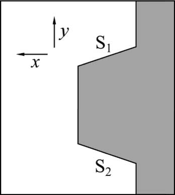
a:	b:
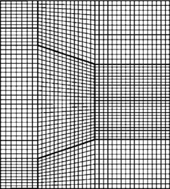
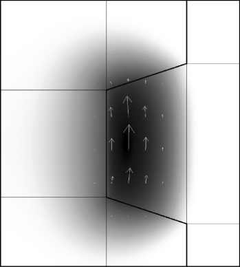
c:	d:

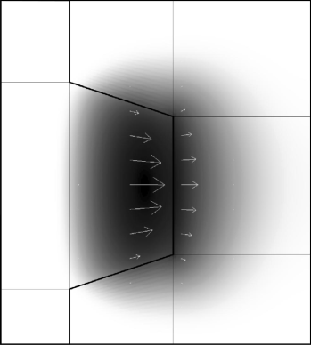
Figure 2: UWA ‘sloping-shoulders’ cryogenic sapphire resonator: (a) medial cross-section through it; the grey(white) shading corresponds to sapphire(vacuum); S₁ and S₂ indicate the sapphire piece’s two (upper and lower) ‘shoulders’. (b) the FEM-based PDE-solver’s meshing of the resonator’s model structure; for clarity only every other meshing line is drawn [i.e. (b) displays the ‘half-mesh’]; (c) magnetic field intensity of the resonator’s WGE_14,0,0 mode; (d) electric field intensity of the same; in both (c) and (d) faint white arrows indicate the direction of the magnetic and electric field, respectively, in the medial plane; ‘intensity’ here means the absolute value of the vectorial H (or, equivalently, B) field, displayed on a logarithmic grey scale –darker being more intense.

The resonator’s form, as the author encoded it into the PDE-solver, is based on figure 3 of ref. [15]. For the simulation presented here, the author took the piece’s outer diameter, the length of its outer axial sidewall, the axial extent of each sloping shoulder, and the radius of each of its two spindles to be, at liquid-helium temperature (i.e. the dimensions here stated include cryogenic shrinkages –see section VI) 49.97, 19.986, 4.996, and 19.988 mm, respectively. The sapphire crystal’s cryogenic permittivities were taken to be $\{\epsilon_{\perp},\epsilon_{\parallel}\}=\{9.2725,11.3486\}$, as stated in ref. [22]. Note that, though coaxial, the sapphire piece and the can do not exactly share a common transverse (‘equatorial’) mirror plane, thus precluding any speeding up of the simulation through the placement (in the model) of a magnetic or an electric wall on the equatorial plane, thereupon halving the 2D region to be analyzed.

Fig. 2(b) displays the FEM-based PDE-solver’s meshing of the resonator structure. Here, the resonator’s interior dielectric domains were regularly decomposed into quadrilaterals (as opposed to triangles), with no quadrilaterals straddling interfaces between different materials. The mesh comprised, in COMSOL’s vernacular, 7296 base-mesh elements and 88587 degrees of freedom (‘DOF’). It typically took around 75 seconds, to obtain the resonator’s lowest (in frequency) 16 modal solutions, for a single, given azimuthal mode order $M$, at [with respect to Fig. 2(b)] full mesh density, on a standard, 2004-vintage personal computer (2.4 GHz, Intel Xeo CPU), without altering the PDE-solver’s default eigensolver settings. With the azimuthal mode order set at $M=14$, the model resonator’s WGE_14,0,0 mode was found to lie at 11.925 GHz, to be compared with 11.932 GHz found experimentally [15].

Wall loss: This mode’s characteristic length $\Lambda$ was determined to be $2.6\times 10^{4}$. Based on ref. [39], one estimates the surface resistance of copper at liquid-helium temperature to be $7\times 10^{-3}\;\Omega$ per square at 11.9 GHz, leading to a wall-loss $Q$ of $3.5\times 10^{11}$ for the WGE_14,0,0 mode. As this is at least an order of magnitude greater than what is observed experimentally, one concludes that wall losses do not substantially limit the UWA resonator’s experimental $Q$.

Filling factor: Using equation 25, the electric filling factors for the WGE_14,0,0 mode have been evaluated. The results, presented in TABLE I, are to be compared with those stated in Table IV of ref. [15]: they are in good agreement with those loc. cit. (labeled ‘FE’), which were obtained via a wholly independent finite-element analysis.

TABLE I: Electric filling factors for the WGE_14,0,0 mode of the UWA resonator

$F_{\rm{diel.}}^{\rm{dir.}}$	radial	azimuthal	axial
sapphire	0.80922	0.16494	$7.016\times 10^{-3}$
vacuum	0.01061	$8.0533\times 10^{-3}$	$1.6543\times 10^{-4}$

V-B Toroidal silica optical resonator [Caltech]

The resonator modeled here, based on ref. [13], comprises a silica toroid, where this toroid is supported through an integral interior ‘web’, such that the toroid is otherwise suspended in free space above the resonator’s substrate. This arrangement is shown in Fig. 3(a). The toroid’s principal and minor diameters are set at $\{D,d\}$ = $\{16,3\}$ $\mu$m, respectively. The silica dielectric is presumed to be wholly isotropic (i.e., no significant residual stress) with a relative permittivity of $\epsilon_{\rm{sil.}}=2.090$, corresponding to a refractive index of $n_{\rm{sil.}}=\sqrt{\epsilon_{\rm{sil.}}}=1.4457$ at the resonator’s operating wavelength (around 852 nm) and temperature. The FEM model’s mesh covered an 8-by-8 $\mu$m square [shown in dashed outlined on the right of Fig. 3(a)] in the medial half-plane containing the silica toroid’s circular cross-section. A pseudo-random triangular mesh was generated (automatically) with an enhanced meshing density over the silica circle and its immediately surrounding free-space; in total, the mesh comprised 5990 (base-mesh) elements, with DOF $=36279$. Temporarily adopting Spillane et al’s terminology, the resonator’s fundamental TE-polarized 93rd-azimuthal-mode-order mode (where by ‘TE’ it is here meant that the polarization of the mode’s electric field is predominantly aligned with the toroid’s principal axis –not transverse to it) was found to have a frequency of $3.532667\times 10^{14}$ Hz, corresponding to a free-space wavelength of $\lambda$ = 848.629 nm (thus close to 852 nm). Using this paper’s equation 24, this mode’s volume was evaluated to be 34.587 $\mu$m³; if, instead, the definition stated in equation 5 of ref. [13] is used, the volume becomes 72.288 $\mu$m³ –i.e. a factor of $n_{\rm{sil.}}^{2}$ greater. These two values straddle (neither agree with) the volume of approx. 55 $\mu$m³, for the same dimensions of silica toroid and the same (TE) mode-polarization, as inferred by eye-and-ruler from figure 4 of ref. [13]. The author cannot explain the discrepancy.

It is pointed out here that the white arrows in Fig. 3 (at least those not anchored on the equatorial plane) are slightly but noticeably oriented away from vertical, indicating that the orientation of the mode’s (vectorial) electric field is not perfectly axial –as per the transverse approximation taken in references [15, 28]. In other words, the arrows’ lack of verticality reveals the inexact- or quasi-ness of the mode’s transverse-electric nature, despite the mode’s relatively high azimuthal mode order ($l\equiv M=93$).

a:

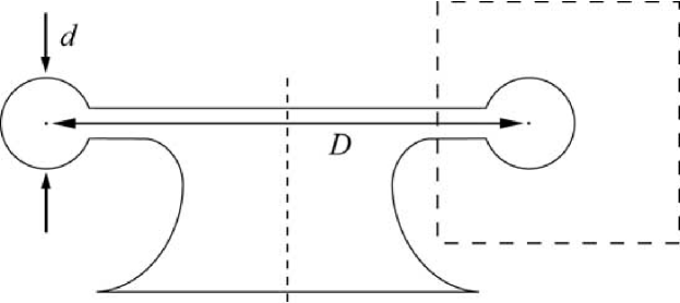
b:

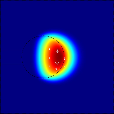
Figure 3: (a) Geometry (medial cross-section) and dimensions of a model toroidal silica microcavity resonator –after ref. [13]; the torus’ principal diameter $D=16$ $\mu$m and its minor diameter $d=3$ $\mu$m; the central vertical dashed line indicates the resonator’s axis of continuous rotational symmetry. (b) False-color surface plot of the (logarithmic) electric-field intensity $|\textbf{E}|^{2}$ within the dashed box appearing in (a) for this resonator’s TE_p=1,m=93 whispering-gallery mode. White arrows indicate the electric field $\bf{E}$’s magnitude and direction in the medial plane.

V-C Conical microdisk optical resonator [Caltech]

The mode volume can be reduced by going to smaller resonators, which, unless the optical wavelength can be commensurately reduced, implies lower azimuthal mode order.

a:

b:

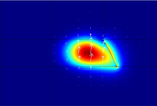
Figure 4: (a) Geometry (medial cross-section) and (half-)meshing of model GaAlAs microdisk resonator –after ref. [14]; the disk’s median diameter is $D$ = 2.12 $\mu$m and its thickness (axial height) $t$ = 255 nm; its conical external sidewall subtends an angle $\theta$ = 26^∘ to the disk’s (vertical) axis; for clarity, only every other line of the true (full) mesh is drawn. The modeled domain in the medial half-plane is a rectangular stretching from 0.02 to 1.5 $\mu$m in the radial direction and from -5 to +5 $\mu$m in the axial direction. (b) False-color surface plot of the (logarithmic) electric-field intensity $|\textbf{E}|^{2}$ for the resonator’s TE_p=1,m=11 mode at $\lambda$ = 1263.6 nm. Again, white arrows indicate the electric field’s magnitude and direction in the medial plane.

The model ‘microdisk’ resonator analyzed here, as depicted in Fig. 4(a) is the author’s attempt at duplicating the structure defined in figure 1(a) of Srinivasan et al [14]; as in their model, the disk’s constituent dielectric (in reality, layers of GaAs and GaAlAs) is approximated as a spatially uniform, isotropic dielectric, with a refractive index equal to $n$ = 3.36. The FEM-modeled domain in the medial half-plane was divided into 4928 quadrilateral base-mesh elements, with DOF $=60003$. Adopting the same authors’ notation, the resonator’s TE_p=1,m=11 whispering-gallery mode, as shown in Fig. 4(b), was found at $2.372517\times 10^{14}$ Hz, equating to $\lambda$ = 1263.6 nm; for comparison, Srinivasan et al found an equivalent mode at 1265.41 nm [as depicted in their figure 1(b)]. The white arrows’ lack of verticality in this article’s Fig. 4(b) implies that the orientation (i.e. polarization) of the magnetic field associated with the true, quasi-TE_p=1,m=11 mode deviates significantly from axial (as would be the case within a transverse approximation).

Mode volume: Using this paper’s equation 24, but with the mode excited as a standing-wave (doubling the numerator while quadrupling the denominator), the mode volume is determined to be $0.1484\times\mu$m${}^{3}\simeq 2.79(\lambda/n)^{3}$, still in good agreement with Srinivasan et al’s $\sim\!2.8(\lambda/n)^{3}$.

Radiation loss: The TE_p=1,m=11 mode’s radiation loss was estimated by implementing both the upper- and lower-bounding estimators described in subsection IV-B. Here, the microdisk and its mode were modeled within a near-spherical volume (equating to a half-disk in the medial half-plane, with a semicircle for its outer perimeter), on whose outer boundary different electromagnetic conditions were imposed –see Fig. 5.

a:

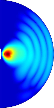
b:

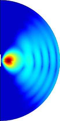
c:

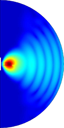
Figure 5: Radiation associated with the same [TE_p=1,m=11, $\lambda$ = 1263.6 nm] whispering-gallery mode as presented in Fig. 4; here, false-color maps of the squared magnitude of the mode’s magnetic field strength are plotted out to the modeled domain’s near-spherical outer boundary, corresponding in the medial half-plane to a semi-circle 12 $\mu$m in diameter, whose center lies at a radial coordinate of 0.01 $\mu$m on the microdisk’s mid-plane. [In reality, the microdisk’s substrate would occupy a considerable part of the meshed half-disk’s lower quadrant, but the model here assumes that, with the exception of the microdisk itself (a dielectric), both quadrants are filled with free space –into which the the whispering gallery mode radiates.] All three maps use the same absolute false-color scale. (a) standing-wave (equal outward- and inward-going) radiation with the outer semicircular boundary set as a magnetic wall; (b) the same but now with the boundary set as an electric-wall; (c) somewhat traveling (more outward- than inward-going) radiation with the boundary’s impedance set to that of an outward-going plane-wave in free space (and with the normal magnetic field constrained to vanish). That (c)’s radiation field is somewhat dimmer than (b)’s is consistent with the different estimates of the resonator’s radiative $Q$ corresponding to (a)-(c) [see text].

With an electric-wall condition (i.e. equations 2 and 3 or, equivalently, 17 and {18, 20}) imposed on the volume’s whole boundary [as per Fig. 5(b)], the right-hand of equation 28 was evaluated. And, with the $\textbf{E}\boldsymbol{\times}\textbf{n}=0$ condition (viz. equation 3) on its outer semi-circle replaced by the outward-going-plane-wave(-in-free-space) impedance-matching condition (viz. equation 30), while the $\textbf{H}\cdot\textbf{n}=0$ condition (equation 2) is maintained, the right-hand side of equation 32 was evaluated for the radiation pattern displayed in Fig. 5(c). For a pseudo-random triangulation mesh comprising 4104 elements, with a DOF of 24927, the PDE solver took, on the author’s office computer, 6.55 and 13.05 seconds, corresponding to Figs. 5(b) and (c), respectively, to calculate 10 eigenmodes around $2.373\times 10^{14}$ Hz, of which the TE_p=1,m=11 mode was one. Together, the resultant estimate on the TE_p=1,m=11 mode’s radiative-loss quality factor is $(1.31<Q_{\rm{rad.}}<3.82)\times 10^{7}$, to be compared with the estimate of $9.8\times 10^{6}$ (at 1265 nm) reported in table 1 of ref. [14]. The standing-wave radiation field in Fig. 5(b) could have been made dimmer (thus increasing $\Lambda$, hence the inferred $Q$) by adjusting (‘tuning’) the meshed half-disk’s diameter –so as to put the microdisk/near-field TE_p=1,m=11 mode, viewed as a secondary source of radiation, closer to an antinode of the cavity’s standing-wave field. Also, the simulations associated with Fig. 5 could certainly have run (with tolerable execution times) on a denser finite-element mesh.

V-D 3rd-order Bragg-cavity alumina:air microwave resonator

Commercial FEM-based PDE-solvers (viz. the COMSOL/FEMLAB package used by the author for this article) permit the simulation of arbitrarily complex structures and, moreover, provide efficient languages and tools for representing and constructing (and modifying) them.

a:

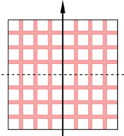
b:

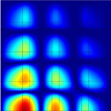
c:

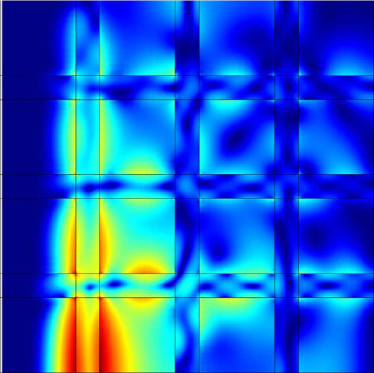
Figure 6: (a) Geometry (medial cross-section) of a alumina:air 3rd-order Bragg-cavity resonator within a cylindrical metallic can (electric walls); the can’s interior surfaces are represented by a solid black line; its interior diameter equals its interior height (and thus this black line takes the form of a square); the horizontal and vertical grey (or pink –in color reproduction) stripes denote cylindrical plates and barrels, respectively, of alumina; white squares correspond to regions of free-space (either air or vacuum); the vertical arrow indicates the resonator’s axis of rotational symmetry; the dashed horizontal line (cf. M1 in Fig. 1) denotes a plane of mirror symmetry, on which an electric or magnetic wall is imposed. (b) False-color plot of the (logarithmic) electric-field intensity $|\textbf{E}|^{2}$ for a zeroth-azimuthal-mode-order ($M=0$) mode at 8.0873 GHz, localized towards the resonator’s center (bottom left in figure); (b) the same but for a sixth-azimuthal-mode-order ($M=6$) mode at 20.0267 GHz, strongly localized in the radial directions but less so in the vertical direction.

Through such a PDE-solver, the method described in sections II through IV can be applied to axisymmetric dielectric resonators of arbitrarily complex medial cross-section, the only requirements being that each such cross-section is (i) bounded (either externally by an enclosure or internally as an excluded region, or both) by metallic walls and (ii) decomposable into definable regions of uniform dielectric. This ability to cope with structural complexity is exemplified here in a modest way through the simulation of a 3rd-order Bragg-cavity alumina:air microwave resonator whose geometry is shown in Fig. 6(a). This resonator’s model geometry was generated straightforwardly through a script written in MATLAB. The resultant FEM mesh in COMSOL comprised 4356 base-mesh elements, with 53067 degrees of freedom (DOF), corresponding to 12 edge vertices per $\lambda/4$ interval of air [i.e., across each white square in Fig. 6(a)], and 6 vertices per $\lambda/4$ interval of alumina [i.e., across each grey/pink ‘strip’, ibid.]. Figs.  6(b) and (c) display two different calculated modes that this resonator supports.

VI Determination of the permittivities of cryogenic sapphire

The author harnessed the method of simulation constructed in sections II and III to extract an independent determination of the two dielectric constants of pure (HEMEX [46]) monocrystalline sapphire at liquid-helium temperature, based on some existing experimental data [47].

a:

b:

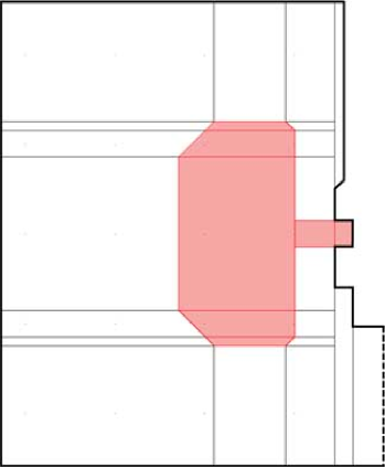
c:

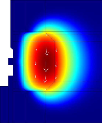
Figure 7: (a) Close-up of one of NPL’s two (nominally identical) Cs-fountain cryo-sapphire resonators, with its outer copper can removed. The resonator’s chamfered HEMEX sapphire ring has an outer diameter of $\sim$46.0 mm and a axial height of $\sim$25.1 mm. This ring’s integral interior ‘web’, 3mm thick, is oriented parallel to and centered (axially) on the ring’s equatorial plane; the web is supported through a central copper post, which is in turn connected [indirectly –through a thin, annular stainless steel ‘shim’ (not visible)] to the resonator’s copper lid (onto which the removed can is secured). Note that the sapphire’s high refractive index falsely exaggerates [cf. the true relative dimensions shown in (b)] the ring’s internal diameter of $\sim$20.0 mm. Above the ring lie two loop probes for coupling, electromagnetically, to the resonator’s operational whispering-gallery mode. [As finally configured, these probes were withdrawn upwards several mm’s closer to the lid and thus further (axially) from the ring]. (b) geometry of the resonator in medial cross-section; pink/grey indicates sapphire, white free space; bounding these dielectric domains, and shown as thick solids lines, are copper surfaces belonging to the resonator’s can, lid and ring-supporting post; the resonator’s cylindrical axis ($r$ or $x=0$) is shown as a dashed vertical line. (c) false-color map (logarithmic scale) of the magnetic (H) field’s squared magnitude for the resonator’s 11th-azimuthal-mode-order fundamental quasi-transverse-magnetic (N1₁₁ in ref. [45]’s notation) whispering-gallery mode at 9.146177 GHz (simulated), as detailed on the 6th row of TABLE II. The white arrows indicate the magnitude and direction of this mode’s electric (E) field in the medial plane.

This data, as is listed in the four right-most columns of TABLE II, comprised: the centre frequencies, FWHM widths, turnover temperatures, and ‘Kramers’ splittings for a set of 16 resonances, as measured on a (one of a pair of) cryogenic sapphire resonator(s), as shown, without its enclosing can, in Fig. 7(a). Only two resonances out of this set (viz. N1₁₁ and S2₉) had hitherto been identified –via MAFIA [7, 9] simulations.

TABLE II: NPL’s cryogenic sapphire resonator: simulated and experimental WG modes compared

Simulated	Simul.	Simul.	Mode	Experi-	Exper.	Exper.	Exper.
minus	perp.	para.	ID	mental	width	turn-	Kram.
experim.	filing	filling		freq.		over	split.
frequency	factor	factor				temp.
$[$MHz$]$				$[$GHz$]$	$[$Hz$]$	$[$K$]$	$[$Hz$]$
-0.451	0.860	0.090	S26	6.954664	285		780
-0.945	0.930	0.028	S27	7.696176	82.5	$<4.2$	158
0.881	0.453	0.517	S46	8.430800
-1.538	0.951	0.014	S28	8.449908	44.5	$<4.2$	418
-0.412	0.674	0.299	N28	9.037458		$4.8$
-2.208	0.071	0.917	N111	9.148385	9	$5.0$	57
-1.916	0.960	0.009	S29	9.204722	15.5	$<4.2$	88
0.498	0.251	0.733	S110	9.267650	12	$5.2$	180
1.055	0.287	0.685	N48	9.421207	80	$5.0$
-0.177	0.437	0.543	S38	9.800335	84	$4.8$	1850
0.358	0.223	0.763	S111	9.901866	10	$5.0$	160
-2.269	0.965	0.007	S210	9.957880	24	$<4.2$
1.32	0.730	0.246	S48	10.27242	153	$5.0$
0.19	0.200	0.787	S112	10.53863	9.5	$4.9$	24
0.00	0.181	0.808	S113	11.17728	24.5	$4.9$	42
4.13	0.972	0.006	S212	11.44918	10	$5.2$

This cryo-sapphire resonator’s complete, detailed model geometry, as shown in Fig. 7(b), was coded into a MATLAB script. This script contained, for example, the dimensional parameters specifying the form of the sapphire ring’s (large) external and (smaller) internal chamfers. The model geometry took into account the shrinkages of the resonator’s constituent materials from room temperature (293 K) down to liquid-helium temperature (4.2 K). The two cryo-shrinkages of sapphire (a uniaxial crystal) were calculated by integrating up [48] the linear-thermal-expansion data stated in Table 4 of ref. [49] (identical to that stated in TABLE 1 of ref. [50]): $(1.0-7.21\times 10^{-4})$ and $(1.0-5.99\times 10^{-4})$ for directions parallel and perpendicular to sapphire’s c-axis, respectively. The cryo-shrinkage of (isotropic) copper was taken directly from Table F at the back of ref. [51]: $(1.0-3.26\times 10^{-3})$. The values of sapphire’s two dielectric constants were initially set equal to those specified in ref. [22]: $\epsilon_{\perp}=9.2725$ and $\epsilon_{\parallel}=11.3486$.

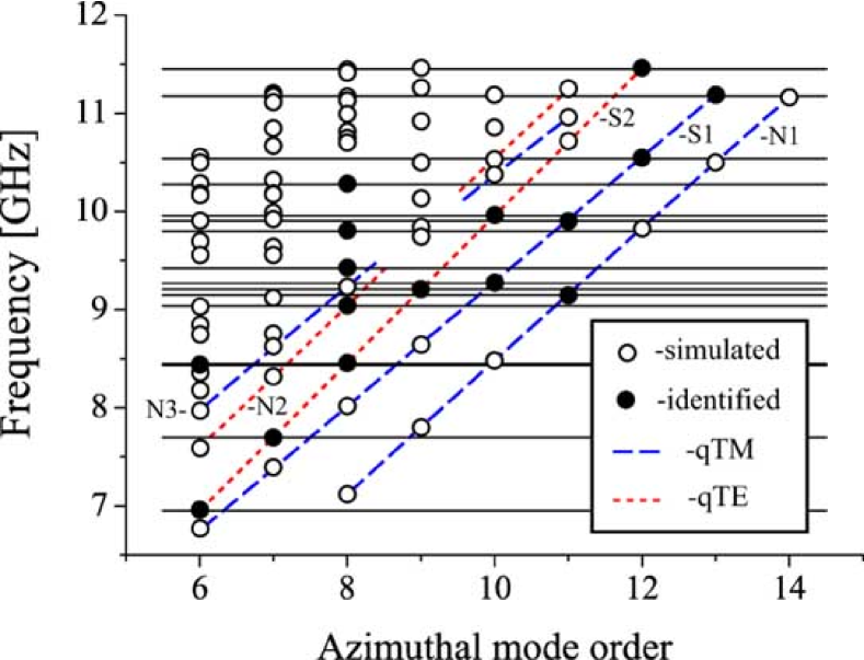
Figure 8: Plot used to identify experimentally measured with simulated WG modes. Solid horizontal lines (16 in total) indicate the center frequencies of the former. Solid circles indicate the identification of a simulated mode with an experimental one (the difference in their frequencies corresponds to much less than a circle’s radius in all cases); hollow circles indicate simulated modes that were not identified with any experimentally measured one. Quasi-transverse-magnetic (q-TM) and quasi-transverse-electric (q-TE) WG modes of the same family are joined by (blue-)dashed and (red-)dotted lines respectively; a few of the lowest-lying mode families are labeled using standard notation [45].

Fig. 7(b)’s geometry was meshed with quadrilaterals over the medial half-plane, with 8944 elements in its base mesh, and with DOF $=108555$. [These quadrilaterals followed the sloping chamfers of the resonator by taking the shape of trapezoids.] For a given azimuthal mode order $M$, the calculation of the lowest 16 eigenmodes took around 3 minutes on the author’s office PC (as previously specified). Fig. 7(c) shows the form of the resonator’s N1₁₁ whispering-gallery mode, corresponding to the 6th row of TABLE II. Filling factors were then calculated to quantify each frequency’s sensitivity to changes in the sapphire’s two dielectric constants ($\epsilon_{\parallel}$ and $\epsilon_{\perp}$). The author identified each of the 16 experimental resonances with a particular simulated WG mode, aiming to minimize the residual (simulated-minus-measured) frequency difference (i.e. the sum $\chi^{2}$ variance over the left-most column in TABLE II), whilst requiring that the other measured attributes (e.g. insertion loss, linewidth) of the resonances identified to the same ‘family’ of WG modes (e.g. S1 or N2) varied smoothly with the azimuthal mode order $M$. With the identifications of the experimental modes ‘locked’ as per the 4th column of TABLE II, the model’s two sapphire dielectric constants were adjusted from their initial values to minimize $\chi^{2}$ (‘least squares’). The resultant best-fit values were:

$$\epsilon_{\perp} = 9.285\,\,(\pm 0.010);$$ (33)

$$\epsilon_{\parallel} = 11.366\,\,(\pm 0.010).$$ (34)

With the two dielectric constants set to these values, the WG modes were recalculated (an in-principle superfluous check); the first three columns in TABLE II result from this recalculation (the filling factors hardly changed from their original fitted values). Pending the construction of a more detailed and precise error budget, the provisional $\pm 0.010$ uncertainty assigned to the values of both dielectric constants reflects their observed shifts upon refitting with a few ‘problematic’ experimental modes identified with different simulated ones . Compared to these identification-related shifts, the systematic errors associated with a finite meshing density –as analyzed quantitatively in ref [33]), or the experimental uncertainties associated with the resonator’s geometric shape (particularly the diameter and height of the sapphire ring) were quite negligible. The specified (i.e. contracted) tolerance on the alignment of the sapphire crystal’s c-axis with respect to the geometric axis of the ‘cored’ cylinder from which the two rings were cut (through orientation-preserving methods) was only $<0.5$ degrees. Though the effects of crystal misalignment cannot be modeled quantitatively with the method presented in this paper, for which axial symmetry is a requirement, it can be estimated that, given the $\sim$two-parts-in-ten contrast between the sapphire’s parallel and transverse permittivities, such a misalignment should make a significant/dominant contribution to the  1-part-in-a-thousand residuals between the simulated and measured center frequencies (and thus the determination of $\epsilon_{\perp}$ and $\epsilon_{\parallel}$.) Even with azimuthal mode orders of $M\sim 10$, as is the case here, the narrowness of the measured WG resonances’ Kramers splittings (listed in the right-most column of TABLE II, and generally less than 1 part per million relative to the absolute frequency) would indicate a much higher degree of rotational invariance, however. Though noting that center-frequency residuals of a few parts per thousand are not untypical for FEM-based simulations of WG modes [33], the author has yet to reconcile, convincingly, the residuals with their cause(s) –as would be required to construct a more detailed error budget.

VII Conclusion

This paper demonstrates, through the explicit statement of weak-form expressions and boundary constraints, how a commercial (FEM-based) PDE-solver can be configured to simulate, quickly and to high accuracy, the whispering-gallery modes of axisymmetric dielectric resonators on standard computer hardware. The source codes/configuration scripts used to implement the simulations presented in section V of this paper are freely available from the author.

Mark Oxborrow was born near Salisbury, England, in 1967. He received a B.A. in physics from the University of Oxford in 1988, and a Ph.D. in theoretical condensed-matter physics from Cornell University, Ithaca, NY, in 1993; his thesis topic concerned random-tiling models of quasicrystals. During subsequent postdoctoral appointments at both the Niels Bohr Institute in Copenhagen and back at the University of Oxford, he investigated acoustic analogues of quantum wave-chaos. In 1998, he joined the UK’s National Physical Laboratory; his research there to date has included the design and construction of ultra-frequency-stable microwave and optical oscillators, the development of single-photon sources, and the applications of carbon nanotubes to metrology.

.

Appendix A Configuration of COMSOL Multiphysics for simulating axisymmetric dielectric resonators: explicit weak-form expressions

It is here explained, in some detail, how to set up a dielectric-resonator simulation in COMSOL Multiphysics [10] –from scratch. These explanations should also be helpful to anyone wishing to modify one of the author’s existing models –as incarnated in an .MPH file. At least in the first instance, it is recommended that the following instructions be meticulously adhered to –lest one stray from a tried-and-tested path. And it is suggested that the reader work through them with COMSOL Multiphysics open and running on his/her desktop. All menu items, expression names and variables associated with the program are displayed in typed text font. A good deal of supplementary information can be found in the documentation supplied with COMSOL Multiphysics itself; the author found the following chapters therein to be the most useful/relevant: ‘PDE Modes for Equation-Based Modeling’, ‘The Weak Form’, and ‘COMSOL Multiphysics Scripting’. Upon reading these chapters, one might be left with the impression that COMSOL is simply not sufficiently flexible to embrace the task in hand (i.e. to implement sections II through IV of this article explicitly); the following instructions demonstrate how COMSOL Multiphysics can, despite these first impressions, and most straight-forwardly, be so configured to implement the 2D simulation of isotropic dielectric resonators. From the beginning then:

TABLE III: COMSOL Constants –included in weak-form expressions

Name	Expression	Description [unit]
	(= value)
c	299792458	speed of light (exact) [m/s]
cbar	2*pi/c	frequency constant [s/m]
	( = 2.095845e-8)
cbar2	4*pi^2/c^2	frequency constant [s2/m2]
	( = 4.392566e-16)
alpha	1.0	penalty-term coefficient
M	9	azimuthal mode order
e0	1.0	relative permittivity
		of free-space
e1	n_AlGaAs^2	relative permittivity of
	( = 11.2896)	isotropic_dielectric_1
e2	1.0	same but of
		isotropic dielec._2
e3	1.0	etc.
eperp0	1.0	relative permittivity
		of free-space
		in directions transverse
		to cylindrical axis
epara0	1.0	same but in direction
		parallel to cylindrical axis
eperp1	9.2725	relative permittivity of
		uniaxial_dielectric_1
		in directions transverse
		to cylindrical axis
epara1	11.3486	same but in direction
		parallel to cylindrical axis
epara2	1.0	relative permittivity of
		uniaxial_dielectric_2
		transverse to cyl. axis
eperp2	1.0	same but parallel to
		cylindrical axis
eperp3	1.0	etc.
epara3	1.0	etc.
e_293K_alumina	9.8	relative permittivity of
		alumina at room temperature
epe_4K_sap_UWA	9.2725	UWA values for cryogenic
		HEMEX sapphire
epa_4K_sap_UWA	11.3486
epe_293K_sap	9.407	nominal room temperature
		values for same
epa_293K_sap	11.62
epe_4K_sap_NPL	9.2848	Values fitted to
		NPL Cs-fountain
		HEMEX resonator
epa_4K_sap_NPL	11.3660
n_silica	1.4457	refractive index of
		thermally grown
		silica (Fig B.2, p. 172 of
		ref. [28])
n_AlGaAs	3.36	average refractive index of
		GaAs and AlGaAs layers
		(p. 172 of ref. [14])
mf	2.374616e14	match frequency
ttgH	1	toggle
ttgE	0	toggle
mix_ang	45	electric-magnetic mixing
		angle (in degrees)
cMW	sin(mix_ang
	* pi /180)	magnetic-walled-ness
	(= 0.707107)
cEW	cos(mix_ang
	* pi /180)	electric-walled-ness
	(= 0.707107)
tngM	1
tngE	0

A-A Setting up –fundamentals

Get COMSOL Multiphysics up and running. Access the Model Navigator panel via File $\Rightarrow$ New ... and select the New tab if not already selected.

(a) Select ‘2D’ from the Space dimension: drop-down menu [note: do not choose ‘Axial symmetric (2D)’].

(b) Browse to and select ‘COMSOL Multiphysics $\Rightarrow$ PDE Modes $\Rightarrow$ Weak Form, Subdomain’ from the Application Mode navigator.

(c) Type (verbatim) ‘Hrad Hazi Haxi’ into the Dependent variables: text field. These three variables are the radial, azimuthal and axial components of the magnetic field strength, respectively; all three are dependent on (i.e. are functions of) the Cartesian coordinates for the COMSOL simulation’s 2D space, namely x (horizontal on the screen) and y (vertical) –both in units of metres [m]. The coordinate names ‘x’ and ‘y’ are already fixed by COMSOL (i.e. they are reserved symbols) and need not be explicitly entered (in COMSOL terminology, x and y are ‘geometric variables’).

(d) For the Application mode name: (default u) one can type in anything one likes.

(e) Select ‘Lagrange - Quadratic’ from the Element: drop-down menu. [This choice is proven to work.]

A-B Constants

All of the various constants (i.e. independent of x or y) included within the weak-form expressions given below are defined and described in TABLE III. The equivalent of this table needs to be typed (or loaded) into COMSOL’s Options $\Rightarrow$ Constants .... Each Expression thus Value therein [except those for e0, eperp0, epara0 –which define the (unit) relative permittivity of free-space], can be user-varied. But every Name should be entered verbatim; i.e., each constant must be named exactly as it appears in the expressions that subsequently include it.

A-C Expressions (for Postprocessing)

The post-processing of the calculated magnetic-field strength (as a function of position) for each solved eigenfunction is facilitated through the various definitions presented here.

A-C1 Scalar expressions

The equivalent of TABLE IV (or some subset thereof) needs to be typed into COMSOL’s Options $\Rightarrow$ Expression ... $\Rightarrow$ Scalar expressions ....

TABLE IV: COMSOL Scalar Expressions –for postprocessing

Name	Expression
	(Description)
DivH	(Hrad-Hazi*M+(Haxiy+Hradx)*x)/x
	(divergence of magnetic field –should be zero!)
MagEnDens	Hrad*Hrad+Hazi*Hazi+Haxi*Haxi
	(magnetic energy density)
Drad	(Haxi*M-Haziy*x)/x
	(radial component of electric displacement)
Dazi	-Haxix+Hrady
	(azimuthal component of electric displacement)
Daxi	(Hazi-Hrad*M+Hazix*x)/x
	(axial component of electric displacement)
Erad	Drad/eperp
	(radial component of electric field strength)
Eazi	Dazi/eperp
	(azimuthal component of electric field strength)
Eaxi	Daxi/epara
	(axial component of electric field strength)
ElecMagSqrd	Erad*Erad+Eazi*Eazi+Eaxi*Eaxi
	(electric field strength magnitude squared)
ElecEnDens	Erad*Drad+Eazi*Dazi+Eaxi*Daxi
	(electric energy density)
AbsMagEnDens	abs(Hrad)^2+abs(Hazi)^2
	+abs(Haxi)^2
	(absolute magnitude energy density)
MagNrmlHSqrd	2*pi*x*abs(Haxi*ny
	+Hrad*nx)^2
	(magnitude normal mag. field strength squared)
MagTngHSqrd	2*pi*x*(1*abs(Hazi)^2
	+1*abs(Haxi*nx-Hrad*ny)^2)
	(magnitude tangential magnetic field squared)
AbsElecSqrd	abs(Erad)^2+abs(Eazi)^2
	+abs(Eaxi)^2
	(absolute electric field squared)

A-C2 Subdomain expressions

The functionality of Subdomain expressions is required for generating post-processed fields, like the electric field strength E –as per the 6th, 7th and 8th entries in TABLE IV. Those constants associated with each such field’s definitions, like (in the case of E) the relative permittivities epara and eperp, vary from one subdomain within the medial half place to another. The variation of these subdomain-dependent ‘constants’ is represented through Options $\Rightarrow$ Expressions $\Rightarrow$ Subdomain expressions; therein, the Name of each such variable is the same in each and every Subdomain (as identified by an integer), but its Expression reflects the variable value in the selected Subdomain. Thus, the Expression for epara in a Subdomain corresponding to (cryogenic and axisymmetrically oriented) sapphire would be epara1, with epara1 defined (globally) as 11.3486 (or whatever) through TABLE III, whereas in a Subdomain corresponding to free space, the Expression for epara should be set to 1. Similarly (and more simply), the single Subdomain-dependent variable erel can be used to represent the variation of relative permittivity within an axisymmetric resonator containing solely isotropic dielectrics (incl. free space).

A-D Weak-form expressions

The simulation’s defining weak-form expressions are set up through the Physics $\Rightarrow$ Subdomain Settings ... control panel. On the left of this panel, first select the Groups tab. A New Group must be named and defined for each dielectric within the resonator being simulated. The author chose to name these dielectric Groups ‘dielectric_0:vacuum’, ‘dielectric_1’, …, ‘dielectric_n’, … . For each dielectric Group, (in general) dielectric_n say, corresponding weak-form expressions need to be entered into the weak terms (i.e. three slots or text fields), for expressions involving spatial derivatives, and also into the dweak terms, for expressions involving temporal derivatives; these slots are accessed through the weak and dweak tabs, respectively, located on the right of the Subdomain Settings ... control panel. These terms govern the electromagnetic field in regions filled with the $n$-th dielectric, as specified in the Constants ... table introduced above. No other fields on the right of Subdomain Settings ... need(/should) be touched; in particularly, don’t monkey with the contr-tabbed sub-panel. Note that it is imperative that the Name of each constant entered into Options $\Rightarrow$ Constants ... above match (verbatim) its appearances within the expressions (below) that are entered into the weak and dweak text fields here. For each dielectric Group, two weak and one dweak terms are required: (i) a ‘Laplacian’ term (corresponding to the left most term on the left-hand side of equation 1 and (ii) a ‘penalty’ term, included to suppress spurious modes, corresponding to the middle term of the same.

A-D1 Laplacian term [first weak-term slot]

: The form of the Laplacian weak term, $(\boldsymbol{\nabla}\boldsymbol{\times}\tilde{\textbf{H}}^{*})\frac{\cdot}{\boldsymbol{\epsilon}}\;(\boldsymbol{\nabla}\boldsymbol{\times}\textbf{H})$, here given for the 1st axisymmetric dielectric, is

((eperp1*(test(Hazi)*Hazi

-M*(test(Hazi)*Hrad

+Hazi*test(Hrad))

+M^2*test(Hrad)*Hrad)

+epara1*M^2*test(Haxi)*Haxi)/x

+eperp1*(test(Hazix)*(Hazi-M*Hrad)

+Hazix*(test(Hazi)-M*test(Hrad)))

-epara1*M*(test(Haxi)*Haziy

+Haxi*test(Haziy))

+x*(eperp1*test(Hazix)*Hazix

+epara1*((test(Haxix)

-test(Hrady))*(Haxix-Hrady)

+Haziy*test(Haziy)))

)/(epara1*eperp1)

(35)

where Hazix denotes the partial derivative of Hazix with respect to the coordinate x, Hrady the partial derivative of Hazi with respect to y, etc.; test(Hazi) denotes the ‘test function’ of Hazi, etc. Its equivalent for the 2nd axisymetric dielectric is obtained by replacing eperp1 by eperp2 and epara1 by epara2, and so forth for all other axisymetric dielectrics (should more be required). The above expression can be significantly simplified for the (subdomain) Groups corresponding to isotropic dielectrics or free space (viz. dielectric_0); for computational efficiency, it is recommended that these simplifications be implemented wherever possible. The required form of the Laplacian weak term, $[(\boldsymbol{\nabla}\boldsymbol{\times}\tilde{\textbf{H}}^{*})\cdot(\boldsymbol{\nabla}\boldsymbol{\times}\textbf{H})]/{\epsilon_{1}}$, for the 1st isotropic dielectric is given explicitly as

((test(Hazi)*Hazi

-M*(test(Hazi)*Hrad

+Hazi*test(Hrad))

+M^2*(test(Hrad)*Hrad

+test(Haxi)*Haxi))/x

+(test(Hazix)*(Hazi-M*Hrad)

+Hazix*(test(Hazi)-M*test(Hrad)))

-M*(test(Haxi)*Haziy

+Haxi*test(Haziy))

+x*(test(Hazix)*Hazix

+((test(Haxix)

-test(Hrady))*(Haxix-Hrady)

+Haziy*test(Haziy))))/e1 ,

(36)

where e1 is the material’s dielectric constant (as appearing in TABLE III). The Laplacian weak term for the vacuum is the same with $\epsilon_{1}\rightarrow 1$, and those for other isotropic dielectrics are similarly obtained by swopping $\epsilon_{1}$ with $\epsilon_{2}$, $\epsilon_{3}$, and so forth.

A-D2 Penalty (divergence-suppressing) term [second weak-term slot]

: The form of the penalty weak term, $\alpha(\boldsymbol{\nabla}\cdot\tilde{\textbf{H}}^{*})\cdot(\boldsymbol{\nabla}\cdot\textbf{H})$, the same for each subdomain Group, is

alpha*((test(Hrad)*Hrad

-M*(test(Hazi)*Hrad

+Hazi*test(Hrad))

+M^2*test(Hazi)*Hazi)/x

+(test(Haxiy)

+test(Hradx))*(Hrad-M*Hazi)

+(test(Hrad)-M*test(Hazi))

*(Hradx+Haxiy)

+x*(test(Hradx)

+test(Haxiy))*(Hradx+Haxiy))

(37)

here, the coefficient alpha (whose value is determined through COMSOL’s equivalent of TABLE III) controls the aggressiveness of the divergence suppression induced by this term. The remaining, 3rd slot, should be zero-filled. [As a general rule, unused weak-form slots should always be filled with zeroes –this applies to the the dweak term slots below.]

A-D3 Frequency term [first dweak-term slot]

The form of the temporal-derivative/frequency (so-called ‘dweak’) term $\tilde{\textbf{H}}^{*}\cdot\partial^{2}\textbf{H}/{\partial^{2}t}$, common to all subdomain Groups, is entered into the first slot within the dweak-tabbed panel of Physics $\Rightarrow$ Subdomain Settings ..., and is given as

cbar2*x*(Haxitt*test(Haxi)

+Hazitt*test(Hazi)

+Hradtt*test(Hrad)),

(38)

where Haxitt denotes the double partial derivative of Haxi with respect to time, etc. The remaining 2nd and 3rd slots of the dweak-tabbed panel should be zero-filled.

A-E Boundary conditions

Here the constraints stated in subsection II-C are expressed in COMSOL-ready forms. The model resonator’s boundary conditions are defined through the Physics $\Rightarrow$ Boundary Settings ... control panel. On the left of this panel, select the Groups tab. Each named boundary Group here corresponds to a particular electromagnetic boundary condition, the most essential of which are described here. These different e.m. boundary conditions are specified by the expressions that populate the three slots within their respective contr-tabbed sub-panels, located on the right-hand side of Boundary Settings ...; ‘contr’ here stands for ‘constraint’. [The neighboring weak-tabbed and dweak-tabbed panels within the Boundary Settings ... need not be touched (and left zero-filled).]

A-E1 Electric wall (for a bounded isotropic dielectric)

Hrad*nx+Haxi*ny;

(39)

-Haxix+Hrady;

(40)

(Hazi*nx-Hrad*M*nx

-Haxi*M*ny+Hazix*nx*x

       +Haziy*ny*x)/x;

(41)

here nx and ny are, as ‘geometric variables’ within COMSOL (in 2D), the components of the (outward) unit normal vector on the boundary of a subdomain.

A-E2 Magnetic wall (for a bounded isotropic dielectric)

Haxi*nx-Hrad*ny;

(42)

Hazi;

(43)

(Haxi*M*nx+Hazi*ny

-Hrad*M*ny-Haziy*nx*x

       +Hazix*ny*x)/x.

(44)

A-E3 Radiation match (in free-space)

As has already been discussed in subsection II-C, the constraints appropriate to implementing a radiation match, can be regarded (complex) linear combinations or ‘mixings’ of pure electric- and magnetic- wall constraints. The first constraint mixes the magnetic-wall constraint 23, i.e. 43 above, with the electric-wall constraint 20, i.e. 41 above:

-i*cMW*Hazi*cbar*mf

+cEW*(Hazi*nx-Hrad*M*nx

-Haxi*M*ny+Hazix*nx*x

+Haziy*ny*x)/x;

(45)

note that ‘i’ here is the square root of minus one. And the second constraint mixes the electric-wall constraint 18, i.e. 40 above, with the magnetic-wall constraint 22, i.e. 42 above:

-i*cEW*(-Haxix+Hrady)

+cMW*cbar*mf*(Haxi*nx-Hrad*ny).

(46)

Here, the pair of constants {cMW and cEW}, are defined through TABLE III. When they are set to their standard (default) values of { $1/\sqrt{2}$, $1/\sqrt{2}$ }, equations 45 and 46 impose a radiation match on tangential field components at the impedance of plane e.m. waves in free-space. Here also, cbar$=\bar{c}\equiv 2\pi/c$; and mf is the mode’s (center) frequency; both need to be defined within Options $\Rightarrow$ Constants .... –as per their corresponding rows in TABLE III;

The final (optional) constraint mixes the electric wall constraint 17, i.e. 42 with the magnetic wall constraint 21, i.e. 44:

tngM*cbar*mf*(Hrad*nx+Haxi*ny)

-tngE*(Haxi*M*nx+Hazi*ny

-Hrad*M*ny-Haziy*nx*x

+Hazix*ny*x)/x.

(47)

Here; the constants tngM and tngE, are also defined through TABLE III and thereupon Options $\Rightarrow$ Constants .... Setting {tngM, tngE} = {1,0}({1,0}) constrains the magnetic (electric) field to be wholly tangential on the impedance-matching plane as is characteristic of electromagnetic traveling waves. The default setting for this third constraint was (arbitrarily) {tngM, tngE} = {1,0}). [It is remarked here that the author sought to implement the radiation-matching constraints more directly and elegantly with time derivatives, i.e., replacing 2*pi*mf*Hazi by Hazit, and similarly for Hrad and Haxi. But COMSOL did not generate the intended frequency factor when interpreting them. He thus resorted to entering the expressions as stated in equations 45 through 47, requiring mf to be set, by hand, for each mode.]

A-F Geometry

Each resonator’s geometry needs to be either constructed within or imported into COMSOL. COMSOL’s manual provides instructions on how to implement both. Though simple geometries (e.g. a cylinder of solid dielectric material inside a cylindrical metal can) can be quickly constructed by hand within COMSOL, the author found it advantageous to define the sets of quadrilateral subdomains into which many axisymmetric dielectric resonators can be readily decomposed using MATLAB scripts, where the script was run to generate the resonator’s medial cross-section. The key lines in these scripts were those of the form

q1 = poly2vert([[x1,y1];
[x2,y2];[x3,y3];[x4,y4]]);

this particular line defines a quadrilateral, named q1, whose vertices have the x-y coordinates: [x1,y1], ... [x4,y4]. These quadrilaterals could then be imported into COMSOL by entering a list comprising their names into File $\Rightarrow$ Import $\Rightarrow$ Geometry Objects. Each complete MATLAB script (also available from the author upon request) included, where known/relevant, the cryogenic shrinkages of the resonator’s constituent materials.

A-G Meshing

If constructed out of quadrilaterals, the resonator’s geometry can be meshed either into sub-quadrilaterals using Mesh $\Rightarrow$ Map Mesh. Else, the geometry can always be meshed into (psuedo-random) triangles using Mesh $\Rightarrow$ Initial Mesh with (recommended) mesh refinement over selected areas (covering the bright spots of WG modes). Note that, for the geometry to be Map Mesh-able, the vertices of its internal quadrilaterals should generally all meet at ‘cross-roads’, where, at each, four vertices belonging to four separate quadrilaterals all meet at a point, as opposed to ‘T-junctions’, where, at each, two vertices belonging to two separate quadrilaterals meet at a point along the boundary edge of a third quadrilateral. The reader is advised to consult the COMSOL manual (chapter ‘Meshing’, section ‘Generating Meshes’, subsection ‘Creating Mapped Meshes in 2D’) for a fuller (though a still not wholly satisfactory) explanation of this rather quirky requirement. The meshing density can be controlled by, for selected edges, activating and entering an appropriate integer in the ‘Contrained edge element distribution’ field within of the Boundary tab of the Map Mesh control panel. With regard to both Map Mesh-ability and control over meshing density, it can be advantageous (or plain necessary) to divide odd-shaped subdomains (e.g. an ‘L’-shaped region covered throughout by a single spatially uniform dielectric material) into several, more simply shaped adjoining subdomains (e.g., in the case of dividing up the L-shaped subdomain, two or even three rectangular subdomains). Note that the geometry will not mesh if the allocations of elements along too many edges are (inconsistently) specified; in other words, the edge element distribution must not be over constrained.

A-H Assignments

A-H1 Interiors of subdomains

The (either hand-made or imported) quadrilaterals composing the resonator’s cross-sectional geometry are assigned to one of the defined dielectric Groups via the Subdomain Settings ... $\Rightarrow$ Subdomains tab. Activating (i.e. ticking) the Select by group option here aids the verification of assignments.

A-H2 Edges of subdomains

The external edges of quadrilaterals should be set be obey one of the three above-described Group boundary conditions via the Physics $\Rightarrow$ Subdomain Settings ... $\Rightarrow$ Subdomains tab. COMSOL appears to be smart enough to recognize those edges that are external on its own accord and automatically ‘ghosts’ (grays) internal edges; the latter should not be assigned to any boundary Group condition. Thus, with the Select by group feature activated, all the appropriate edges can be assigned to the appropriate (usually electric-wall) boundary condition in a single selection of the Groups drop-down menu.

A-I Solution

In Solve $\Rightarrow$ Solve Parameters:

(a) set the selected Solver: to ‘Eigenvalue:’;

and, with the General tab selected,

(b) set the Desired number of eigenvalues: to ‘10’ –or whatever ones desires;

(c) set Search for eigenvalue around: to ‘0’ –or whatever;

(d) set Linear system solver: to ‘Direct (SPOOLES) (this is at least the author’s starting recommendation);

(e) set Matrix symmetry: to Symmetric’.

Having implemented all of the above, one should now be able to Solve $\Rightarrow$ Solve Problem.

A-J Postprocessing

COMSOL Multiphysics’ standard documentation explains how to configure and use of the Postprocessing $\Rightarrow$ Plot Parameters control panel. Only a few specific pointers are supplied here:

[1] The center frequencies of solved resonances can be viewed through the Solution to use $\Rightarrow$ Eigenvalue: drop-down menu in the General-tabbed sub-panel of the Plot Parameters control panel.

[2] To display the morphology and features of the solved eigenmodes, the Expression: slot within the Surface-tabbed sub-panel of the same is filled with either (i) some function of the solved field variables {Hrad, Hazi, Haxi } or (ii) one of those expressions (e.g. ElecMagSqrd) pre-defined in Options $\Rightarrow$ Expressions Scalar Expressions as COMSOL’s equivalent of TABLE IV, or (iii) some function/combination thereof. For example,

log10(AbsMagEnDens+10^(-10))

(48)

can be inserted to view the magnetic energy density on a logarithmic scale. To view (as a diagnostic) the divergence of the magnetic field strength, which should be zero, one inserts DivH $\equiv$ (Hrad-Hazi*M+(Haxiy+Hradx)*x)/x instead.

[3] Determinations of an electromagnetic mode’s volume, filling factor(s), and length ($\Lambda$), as per equations 24, 25, and 27, respectively, all make use of the Postprocessing $\Rightarrow$ Domain Integration panel. For example, the numerator $\int\int\int_{\rm{h.-s.}}\epsilon|\textbf{E}|^{2}\textrm{d}\textrm{V}$ on the right-hand-side of 24 can be evaluated by inserting ElecEnDens $\equiv$ Erad*Drad+Eazi*Dazi+Eaxi*Daxi into this panel’s Expression: slot, with those entries selected in the Subdomain selection list on the left-hand side of the same panel covering all significant parts of the mode’s bright spot.

[4] With regards to determining filling factors, the numerator on the right-hand side of equation 25 can be evaluated by selecting only those subdomains filled with the relevant dielectric (as opposed to free-space).

[5] To determine the resistive-wall-loss integral $\int|\textbf{n}\boldsymbol{\times}\textbf{H}|^{2}\textrm{d}\textrm{S}$ (forming the denominator of equation 27), one uses the Postprocessing $\Rightarrow$ Boundary Integration panel with 2*pi*x*(abs(Hazi)^2 +abs((Haxi*nx -Hrad*ny))^2) inserted into the Expression: slot within the Expression to integrate box therein, and where entries selected with Boundary selection correspond to the resonator’s enclosing (metallic and lossy) surfaces.

[6] The maximum/minimum of a field variable, as required to evaluate the denominator on the right-hand side of 24, can be determined through the Postprocessing $\Rightarrow$ Plot parameters $\Rightarrow$ Max/Min, wherein the Expression: slot is filled with the field variable’s expression (viz. ElecEnDens for evaluating said denominator).

References

- [1] K. S. Kunz, The finite difference time domain method for electromagnetics. CRC Press, 1993.
- [2] S. V. Boriskina, T. M. Benson, P. Sewell, and A. I. Nosich, “Highly efficient design of specially engineered whispering-gallery-mode laser resonators,” Optical and Quantum Electronics, vol. 35, pp. 545–559, mar/apr 2003, see http://www.nottingham.ac.uk/ggiemr/Project/boriskina2.htm.
- [3] J. Ctyroky, L. Prkna, and M. Hubalek, “Rigorous vectorial modelling of microresonators,” in Proc. 2004 6th International Conference on Transparent Optical Networks, 4-8 July 2004, vol. 2, 2004, pp. 281–286.
- [4] O. C. Zienkiewicz and R. L. Taylor, The finite element method, 5th ed. Butterworth Heinemann, 2000, vol. 1: ‘The Basis’.
- [5] J. U. Nöckel and A. D. Stone, “Ray and wave chaos in asymmetric resonator optical cavities,” Nature, vol. 385, pp. 45–47, 1997.
- [6] M. Sumetsky, “Whispering-gallery-bottle microcavities: the three-dimensional etalon,” Opt. Lett., vol. 29, pp. 8–10, 2004.
- [7] “MAFIA,” CST GmbH, Bad Nauheimer Str. 19, D-64289 Darmstadt Germany. [Online]. Available: http://www.cst.de/Content/Products/MAFIA/Overview.aspx
- [8] R. Basu, T. Schnipper, and J. Mygind, “10 GHz oscillator with ultra low phase noise,” in Proc. The Jubilee 8th International Workshop ‘From Andreev Reflection to the International Space Station’, Björkliden, Kiruna, Sweden, March 20-27, 2004, 2004. [Online]. Available: http://fy.chalmers.se/ f4agro/BJ2004/FILES/Bjorkliden_art.pdf
- [9] M. Oxborrow, “Calculating WG modes with MAFIA,” 2001, unpublished.
- [10] “COMSOL Multiphysics,” COMSOL, Ab., Tegnérgatan 23, SE-111 40 Stockholm, Sweden. [Online]. Available: http://www.comsol.com/, the author used version 3.2(.0.224) for the work described in this paper.
- [11] “ANSYS Multiphysics,” ANSYS, Inc., Southpointe, 275 Technology Drive, Canonsburg, PA 15317, USA. [Online]. Available: http://www.ansys.com/
- [12] H. Rokhsari, T. Kippenberg, T. Carmon, and K. J. Vahala, “Radiation-pressure-driven micro-mechanical oscillator,” Opt. Express, vol. 13, pp. 5293–5301, 2005.
- [13] S. M. Spillane, T. J. Kippenberg, K. J. Vahala, K. W. Goh, E. Wilcut, and H. J. Kimble, “Ultrahigh-Q toroidal microresonators for cavity quantum electrodynamics,” Phys. Rev. A., vol. 71, p. 013817, 2005.
- [14] K. Srinivasan, M. Borselli, O. Painter, A. Stintz, and S. Krishna, “Cavity Q, mode volume, and lasing threshold in small diameter algaas microdisks with embedded quantum dots,” Opt. Express, vol. 14, pp. 1094–1105, 2006.
- [15] P. Wolf, M. E. Tobar, S. Bize, A. Clairon, A. Luiten, and G. Santarelli, “Whispering gallery resonators and tests of Lorentz invariance,” General Relativity and Gravitation, vol. 36, no. 10, pp. 2351 – 2372, 2004, and are stated for sapphire at 4K; preprint version: arXiv:gr-qc/0401017 v1.
- [16] J. Krupka, A. Cwikla, M. Mrozowski, R. N. Clarke, and M. E. Tobar, “High Q-factor microwave fabry-perot resonator with distributed bragg reflectors,” IEEE Trans. Ultrason., Ferroelect., Freq. Contr., vol. 52, no. 9, pp. 1443–1451, 2005.
- [17] S. Ramo, J. R. Whinnery, and T. van Duzer, Fields and Waves in Communications Electronics, 2nd ed. John Wiley & Sons, 1984.
- [18] U. S. Inan and A. S. Inan, Electromagnetic Waves. Prentice Hall, 2000, particularly subsection 5.3.2 (pp. 391-400).
- [19] I. G. Wilson, C. W. Schramm, and J. P. Kinzer, “High Q resonant cavities for microwave testing,” Bell Syst. Tech. J., vol. 25, pp. 408–34, 1946.
- [20] M. E. Tobar, “Resonant frequencies of higher order modes of cylindrical anisotropic dielectric resonators,” IEEE Trans. Microwave Theory Tech., vol. 39, no. 12, pp. 2077–82, 1991.
- [21] ——, “Determination of whispering gallery modes in a uniaxial cylindrical sapphire crystal,” 2004, Mathematica code/notebook, private correspondence.
- [22] J. Krupka, K. Derzakowski, A. Abramowicz, M. E. Tobar, and R. G. Geyer, “Use of whispering-gallery modes for complex permittivity determinations of ultra-low-loss dielectric materials,” vol. 47, no. 6, pp. 752–759, this paper provides and for sapphire at 4.2K.
- [23] J. Krupka, D. Cros, M. Aubourg, and P. Guillon, “Study of whispering gallery modes in anisotropic single-crystal dielectric resonators,” IEEE Trans. Microwave Theory Tech., vol. 42, no. 1, pp. 56–61, 1994.
- [24] J. Krupka, D. Cros, A. Luiten, and M. Tobar, “Design of very high Q sapphire resonators,” Electronics Letters, vol. 32, no. 7, pp. 670–671, 1996.
- [25] J. A. Monsoriu, M. V. Andrés, E. Silvestre, A. Ferrando, and B. Gimeno, “Analysis of dielectric-loaded cavities using an orthonormal-basis method,” IEEE Trans. Microwave Theory Tech., vol. 50, no. 11, pp. 2545–2552, 2002.
- [26] N. M. Alford, J. Breeze, S. J. Penn, and M. Poole, “Layered Al2O3-TiO2 composite dielectric resonators with tuneable temperature coefficient for microwave applications,” IEE Proc. Science, Measurement and Technology, vol. 47, pp. 269–273, 2000.
- [27] J. P. Wolf, The scaled boundary finite element method. Wiley, 2003.
- [28] T. J. A. Kippenberg, “Nonlinear optics in ultra-high-Q whispering-gallery optical microcavities,” Ph.D. dissertation, Caltech, 2004, particularly Appendix B. [Online]. Available: http://www.mpq.mpg.de/ tkippenb/TJKippenbergThesis.pdf
- [29] B. M. A. Rahman, F. A. Fernandez, and J. B. Davies, “Review of finite element methods for microwave and optical waveguides,” Proc. IEEE, vol. 79, pp. 1442–1448, 1991.
- [30] A. Auborg and P. Guillon, “A mixed finite element formulation for microwave device problems. application to mis structure,” J. Electromagn. Wave Appl., vol. 5, pp. 371–386, 1991.
- [31] J.-F. Lee, G. M. Wilkins, and R. Mittra, “Finite-element analysis of axisymmetric cavity resonator using a hybrid edge element technique,” IEEE Trans. Microwave Theory Tech., vol. 41, no. 11, pp. 1981–1987, 1993.
- [32] R. A. Osegueda, J. H. Pierluissi, L. M. Gil, A. Revilla, G. J. Villava, G. J. Dick, D. G. Santiago, and R. T. Wang, “Azimuthally-dependent finite element solution to the cylindrical resonator,” Univ. Texas, El Paso and JPL, Caltech, Tech. Rep., 1994. [Online]. Available: http://trs-new.jpl.nasa.gov/dspace/bitstream/2014/32335/1/94-0066.pdf or http://hdl.handle.net/2014/32335
- [33] D. G. Santiago, R. T. Wang, G. J. Dick, R. A. Osegueda, J. H. Pierluissi, L. M. Gil, A. Revilla, and G. J. Villalva, “Experimental test and application of a 2-D finite element calculation for whispering gallery sapphire resonators,” in IEEE 48th International Frequency Control Symposium, 1994, Boston, MA, USA, 1994, pp. 482–485. [Online]. Available: http://trs-new.jpl.nasa.gov/dspace/bitstream/2014/33066/1/94-1000.pdf or http://hdl.handle.net/2014/33066
- [34] B. I. Bleaney and B. Bleaney, Electricity and magnetism, 3rd ed. Oxford University Press, 1976.
- [35] F. N. H. Robinson, Macroscopic Electromagnetism, ser. International Series of Monographs in Natural Philosophy, D. t. Haar, Ed. Pergamon Press, 1973, vol. 57.
- [36] L. Marder, Vector Analysis. Hemel Hempstead, United Kingdom: Allen and Unwin, 1970.
- [37] M. Oxborrow, “Configuration of COMSOL Multiphysics for simulating axisymmetric dielectric resonators: explicit weak-form expressions,” 2006, unpublished.
- [38] F. Pobell, Matter and methods at low temperatures. Springer-Verlag, 1992.
- [39] R. Fletcher and J. Cook, “Measurement of surface impedance versus temperature using a generalized sapphire resonator technique,” Rev. Sci. Instr., vol. 65, pp. 2658–2666, 1994.
- [40] P.-Y. Bourgeois, F. Lardet-Vieudrin, Y. Kersale, N. Bazin, M. Chaubet, and V. Giordano, “Ultra-low drift microwave cryogenic oscillator,” Electronics letters, vol. 40, p. 605, 2004.
- [41] S. A. Schelkunoff, “Some equivalence theorems of electromagnetic and their application to radiation problems,” Bell Syst. Tech. J., vol. 15, pp. 92+, 1936.
- [42] C. A. Balanis, Antenna Theory. Wiley, 1997, particularly chapter 12.
- [43] S. A. Schelkunoff, “On diffraction and radiation of electromagnetic waves,” Physical Review, vol. 56, no. 4, pp. 308 LP – 316, 1939.
- [44] A. N. Luiten, A. G. Mann, N. J. McDonald, and D. G. Blair, “Latest results of the U.W.A. cryogenic sapphire oscillator,” in Proc. of IEEE International 49th Frequency Control Symposium, San Francisco, CA , USA, 1995, pp. 433–437.
- [45] M. E. Tobar, J. G. Hartnett, E. N. Ivanov, P. Blondy, and D. Cros, “Whispering gallery method of measuring complex permittivity in highly anisotropic materials: discovery of a new type of mode inanisotropic dielectric resonators,” IEEE Trans. Instrum. and Meas., vol. 50, no. 2, pp. 522–525, 2001.
- [46] “HEM Sapphire,” Crystal Systems, Inc., Salem, MA, USA. [Online]. Available: http://www.crystalsystems.com/sapprop.html.
- [47] G. Marra and M. Oxborrow, 2005, unpublished work.
- [48] C. Langham, 2001, unpublished work.
- [49] G. K. White and R. B. Roberts, “Thermal expansion of reference materials: tungsten and -Al2O3,” High Temperatures - High Pressures, vol. 15, pp. 321–328, 1983.
- [50] G. K. White, “Reference materials for thermal expansion: certified or not?”
- [51] ——, Experimental techniques in low-temperature physics, 3rd ed. Clarendon Press, Oxford, 1979.
- [52] G. K. White and R. B. Roberts, “Problems in presenting key values: linear expansivity of copper,” High Temperatures - High Pressures, vol. 12, pp. 311–316, 1980.