Dispersion spreading of polarization-entangled states of light and two-photon interference

Abstract

We study the interference structure of the second-order intensity correlation function for polarization-entangled two-photon light obtained from type-II collinear frequency-degenerate spontaneous parametric down-conversion (SPDC). The structure is visualised due to the spreading of the two-photon amplitude as two-photon light propagates through optical fibre with group-velocity dispersion (GVD). Because of the spreading, polarization-entangled Bell states can be obtained without any birefringence compensation at the output of the nonlinear crystal; instead, proper time selection of the intensity correlation function is required. A birefringent material inserted at the output of the nonlinear crystal (either reducing the initial o-e delay between the oppositely polarized twin photons or increasing this delay) leads to a more complicated interference structure of the correlation function.

I I. Introduction

Propagation of nonclassical light through optical fibres is a common technique in quantum optics. Fibres are nowadays used to produce nonclassical light  kumar , but even more often, they are applied in quantum communication for transmitting nonclassical light over large distances. Therefore, it is important to study how propagation through fibres influences nonclassical states of light. In particular, we have discovered  brida that propagation of two-photon light through fibres allows one to observe polarization interference structure in the shape of the second-order intensity correlation function. In this paper we investigate this effect in more detail and discuss its relation to other effects connected with the propagation of two-photon light in media with group-velocity dispersion (GVD).

Two-photon interference is one of the basic effects observed for two-photon light. One speaks of two-photon interference whenever the coincidence counting rate for two detectors registering correlated photons, for instance generated via Spontaneous Parametric Down Conversion (SPDC) depends on some phase delay, which can be introduced in many different ways. To vary the phase, one can use polarization transformations  kiess , or introduce a space delay  sergienko , or vary the selected frequency  viciani or angle  burlakov .

Closely related to two-photon interference is the anti-correlation effect called Hong-Ou-Mandel ’dip’ effect. It is observed when there are two different ways for a photon pair to produce a coincidence: both photons being reflected by a beamsplitter or both photons passing through it. Cancellation of the corresponding probability amplitudes causes the ’dip’ in the coincidence counting rate. For the interference to occur it is important that the two probability amplitudes should be made indistinguishable by providing equal paths for the two photons on their way to the beamsplitter. In the polarization version of the ’dip’ effect, this is achieved by inserting a birefringent slab (an e-o delay) after the crystal producing photon pairs.

In the present paper, two-photon interference is registered in the shape of the second-order correlation function using a standard setup for observing the ’dip’ effect in its polarization version. The two interfering probability amplitudes are made indistinguishable not by introducing an e-o delay after the crystal or by inserting narrow-band filters in front of the detectors, but instead, by spreading the two-photon amplitudes in an optical fibre.

The paper is organised as follows. In Section II, we discuss the effect of the propagation through a medium with group-velocity dispersion on the correlation function of two-photon light. In Section III, we describe theoretically the interference structure appearing in the shape of the second-order correlation function as two-photon light generated via type-II SPDC propagates through an optical fibre and is registered by a setup for observing the anti-correlation effect. Sections IV, V are devoted to the experimental observation of this effect: the experimental setup is described in Section IV, and the results are presented in Section V. Conclusions are made in Section VI.

II II. Spreading of the two-photon amplitude in an optical fibre

In the general case, the state vector of two-photon light generated via SPDC or four-wave mixing  kumar can be represented as

$$|\Psi\rangle=|vac\rangle+\int{dk_{1}}{dk_{2}}F(k_{1},k_{2})a^{\dagger}_{k_{1}}a^{\dagger}_{k_{2}}|vac\rangle,$$ (1)

where $k_{1},k_{2}$ are the modes into which the two photons are emitted, $a^{\dagger}_{k_{1}}$ and $a^{\dagger}_{k_{2}}$ are photon creation operators in these modes, and $F(k_{1},k_{2})$ is the two-photon spectral amplitude. In the case of a continuous-wave pump. $F(k_{1},k_{2})\propto\delta(\omega_{1}-\omega_{2})$ , where $\omega_{1},\omega_{2}$ are the frequencies of the two photons. Let us assume, for simplicity, that only photons emitted in certain directions $k_{1},k_{2}$ are selected  distance . Then $F(k_{1},k_{2})$ contains only frequency dependence, and hence, the state vector of two-photon light has the form

$$|\Psi\rangle=|vac\rangle+\int{d\Omega}F(\Omega)a^{\dagger}_{1}(\omega_{0}+\Omega)a^{\dagger}_{2}(\omega_{0}-\Omega)|vac\rangle,$$ (2)

with $\omega_{0}$ being the central frequency of the spectrum of the two-photon light, $\omega_{1}\equiv\omega_{0}+\Omega,\omega_{2}\equiv\omega_{0}-\Omega$ .

The spectral and temporal properties of two-photon light are fully described by the two-photon spectral amplitude $F(\Omega)$. It was shown in  chekhova that the first-order and second-order correlation functions of two-photon light are given by the following expressions:

$$G^{(1)}(\tau)\propto\int{d\Omega}|F(\Omega)|^{2}\exp(i\Omega\tau)$$

$$G^{(2)}(\tau)\propto|\int{d\Omega}F(\Omega)\exp(i\Omega\tau)|^{2}.$$ (3)

The Fourier transform of the two-photon spectral amplitude, $F(\tau)\equiv\int{d\Omega}F(\Omega)\exp(i\Omega\tau)$ is usually called the two-photon amplitude.

Although the first-order and the second-order correlation functions are both determined by the two-photon spectral amplitude, there is an important difference between them. While the first-order correlation function contains no information about the phase of $F(\Omega)$ , the second-order correlation function essentially depends on this phase. This is why the second-order correlation function spreads when two-photon light propagates through a medium with group-velocity dispersion (GVD). Indeed, as shown in  chekhova and  valencia , the behavior of the two-photon amplitude in a GVD medium is similar to the behavior of a short optical pulse. After propagation through a GVD medium of length $z$, the two-photon amplitude $F(\tau)$ turns into

$$\widetilde{F}(\tau)=\frac{1}{\sqrt{4\pi ik^{\prime\prime}z}}e^{\frac{i(\tau-k^{\prime}z)^{2}}{4k^{\prime\prime}z}}F(\Omega)|_{\Omega=\frac{\tau-k^{\prime}z}{2k^{\prime\prime}z}},$$ (4)

where $k^{\prime},k^{\prime\prime}$ are, respectively, the first and the second derivatives of the fibre dispersion law $k(\omega)$ for the transmitted photons. If these parameters are different for the two photons of the pair, their mean arithmetic values enter the formula.

In experiment, one does not observe the two-photon amplitude, but its square module, the second-order correlation function. The effect of $G^{(2)}$ spreading was indeed observed by passing two-photon light through a 500m optical fibre and measuring the coincidence time distribution at the output of the fibre  valencia . The width of $G^{(2)}$, initially on the order of $100$ fs, grew up to several nanoseconds, which enabled its experimental observation. Here it is worth mentioning that the ’spreading’ effect is so far the only way to determine the initial width of the second-order correlation function. Indeed, since the final width of $G^{(2)}$ is, like in the case of a short pulse, related to its initial width, the initial width can be found by measuring the final width. This is important, since because of the extremely small initial width of $G^{(2)}$, there are no other experimental techniques for measuring it.

It is sometimes claimed that the width and shape of the second-order correlation function can be found by measuring the width and shape of the anti-correlation ’dip’. However, the shape of the ’dip’ corresponds to $G^{(1)}(\tau)$ rather than $G^{(2)}(\tau)$  karabutova and hence does not contain any extra information with respect to the spectrum. The fact that the ’dip’ shape is in one-to-one correspondence with the spectrum explains in the most simple way the ’dispersion cancellation effect’  steinberg , i.e., the fact that the ’dip’ shape remains the same if one or both photons propagate through a dispersive medium. Indeed, it is $G^{(2)}(\tau)$ and not $G^{(1)}(\tau)$ that is spread in a dispersive medium and, since both the spectrum and the first-order correlation function are insensitive to GVD, the shape of the ’dip’ remains unchanged in the presence of GVD.

Thus, similar to the way a short pulse gets spread in a GVD medium and at a sufficiently large distance acquires the shape of its spectrum, the two-photon amplitude after a sufficiently long GVD medium acquires the shape of its Fourier transform, the two-photon spectral amplitude, i.e. a GVD medium performs the Fourier transformation of the two-photon amplitude. This fact can be used to reveal the interference structure contained in the two-photon spectral amplitude of light in an experiment on observing the ’dip’ effect in its polarization version.

III III. Interference structure of the spread intensity correlation function

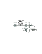
Figure 1: Typical setup for observing two-photon polarization interference for type-II SPDC. NPBS-50/50 nonpolarizing beamsplitter; P1 and P2- linear polarization filters; D1, D2- photodetectors

When the anti-correlation ’dip’ is observed in its polarization version, the experiment is organized as follows (Fig.1). The two-photon light emitted via type-II SPDC under collinear frequency-degenerate phase matching is split in two beams by a non-polarizing beamsplitter, and each of the two beams, after passing through a polarizer, is addressed to a photon counting detector. The output pulses of both detectors are sent to a coincidence circuit, and the coincidence counting rate is measured. There are two basic ways to observe the interference. In one way, the polarizers are fixed at the positions ($45^{\circ},-45^{\circ}$) or ($45^{\circ},45^{\circ}$) and a variable delay is introduced between the photons of a pair. When the delay exactly equals $DL/2$, where $L$ is the crystal length and $D\equiv\frac{1}{u_{o}}-\frac{1}{u_{e}}$ is the inverse group velocity difference between the orthogonally polarized photons of a pair, the coincidence counting rate goes to a minimum or to a maximum, depending on the polarizer settings. The other way to observe the ’dip’ is to fix the delay and to rotate one of the polarizers, the other one being fixed at $45^{\circ}$. This way one obtains an interference pattern with the visibility depending on the e-o delay. When the e-o delay equals $DL/2$, the visibility is maximal and close to $100\%$. This pattern is usually called polarization interference pattern.

The fact that obtaining high-visibility interference requires the e-o delay to be equal to $DL/2$ follows from the following considerations. In a setup as shown in Fig.1, the state at the output of the beamsplitter is

$$|\Psi\rangle=|vac\rangle+\int{d\Omega}F(\Omega)\{a^{\dagger}_{H1}(\omega_{0}+\Omega)a^{\dagger}_{V2}(\omega_{0}-\Omega)e^{i\Omega\tau_{0}}$$

$$+a^{\dagger}_{V1}(\omega_{0}+\Omega)a^{\dagger}_{H2}(\omega_{0}-\Omega)\exp^{-i\Omega\tau_{0}}\}|vac\rangle,$$ (5)

where $a^{\dagger}_{\sigma i}$ are photon creation operators in the horizontal and vertical polarization modes (denoted by $\sigma=H,V$) and two spatial modes (denoted by $i=1,2$); $\omega_{0}=\omega_{p}/2$, $\omega_{p}$ is the pump frequency, and the terms corresponding to both photons of the two-photon state going to the same port of the beamsplitter have been omitted. The difference between the group velocities of signal and idler photons in the non-linear crystal where spontaneous parametric down-conversion is generated, leads to the factors $e^{\pm i\Omega\tau_{0}}$ by the two terms of Eq.(1), with $\tau_{0}=DL/2$.

If one polarizer is fixed at an angle $\theta_{1}$ and the other polarizer, at an angle $\theta_{2}$, then, taking into account the transformation of the photon creation operators, we can write the state after the polarizers in the same way as in Eq.(2), but with the spectral two-photon amplitude $F(\Omega)$ replaced by

$$F^{\prime}(\Omega)=F(\Omega)\{\sin(\theta_{1}+\theta_{2})\cos(\Omega\tau_{0})$$

$$-i\sin(\theta_{1}-\theta_{2})\sin(\Omega\tau_{0})\}.$$ (6)

The second-order correlation function is given by the square modulus of the two-photon amplitude , which can be easily calculated from Eq.(6):

$$F^{\prime}(\tau)=\cos(\theta_{1})\sin(\theta_{2})F(\tau+\tau_{0})$$

$$+\cos(\theta_{2})\sin(\theta_{1})F(\tau-\tau_{0}).$$ (7)

Since the two-photon spectral amplitude for type-II SPDC has the shape

$$F(\Omega)=\frac{\sin(DL\Omega/2)}{DL\Omega/2},$$ (8)

the two-photon amplitude $F(\tau)$ has a rectangular shape with the width $2\tau_{0}$  Rubin . For this reason, the first and the second terms of Eq.(7) do not overlap in time, and no interference can be observed between them in the second-order correlation function. However, it is worth mentioning that the two-photon amplitude $F^{\prime}(\tau)$ indeed has interference structure, and it could be revealed if one were able to measure $F^{\prime}(\tau)$ directly and not its square modulus (the intensity correlation function).

The two cases demonstrating interference most explicitly are the following ones kiess : $\theta_{1}=\theta_{2}=45^{\circ}$ and $\theta_{1}=-45^{\circ},\theta_{2}=45^{\circ}$. For these cases, Eq.(7) gives the following second-order intensity correlation functions:

$$G_{\pm}^{(2)}(\tau)\equiv|F^{\prime}(\tau)_{\pm}|^{2}=\frac{1}{4}|F(\tau-\tau_{0})\pm F(\tau+\tau_{0})|^{2},$$ (9)

where $G_{+}^{(2)}(\tau)$ corresponds to $\theta_{1}=\theta_{2}=45^{\circ}$ and $G_{-}^{(2)}(\tau)$ to $\theta_{1}=-45^{\circ},\theta_{2}=45^{\circ}$ orientations of the polarizers.

To observe the interference, one usually compensates the delay $\tau_{0}=DL/2$ by introducing additional birefringent material after the crystal  Rubin , delay . When $\tau_{0}$ is reduced to zero, the two-photon amplitude in Eq.(7) becomes $F^{\prime}(\tau)=\sin(\theta_{1}+\theta_{2})F(\tau)$ , and the interference with 100% visibility can be observed by fixing one of the polarizers at and rotating the other one.

Apart from compensating the delay, interference can be obtained by using narrowband filters selecting the central part of the spectral amplitude $F(\Omega)$  Rubin . This can be viewed as ’spreading’ the two amplitudes in Eq.(9), to provide an overlap between them.

In the present work, we spread the two-photon amplitudes in Eq.(9) in a different way: not by using narrowband filters but by passing the two-photon radiation through a sufficiently long optical fibre. This, on the one hand, provides the same effect as narrowband filters, in the sense that high-visibility polarization interference can be observed. On the other hand, it allows one to observe the interference structure in the shape of the second-order correlation function, which, due to the propagation of two-photon light through the fibre, becomes very broad.

Indeed, if the biphoton beam, before entering the beamsplitter, passes through a fibre with length $z$ being large enough  sufflength , then, according to (4,9)

$$G_{\pm}^{(2)}(\tau^{\prime})\sim|e^{\frac{i(\tau^{\prime}-\tau_{0})^{2}}{2\tau_{0}\tau_{f}}}\hbox{sinc}(\frac{\tau^{\prime}-\tau_{0}}{\tau_{f}})$$

$$\pm e^{\frac{i(\tau^{\prime}+\tau_{0})^{2}}{2\tau_{0}\tau_{f}}}\hbox{sinc}(\frac{\tau^{\prime}+\tau_{0}}{\tau_{f}})|^{2},$$ (10)

where $\tau^{\prime}\equiv\tau-k^{\prime}z$ is the shifted time and $\tau_{f}\equiv 2k^{\prime\prime}z/\tau_{0}$ is the typical width of the correlation function after the fibre  Krivitsky .

Taking into account that $\tau_{f}>>\tau_{0}$ , one can rewrite Eq.(10) as

$$G_{+}^{(2)}(\tau^{\prime})\sim\frac{\sin^{2}(\tau^{\prime}/\tau_{f})\cos^{2}(\tau^{\prime}/\tau_{f})}{(\tau^{\prime}/\tau_{f})^{2}},$$

$$G_{-}^{(2)}(\tau^{\prime})\sim\frac{\sin^{4}(\tau^{\prime}/\tau_{f})}{(\tau^{\prime}/\tau_{f})^{2}}.$$ (11)

The interference structure of the correlation functions Eq.(11) can be observed if the time resolution of measuring $G^{(2)}(\tau^{\prime})$ is good enough. Two main reasons for the resolution reduction must be considered: the time jitter of the detectors (typically of the order of several hundreds of picoseconds), and the jitter contribution of the electronic technique (amplitude walk and noise) used for the coincidence detection.

The most widely used coincidence detection technique involves direct measurement of the time delay between the photocount pulses of the two detectors by means of a time-to-amplitude converter (TAC), which converts linearly the time interval between the two input pulses (START and STOP) into an output pulse of a proportional amplitude. This analog pulse is forwarded to a multichannel analyzer (MCA), which gives the histogram of the input pulse amplitudes corresponding to the probability distribution for the time interval between the counts of the two detectors. One can show  Mandel that in the limit of small photon fluxes, this time interval distribution coincides in shape with the second-order intensity correlation function. The resolution of such technique could be on the order of one picosecond if the detector jitter time were negligible. Therefore, it is mainly the time jitter of the detectors that sets the resolution of measuring the shape of $G^{(2)}(\tau^{\prime})$. It follows that in order to observe the interference structure, the time spread of the correlation function in the fibre should be much larger than the jitter time of the detectors.

It is interesting to discuss how the correlation function changes if the delay $\tau_{0}$ between the signal and idler photons is changed by placing after the crystal a birefringent plate (for instance, a quartz plate) introducing a delay $\tau_{p}$ with the sign equal or opposite to that of $\tau_{0}$ . Formulas (11) in this case become

$$G_{+}^{(2)}(\tau^{\prime})\sim\frac{\sin^{2}(\tau^{\prime}/\tau_{f})\cos^{2}(\kappa\tau^{\prime}/\tau_{f})}{(\tau^{\prime}/\tau_{f})^{2}},$$

$$G_{-}^{(2)}(\tau^{\prime})\sim\frac{\sin^{2}(\tau^{\prime}/\tau_{f})\sin^{2}(\kappa\tau^{\prime}/\tau_{f})}{(\tau^{\prime}/\tau_{f})^{2}},$$ (12)

where $\kappa=\frac{\tau_{0}+\tau{p}}{\tau_{0}}$ . For instance, if $\tau_{p}=-1/2\tau_{0}$ (the plate compensates only for half of the e-o delay in the crystal ), $\kappa=\frac{1}{2}$ and the modulation period becomes twice larger than in the absence of the plate.

If the delay $\tau_{0}$ is compensated completely, the $G^{(2)}_{-}(\tau^{\prime})$ peak disappears while the peak $G^{(2)}_{+}(\tau^{\prime})$ acquires the same shape as the peak observed without the polarizers.

If the sign of the delay $\tau_{p}$ is the same as that of $\tau_{0}$, the modulation period of the correlation function after the fibre becomes smaller than in the absence of the birefringent plate.

The next two sections are devoted to the experimental observation of these effects.

IV IV. Experimental setup

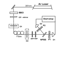
Figure 2: The experimental setup. A cw $Ar^{+}$ laser at 351 nm pumps a type-II BBO crystal; O1, O2- microscope objectives; QWP and HWP- retardation plates; NPBS - 50/50 nonpolarizing beamsplitter; P1 and P2- Glan prisms; D1, D2- avalanche photodiodes. The output of the Start-Stop scheme is analyzed by a multi channel analyzer (MCA).

Two-photon light was generated via spontaneous parametric down-conversion by pumping a type-II 0.5 mm $\beta$-barium borate crystal (BBO) with 0.2 Watt $\hbox{Ar}^{+}$ cw laser beam at the wavelength 351 nm in the collinear frequency-degenerate regime (Fig.2). After the crystal, the pump laser beam was eliminated by a 95% reflecting UV mirror and the SPDC radiation was coupled into a single-mode fibre with the length 240 m or 1 km and the mode field diameter (MFD) of $4\mu$m by a 20x microscope objective lens placed at the distance of 50 cm. This scheme provided imaging of the pump beam waist onto the fibre input with the magnification 1:40. Then, the angle selected by the numerical aperture (NA) of the fibre from the SPDC angular spectrum was $\delta\Theta\approx NA/40=0.006$rad. Without this narrow angular selection, the interference structure would be smeared by contributions from various parts of the SPDC angular spectrum. For the efficient use of the pump beam, the pump was focused into the crystal using a UV-lens with the focal length 30 cm. The resulting beam waist diameter, $120\mu$m, was small enough to be coupled with the fibre core diameter but still sufficiently large not to influence the SPDC angular spectrum.

Because of a rapid polarization drift in the fibre, a quarter-wave plate (QWP) and a half-wave plate (HWP) were introduced after the output of the fibre. These two plates were adjusted to compensate for the random polarization transformation in the fibre and recover the initial horizontal- vertical polarization basis. After the fibre, the biphoton pairs were addressed to a 50/50 nonpolarizing beamsplitter and two photodetection apparatuses, consisting of red-glass filters, pinholes, focusing lenses and avalanche photodiodes (SPCM by EG&G). The photocount pulses of the two detectors, after passing through delay lines, were sent to the START and STOP inputs of a TAC. The output of the TAC was finally addressed to an MCA, and the distribution of coincidences over the time interval between the photocounts of the two detectors, $R_{c}(\tau^{\prime})$, was observed at the MCA output.

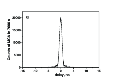
Figure 3: The second-order intensity correlation function of two-photon light after (a) a 240-m fibre and (b) a 1000-m fibre.

The FWHM of the coincidence peak in the absence of the fibre was measured to be approximately 0.8 ns, a value substantially determined by the APD time jitter. In the presence of the fibre, the FWHM of the peak increased, to $1.2$ ns in the case of the $240$ m fibre (Fig.3a) and to $4.5$ ns in the case of the $1000$ m fibre (Fig.3b). The observed distributions were fitted using Eq.(4) with the following fitting parameters: position of the peak, its height, the GVD of the fibre, and the background level caused by accidental coincidences. The obtained GVD values for both fibres used were $3,2\times 10^{-28}$ s²/cm.

The distributions of Fig.3 were obtained without any polarization selection after the beamsplitter. In the main part of the experiment, two polarizers (Glan prisms) were inserted in front of the detectors, and the coincidence distribution was analyzed for the $\theta_{1}=\theta_{2}=45^{\circ}$ and $\theta_{1}=-45^{\circ},\theta_{2}=45^{\circ}$ settings of the polarizers.

V V. Results and discussion

To observe polarization interference in the shape of the correlation function after the fibre, the coincidence distribution at the MCA output was recorded for the two settings of the polarizers considered above, $\theta_{1}=\theta_{2}=45^{\circ}$ and $\theta_{1}=-45^{\circ},\theta_{2}=45^{\circ}$. This measurement was made for two different fibres: a $240$ m one (Fig. 4) and a $1$ km one (Fig. 5). In the case of the $240$ m fibre, the spread of the correlation function was insufficient for providing 100% interference visibility. Indeed, for the width of the correlation function $1.2$ ns and the time resolution of the measurement (determined by the detectors time jitter) $750$ ns, the theory predicts a visibility of $48\%$. (The visibility of polarization interference is obtained from the maximum value in the center of the correlation function in the case of constructive interference ($\theta_{1}=\theta_{2}=45^{\circ}$) and corresponding minimum value in the case of destructive interference ($\theta_{1}=-45^{\circ},\theta_{2}=45^{\circ}$). The experiment showed even less visibility (about 35%), which was probably caused by the polarization drift in the fibre. (Although polarization state of the two-photon light after the fibre was measured and corrected every 10 minutes, polarization drift between these control moments justifies the decrease in the interference visibility from $48\%$ to $35\%$.)

With a $1$ km fibre, the spread of the correlation function ($4.5$ ns) is large enough, so that the interference structure is not significantly smeared by the detectors time jitter (Fig.5). As the settings of the polarization prisms change from $\theta_{1}=\theta_{2}=45^{\circ}$ to $\theta_{1}=-45^{\circ},\theta_{2}=45^{\circ}$, the coincidence counting rate at the center of the correlation function distribution decreases 5.4 times. It means that with a proper selection of the coincidence time window, one can observe high-visibility polarization interference. Indeed, Fig.6 shows the dependence of coincidence counting rate on the orientation of the first polarizer, $\theta_{1}$, with the other polarizer fixed at $\theta_{2}=45^{\circ}$ and only coincidences from a time window of $0.43$ ns (7 MCA channels) near the center of the peak being registered. The visibility of the observed polarization interference fringes is $78\%$. This dependence indicates that by spreading the second-order intensity correlation function and time-selecting it, a Bell state can be produced. To test this we calculated the value of violation of Bell inequality $R\equiv(N(\theta)-N(3\theta))/N(\infty)\leq 0.25$, where $N(\theta)$ is the number of coincidences taken at the relative orientation of polarizers $\theta\equiv\theta_{1}-\theta_{2}$ which have been chosen $\theta=30^{\circ}$ and $N(\infty)$ is the number of coincidences measured without any polarization selection  GenovesePhysRep . After subtracting the accidental coincidences we observed a violation of Bell inequality $R=0.322\pm 0.061$.

As a method of producing a Bell state through SPDC in a type-II crystal, the technique used here is very similar to using narrow-band filters: instead of frequency-selecting the spectral amplitude, here we first Fourier-transform it and then perform time selection. However, if narrow-band filters are used for selecting a Bell state, they are usually centered at the degenerate SPDC frequency. In contrast, in our case, time selection does not have to be performed at the zero time delay. From Eqs.(11) Fig.5, it is clear that high-visibility interference can be also observed at the slopes of the peak or at its side lobes.

For future comparison of the experiment with theoretical predictions, we also measured the correlation function distributions in the case where a birefringent material (quartz) was introduced after the crystal. We used a single quartz plate, with thickness $1$ mm, whose optic axis could be set parallel to the plane containing the optic axis of the BBO crystal or orthogonal to it. In the first case, the quartz plate reduced the e-o delay between the photons of the same pair while in the second case, it increased this delay. The corresponding coincidence distributions obtained in experiment are presented in Figs.7 (a-d). The curves show the theoretical fit with formulas (12).

In all measurements described above, the main difficulty was caused by the rapid polarization drift in the fibre, which considerably smeared the interference structure of the second-order correlation function. To avoid this effect, we have performed a measurement where polarization drift was eliminated, by placing a single polarization prism before the fibre and no prisms after the fibre. Naturally, this way one can only observe the coincidence distribution in the $\theta_{1}=\theta_{2}=45^{\circ}$ configuration, since both polarizers are represented by a single Glan prism fixed at $45^{\circ}$. Coincidence distributions obtained this way are shown in Fig.8: (a) with no plates; (b) with one $1$ mm plate and (c) with two $1$ mm plates inserted after the crystal, their optic axes being orthogonal to the plane of the BBO crystal optic axis. Here it is clearly seen that increasing the e-o delay (by inserting additional plates) leads to a decrease in the oscillation period in the shape of the second-order correlation function. The interference structure observed in Fig.8c has relatively low visibility because the modulation period becomes comparable with the time resolution of the detection system ($750$ ns).

VI VI. Conclusion

In summary, we have studied, both theoretically and experimentally, the polarization interference structure of the second-order intensity correlation function for two-photon light generated via type-II SPDC and fed into a setup for observing the anti-correlation ’dip’ effect. To register this structure, we made the correlation function get spread due to the propagation of the two-photon light through a medium with group-velocity dispersion (in our case, an optical fibre). The interference reveals itself as a peak or a dip in the middle of the coincidence distribution observed at the MCA output. Since the interference structure is caused by the delay between orthogonally polarized photons of a pair accumulated in the course of their propagation through the crystal, increasing or reducing this delay by means of birefringent plates introduced after the crystal considerably changes the structure. This effect has been also observed in the experiment.

The shape of the correlation function after the fibre is given by a scaled square modulus of the two-photon spectral amplitude. One can say that the fibre performs a Fourier transformation of the two-photon amplitude. This fact, already mentioned earlier in the literature  valencia , can be also used for measuring the width of the two-photon amplitude in the cases where it is too narrow to be measured by alternative methods.

It might seem that because the shape of the two-photon amplitude after the fibre repeats, with some scaling factor, the two-photon spectral amplitude before the fiber, the spectrum of two-photon light should reveal the same structure. This, however, is not true, because in our consideration of the state vector (see Eq.(5)) we only included the terms corresponding to the cases where both photons went into different ports of the beamsplitter. At the same time, the spectrum of SPDC is formed by all kinds of pairs, including those going into a single port.

Still, by fixing a time delay in the coincidence distribution after the fibre we effectively fix the frequency offset $\Omega$ for one of the photons of a pair (and for the other one as well). Does it mean that the presented way of observing polarization interference is identical to the one where narrow-band filters are used, selecting the frequencies of the two photons? In principle, the answer is ’yes’. However, in practice, with the time delay selection one can use not only the central part of the coincidence distribution but also its side parts, which is much more difficult to provide with the filters.

It is important to stress that the interference would be present in the two-photon amplitude and hence, in the two-photon spectral amplitude, after the NPBS and the Glan prisms, even without the fibre. However, without the fibre, all that one can measure is the square modulus of the two-photon amplitude, which has no interference structure. Measuring the shape of the two-photon spectral amplitude after the beamsplitter is difficult since it requires spectroscopic and correlation techniques simultaneously. In our work it is done with the help of the fibre: the spread two-photon amplitude reproduces the shape of the spectral amplitude, and is broad enough to be studied with the existing equipment.

Finally, one can mention that the experiment presented here can be considered as a method of preparing (with post-selection) polarization Bell states in the two space modes after the beamsplitter. This fact by itself has little practical importance since Bell-state preparation with two-photon light is a well-developed field of quantum optics and there are tens of various ways to generate Bell states. However, it is worth noting that effects of $G^{(2)}$ spreading will take place whenever two-photon light is propagating through a sufficiently long fibre (which is the case in many quantum communication experiments), and this can be taken into account to simplify the observation of two-photon interference.

This work has been supported by MIUR (FIRB RBAU01L5AZ-002 and RBAU014CLC-002, PRIN 2005023443-002 ), by Regione Piemonte (E14), and by ”San Paolo foundation”, M.Ch. also acknowledges the support of the Russian Foundation for Basic Research, grant no.06-02-16393.

Figure 4: The measured shape of the second-order correlation function in the case of a 240-m fibre and the settings of the polarizers (a) $\theta_{1}=\theta_{2}=45^{\circ}$ and (b) $\theta_{1}=-45^{\circ},\theta_{2}=45^{\circ}$ . Points are experimental data from the MCA output; curves show the theoretical dependencies with an account for the detector jitter time $750$ ns.

Figure 5: The measured shape of the second-order correlation function in the case of a 1-km fibre and the settings of the polarizers (a) $\theta_{1}=\theta_{2}=45^{\circ}$ and (b) $\theta_{1}=-45^{\circ},\theta_{2}=45^{\circ}$ . Points are experimental data from the MCA output; curves show the theoretical dependencies with an account for the detector jitter time $750$ ns.

Figure 6: Coincidence counting rate as a function of the orientation of polarizer 1, with polarizer 2 fixed at $45^{\circ}$ and only coincidences within a 0.43 ns window at the center of the peak being registered.

Figure 7: The measured shape of the second-order correlation function for the case of a quartz plate of thickness 1 mm placed at the output of the crystal with the optic axis parallel to the plane of the BBO optic axis (a,b) and orthogonal to this plane (c,d), for two different settings of the polarizers: $\theta_{1}=\theta_{2}=45^{\circ}$ (a,c) and $\theta_{1}=-45^{\circ},\theta_{2}=45^{\circ}$(b,d). The length of the fibre is 1 km. The curves show the theoretical dependencies using  (12).

Figure 8: The measured shape of the second-order correlation function for the case of (a) no quartz plates, (b) one quartz plate of thickness $1$ mm and (c) two quarts plates of thickness $1$ mm placed at the output of the crystal with the optic axes orthogonal to the plane of the BBO optic axis (which increases the e-o delay), for the case of a single polarizer introduced before the fibre. The polarizer is set at $45^{\circ}$. The length of the fibre is $1$ km. The curves show the theoretical dependencies using  (12).

References

- (1) X. Li, P. Voss, J. Sharping, and P. Kumar, Phys. Rev. Lett. 94, 053601 (2005); J. Fulconis, O. Alibart, W.J. Wadsworth, P. St.J. Russell and J. G. Rarity, Optics Express 13, no. 19757219 (2005); H. Takesue and K. Inoue, Phys. Rev. A 70, 031802 (R) (2004); J. Fan, A. Migdall, and L. J. Wang, Opt. Lett. 30, 3368-3370 (2005).
- (2) G. Brida, M.V. Chekhova, M. Genovese, M. Gramegna, and L.A. Krivitsky, Phys. Rev. Lett. 96, 143601 (2006).
- (3) Y.H. Shih, A.V. Sergienko, M.H. Rubin, T.E. Kiess, and C. O. Alley, Phys. Rev. A 50, 23 (1994).
- (4) Y.H. Shih and A.V. Sergienko, Phys. Rev. A 50, 2564 (1994).
- (5) S. Viciani, A. Zavatta, and M. Bellini, Phys. Rev. A 69, 053801 (2004).
- (6) A.V. Burlakov, M.V. Chekhova, D.N. Klyshko, S.P. Kulik, A.N. Penin, D.V. Strekalov, and Y.H. Shih, Phys. Rev. A 56, 3214 (1997); E.J.S. Fonseca, C.H. Monken, and S. Padua, Phys. Rev. Lett. 82, 2868 (1999); G. Brida et al., Phys. Rev. A 68, 033803 (2003).
- (7) One can provide this by putting small pinholes at a certain distance from the crystal where photon pairs are generated.
- (8) M.V. Chekhova, JETP Lett. 75, 225 (2002).
- (9) A. Valencia, M.V. Chekhova, A.S. Trifonov, and Y.H. Shih, Phys. Rev. Lett. 88, 183601 (2002).
- (10) A.V. Burlakov, M.V. Chekhova, O.A. Karabutova, and S.P. Kulik, Phys. Rev. A 64, 041803 (R) (2001), see also C.K. Hong, Z.Y. Ou, and L. Mandel, Phys. Rev. Lett. 59, 2044 (1987); J.G. Rarity and P.R. Tapster, JOSA B 6, 1221 (1989); A.V. Belinsky and D.N. Klyshko, Laser Phys. 4, 663 (1994).
- (11) A.M. Steinberg, P.G. Kwiat, and R.Y. Chiao, Phys. Rev. Lett. 68, 2421 (1992).
- (12) M.H. Rubin, D.N. Klyshko, Y.H. Shih, and A.V. Sergienko, Phys. Rev. A 50, 5122 (1994).
- (13) P. Kwiat et al. Phys. Rev. Lett. 75, 4337 (1995).
- (14) A typical length of about 1 meter is sufficient.
- (15) L.A. Krivitsky and M.V. Chekhova, JETP Lett. 81, 125 (2005).
- (16) L. Mandel and E. Wolf, Optical Coherence and Quantum Optics (Cambridge University Press, Cambridge, England, 1995).
- (17) M. Genovese, Phys. Rep. 413, no.6, 319 (2005)