Phase-Conjugate Optical Coherence Tomography

Abstract

Quantum optical coherence tomography (Q-OCT) offers a factor-of-two improvement in axial resolution and the advantage of even-order dispersion cancellation when it is compared to conventional OCT (C-OCT). These features have been ascribed to the non-classical nature of the biphoton state employed in the former, as opposed to the classical state used in the latter. Phase-conjugate OCT (PC-OCT), introduced here, shows that non-classical light is not necessary to reap Q-OCT’s advantages. PC-OCT uses classical-state signal and reference beams, which have a phase-sensitive cross-correlation, together with phase conjugation to achieve the axial resolution and even-order dispersion cancellation of Q-OCT with a signal-to-noise ratio that can be comparable to that of C-OCT.

Optical coherence tomography (OCT) produces 3-D imagery through focused-beam scanning (for transverse resolution) and interference measurements (for axial resolution). Conventional OCT (C-OCT) uses classical-state signal and reference beams, with a phase-insensitive cross-correlation, and measures their second-order interference in a Michelson interferometer Schmitt . Quantum OCT (Q-OCT) employs signal and reference beams in an entangled biphoton state, and measures their fourth-order interference in a Hong-Ou-Mandel (HOM) interferometer Abouraddy ; Abouraddy:two . In comparison to C-OCT, Q-OCT offers the advantages of a two-fold improvement in axial resolution and even-order dispersion cancellation. Q-OCT’s advantages have been ascribed to the non-classical nature of the entangled biphoton state, but we will report an OCT configuration that reaps both of these advantages with classical light.

Q-OCT derives its signal and reference beams from spontaneous parametric down-conversion (SPDC), whose outputs are in a zero-mean Gaussian state, with a non-classical phase-sensitive cross-correlation function Sun ; Shapiro:Gaussian . In the low-flux limit, this non-classical Gaussian state becomes a stream of individually detectable biphotons. Classical-state light beams can also have phase-sensitive cross-correlations, but quantum or classical phase-sensitive cross-correlations do not yield second-order interference. This is why fourth-order interference is used in Q-OCT. Our new OCT configuration—phase-conjugate OCT (PC-OCT)—uses phase conjugation to convert a phase-sensitive cross-correlation into a phase-insensitive cross-correlation that can be seen in second-order interference. As we shall see, it is phase-sensitive cross-correlation, rather than non-classical behavior per se, that provides the axial resolution improvement and even-order dispersion cancellation.

The basic block diagram for continuous-wave PC-OCT is shown in Fig. 1, where we have suppressed all spatial coordinates, to focus our attention on the axial behavior, and we have drawn a transmission geometry, whereas the actual system would employ a bistatic geometry in reflection. The signal and reference beams at the PC-OCT input are classical fields with a common center frequency $\omega_{0}$, and baseband complex envelopes, $E_{S}(t)$ and $E_{R}(t)$, with powers $\hbar\omega_{0}|E_{K}(t)|^{2}$, for $K=S,R$. These complex fields are zero-mean, stationary, jointly Gaussian random processes that are completely characterized by their phase-insensitive auto-correlations $\langle E_{K}^{*}(t+\tau)E_{K}(t)\rangle={\cal{F}}^{-1}[S(\Omega)]$, for $K=S,R$, and their phase-sensitive cross-correlation $\langle E_{S}(t+\tau)E_{R}(t)\rangle={\cal{F}}^{-1}[S(\Omega)]$, where

$${\cal{F}}^{-1}[S(\Omega)]\equiv\int_{-\infty}^{\infty}\!\frac{d\Omega}{2\pi}\,S(\Omega)e^{-i\Omega\tau},$$ (1)

is the inverse Fourier transform of $S(\Omega)$, and $S(\Omega)=S(-\Omega)\geq 0$ is the common spectrum of the signal and reference beams at detunings $\pm\Omega$ from $\omega_{0}$. These fields have the maximum phase-sensitive cross-correlation that is consistent with classical physics Sun .

The signal beam is focused on a transverse spot on the sample yielding a reflection with complex envelope $E_{H}(t)=E_{S}(t)\star h(t)$, where $\star$ denotes convolution and $h(t)={\cal{F}}^{-1}[H(\Omega)]$ with

$$H(\Omega)=\int_{0}^{\infty}\!dz\,r(z,\Omega)e^{i2\phi(z,\Omega)}$$ (2)

being the sample’s baseband impulse response. In Eq. (2), $r(z,\Omega)$ is the complex reflection coefficient at depth $z$ and detuning $\Omega$, and $\phi(z,\Omega)$ is the phase acquired through propagation to depth $z$ in the sample. After conjugate amplification, we obtain the complex envelope $E_{C}(t)=[E_{H}^{*}(t)+w(t)]\star\nu(t)$, where $w(t)$, a zero-mean, circulo-complex, white Gaussian noise with correlation function $\langle w^{*}(t+\tau)w(t)\rangle=\delta(\tau)$, is the quantum noise injected by the conjugation process, and $\nu(t)={\cal{F}}^{-1}[V(\Omega)]$ gives the conjugator’s baseband impulse response in terms of its frequency response. The output of the conjugator is refocused onto the sample resulting in the positive-frequency field $E_{1}(t)=[E_{C}(t)\star h(t)]e^{-i\omega_{0}t}$, which is interfered with $E_{2}(t)=E_{R}(t-T)e^{-i\omega_{0}(t-T)}$ in a Michelson interferometer, as shown in Fig. 1.

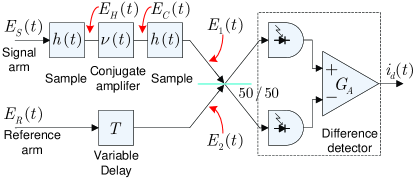
Figure 1: (Color online) Phase-conjugate OCT.

The detectors in Fig. 1 are assumed to have quantum efficiency $\eta$, no dark current, and thermal noise with a white current spectral density $S_{i_{\rm th}}$. The average amplified difference current, which constitutes the PC-OCT signature, is then

$$\langle i_{d}(t)\rangle = 2q\eta G_{A}\,{\rm Re}\!\left(\int_{-\infty}^{\infty}\!\frac{d\Omega}{2\pi}\,H^{*}\!(-\Omega)H(\Omega)\right.$$ (3)

$$\times \left.V^{*}\!(-\Omega)S(\Omega)e^{-i(\Omega-\omega_{0})T}\right),$$

where $q$ is the electron charge.

In C-OCT the signal and reference inputs have complex envelopes that are zero-mean, stationary, jointly Gaussian random processes which are completely characterized by their phase-insensitive auto- and cross-correlations, $\langle E_{J}^{*}(t+\tau)E_{K}(t)\rangle={\cal{F}}^{-1}[S(\Omega)]$, for $J,K=S,R$. As shown in Fig. 2, C-OCT illuminates the sample with the signal beam and interferes the reflected signal—still given by convolution of $E_{S}(t)$ with $h(t)$—with the delayed reference beam in a Michelson interferometer. Here we find that the average amplified difference current is

$$\langle i_{d}(t)\rangle=2q\eta G_{A}$$ (4)

$$\times {\rm Re}\!\left(\int_{-\infty}^{\infty}\!\frac{d\Omega}{2\pi}\,H^{*}\!(-\Omega)S(\Omega)e^{-i(\Omega-\omega_{0})T}\right).$$

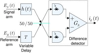
Figure 2: (Color online) Conventional OCT.

For Q-OCT we must use quantum fields, because non-classical light is involved. Now the baseband signal and reference beams are photon-units field operators, $\hat{E}_{S}(t)$ and $\hat{E}_{R}(t)$, with the following non-zero commutators, $[\hat{E}_{J}(t),\hat{E}_{K}^{\dagger}(u)]=\delta_{JK}\delta(t-u)$, for $J,K=S,R$. Q-OCT illuminates the sample with $\hat{E}_{S}(t)$ and then applies the field operator for the reflected beam plus that for the reference beam to an HOM interferometer, as shown in Fig. 3. The familiar biphoton HOM dip can be obtained theoretically—in a manner that is the natural quantum generalization of the classical Gaussian-state analysis we have used so far in this paper Sun —by taking the signal and reference beams to be in a zero-mean joint Gaussian state that is completely characterized by the phase-insensitive (normally-ordered) auto-correlations $\langle\hat{E}_{K}^{\dagger}(t+\tau)\hat{E}_{K}(t)\rangle={\cal{F}}^{-1}[S(\Omega)]$, for $K=S,R$, and the phase-sensitive cross-correlation $\langle\hat{E}_{S}(t+\tau)\hat{E}_{R}(t)\rangle={\cal{F}}^{-1}[\sqrt{S(\Omega)(S(\Omega)+1)}]$. This joint signal-reference state has the maximum possible phase-sensitive cross-correlation permitted by quantum mechanics. In the usual biphoton limit wherein HOM interferometry is performed, $S(\Omega)\ll 1$ prevails, and the average photon-coincidence counting signature can be shown to be

$$\langle C(T)\rangle=\frac{q^{2}\eta^{2}}{2}\left[\int_{-\infty}^{\infty}\!\frac{d\Omega}{2\pi}\,|H(\Omega)|^{2}S(\Omega)\right.$$ (5)

$$- \left.{\rm Re}\!\left(\int_{-\infty}^{\infty}\!\frac{d\Omega}{2\pi}H^{*}\!(-\Omega)H(\Omega)S(\Omega)e^{-i2\Omega T}\right)\right].$$

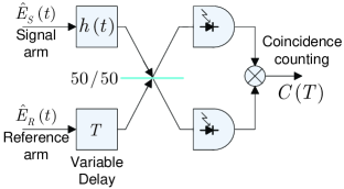
Figure 3: (Color online) Quantum OCT.

Let us assume that $V^{*}(-\Omega)S(\Omega)\approx V^{*}S(\Omega)=(V^{*}P_{S}\sqrt{2\pi/\Omega_{S}^{2}})e^{-\Omega^{2}/2\Omega_{S}^{2}}$ and $H(\Omega)=re^{i(\omega_{0}+\Omega)T_{0}}$, with $|r|\ll 1$. Physically, this corresponds to having a conjugate amplifier whose bandwidth is much broader than that of the signal-reference source, and a sample that is a weakly-reflecting mirror at delay $T_{0}$. Equation (3) then gives a PC-OCT average amplified difference current that, as a function of the reference-arm delay $T$, is a sinusoidal fringe pattern of frequency $\omega_{0}$ with a Gaussian envelope proportional to $e^{-2\Omega_{S}^{2}(T_{0}-T/2)^{2}}$. The average amplified difference current in C-OCT behaves similarly: from Eq. (4) we find that it too is a sinusoidal, frequency-$\omega_{0}$ fringe pattern in $T$, but its envelope is proportional to $e^{-\Omega_{S}^{2}(T_{0}-T)^{2}/2}$. The signature of Q-OCT, found from Eq. (5), is a dip in the average coincidence-count versus reference-arm delay that is proportional to $e^{-2\Omega_{S}^{2}(T_{0}-T)^{2}}$. Defining the axial resolutions of these OCT systems to be the full-width between the $e^{-2}$ attenuation points in their Gaussian envelopes viewed as functions of $T_{0}$ shows that PC-OCT and Q-OCT both achieve factor-of-two improvements over C-OCT for the same source bandwidth.

To probe the effect of dispersion on PC-OCT, C-OCT, and Q-OCT, we modify the sample’s frequency response to $H(\Omega)=re^{i[(\omega_{0}+\Omega)T_{0}+b\Omega^{2}/2]}$, where $b$ is a non-zero real constant representing second-order (group-velocity) dispersion. Because the sample’s frequency response enters the PC-OCT and Q-OCT signatures as $H^{*}(-\Omega)H(\Omega)$, neither one is affected by this dispersion term in $H(\Omega)$, i.e., it cancels out. For C-OCT, however, we find that the Gaussian envelope of the average amplified difference current is now proportional to $e^{-\Omega_{S}^{2}(T_{0}-T)^{2}/2(1+\Omega^{4}_{S}b^{2})}$, i.e., its axial resolution becomes badly degraded when $\Omega_{S}^{4}b^{2}\gg 1$. More generally, for $H(\Omega)=re^{i[(\omega_{0}+\Omega)T_{0}+\beta(\Omega)]}$, PC-OCT and Q-OCT are immune to dispersion created by the even-order terms in the Taylor series expansion of $\beta(\Omega)$.

Having shown that PC-OCT retains the key advantages of Q-OCT, let us turn to its SNR behavior. Because Q-OCT relies on SPDC to generate the entangled biphoton state, and Geiger-mode avalanche photodiodes to perform photon-coincidence counting, its image acquisition is much slower than that of C-OCT, which can use bright sources and linear-mode detectors. To assess the SNR of PC-OCT we shall continue to use the Gaussian spectrum for $S(\Omega)$ and the non-dispersing mirror for $H(\Omega)$, but, in order to limit its quantum noise, we take the conjugator’s frequency response to be $V(\Omega)=Ve^{-\Omega^{2}/4\Omega_{V}^{2}}$. We assume that $i_{d}(t)$ is time averaged for $T_{I}$ sec (denoted $\langle i_{d}(t)\rangle_{T_{I}}$) at the reference-arm delay that maximizes the interference signature, and we define SNR${}_{\text{PC-OCT}}=\langle i_{d}(t)\rangle^{2}/{\rm var}[\langle i_{d}(t)\rangle_{T_{I}}]$. When the $w(t)$ contribution to the conjugator’s output dominates the $E_{H}(t)$ contribution we find that

$${\rm SNR}_{\rm PC-OCT}=$$ (6)

$$\frac{8T_{I}\eta|r|^{4}|V|^{2}P_{S}^{2}\Omega_{V}^{2}/(\Omega_{S}^{2}+2\Omega_{V}^{2})}{\left[\Omega_{\rm th}+P_{S}+|rV|^{2}\sqrt{\Omega_{V}^{2}/2\pi}+\frac{\displaystyle 2\eta|rV|^{2}P_{S}\Omega_{V}}{\sqrt{\displaystyle\Omega_{S}^{2}+\Omega_{V}^{2}}}\,\right]},$$

where $\Omega_{\rm th}\equiv S_{i_{\rm th}}/q^{2}\eta$. From left to right the terms in the noise denominator are the thermal noise, the reference-arm shot noise, the conjugate-amplifier quantum noise, and the intrinsic noise of the signal$\times$reference interference pattern itself. Best performance is achieved when the conjugator gain $|V|^{2}$ is large enough to neglect the first two noise terms, and the input power $P_{S}$ is large enough that the intrinsic noise greatly exceeds the conjugator’s quantum noise. In this case we get

$${\rm SNR}_{\text{PC-OCT}}=\frac{4T_{I}|r|^{2}P_{S}\Omega_{V}\sqrt{\Omega_{S}^{2}+\Omega_{V}^{2}}}{\Omega_{S}^{2}+2\Omega_{V}^{2}}.$$ (7)

To compare the preceding SNR to that for C-OCT, we define ${\rm SNR}_{\text{C-OCT}}=\langle i_{d}(t)\rangle^{2}/{\rm var}[\langle i_{d}(t)\rangle_{T_{I}}]$ for the Fig. 2 configuration at the peak of the C-OCT interference signature. When the reflected signal field is much weaker than the reference field, we then find that

$${\rm SNR}_{\text{C-OCT}}=4\eta T_{I}|r|^{2}P_{S},$$ (8)

which can be smaller than the ultimate ${\rm SNR}_{\text{PC-OCT}}$ result. However, if PC-OCT’s conjugator gain is too low to reach this ultimate performance, but its reference-arm shot noise dominates the other noise terms, we get

$${\rm SNR}_{\text{PC-OCT}}=\frac{8\eta T_{I}|r|^{4}|V|^{2}P_{S}\Omega_{V}^{2}}{\Omega_{S}^{2}+2\Omega_{V}^{2}},$$ (9)

which is substantially lower than ${\rm SNR}_{\text{C-OCT}}$, because $|rV|^{2}\ll 1$ is implicit in our assumption that the reference shot noise is dominant as high detector quantum efficiency can be expected. Thus we can conclude that PC-OCT will have SNR similar to that of C-OCT, but only if high-gain phase conjugation is available SNRnote .

At this juncture it is worth emphasizing the fundamental physical point revealed by the preceding analysis. The use of entangled biphotons and fourth-order interference measurement in an HOM interferometer enable Q-OCT’s two performance advantages over C-OCT: a factor-of-two improvement in axial resolution and cancellation of even-order dispersion Abouraddy ; Abouraddy:two . Classical phase-sensitive light also produces an HOM dip with even-order dispersion cancellation, but this dip is essentially unobservable because it rides on a much stronger background term Sun . Thus the non-classical character of the entangled biphoton is the source of Q-OCT’s benefits, from which it might be concluded that non-classical light is required for any OCT configuration with these performance advantages over C-OCT. Such is not the case, however, because our PC-OCT configuration shows that it is really phase-sensitive cross-correlations that are at the root of axial resolution enhancement and even-order dispersion cancellation. Phase-sensitive cross-correlations cannot be seen in the second-order interference measurements used in C-OCT. PC-OCT therefore phase conjugates one of the phase-sensitive cross-correlated beams, converting their phase-sensitive cross-correlation into a phase-insensitive cross-correlation that can be seen in second-order interference. Our treatment of PC-OCT assumed classical-state light, and, because we need $S(0)\gg 1$ for high-SNR PC-OCT operation, little further can be expected in the way of performance improvement by using non-classical light in PC-OCT. This can be seen by comparing the cross-spectra $S(\Omega)$ and $\sqrt{S(\Omega)(S(\Omega)+1)}$ when $S(\Omega)=(P_{S}\sqrt{2\pi/\Omega_{S}^{2}})e^{-\Omega^{2}/2\Omega_{S}^{2}}$ with $P_{S}\sqrt{2\pi/\Omega_{S}^{2}}\gg 1$.

The intimate physical relation between PC-OCT and Q-OCT can be further elucidated by considering the way in which the sample’s frequency response enters their measurement averages. We again assume $V^{*}(-\Omega)S(\Omega)\approx V^{*}S(\Omega)$, so that both imagers yield signatures $\propto\int\!d\Omega\,H^{*}(-\Omega)H(\Omega)S(\Omega)$. Abouraddy et al. Abouraddy use Klyshko’s advanced-wave interpretation Klyshko to account for the $H^{*}(-\Omega)H(\Omega)$ factor in the Q-OCT signature as the product of an actual sample illumination and a virtual sample illumination. In our PC-OCT imager, this same $H^{*}(-\Omega)H(\Omega)$ factor comes from the two sample illuminations, one before phase conjugation and one after. In both cases, it is the phase-sensitive cross-correlation that is responsible for this factor. Q-OCT uses non-classical light and fourth-order interference while PC-OCT can use classical light and second-order interference to obtain the same sample information.

That PC-OCT’s two sample illuminations provide an axial resolution advantage over C-OCT leads naturally to considering whether C-OCT would also benefit from two sample illuminations. Consider the Fig. 1 system with $E_{S}(t)$ and $E_{R}(t)$ arising from a C-OCT light source, and the phase-conjugate amplifier replaced with a conventional phase-insensitive amplifier of field gain $G(\Omega)=Ge^{-\Omega^{2}/4\Omega_{G}^{2}}$ with $|G|\gg 1$. This two-pass C-OCT arrangement then yields an interference signature $\propto e^{-2\Omega_{S}^{2}(T_{0}-T/2)^{2}}$ for the weakly-reflecting mirror when the amplifier is sufficiently broadband, and an SNR given by Eq. (6) with $V$ replaced by $G$ and $\Omega_{V}$ replaced by $\Omega_{G}$. Thus two-pass C-OCT has the same axial resolution advantage and SNR behavior as PC-OCT. However, instead of providing even-order dispersion cancellation, two-pass C-OCT doubles all the even-order dispersion coefficients.

Let us conclude by briefly addressing the implementation issues that arise with PC-OCT. Our imager requires: signal and reference light beams with a strong and broadband phase-sensitive cross-correlation; an illumination setup in which the signal beam is focused on and reflected from a sample, undergoes conjugate amplification, is refocused onto the same sample, and then interfered with the time-delayed reference beam; and a broadband, high-gain phase conjugator. Strong signal and reference beams that have a phase-sensitive cross-correlation can be produced by splitting a single laser beam in two, and then imposing appropriate amplitude and phase noises on these beams through electro-optic modulators. Existing optical telecommunication modulators, however, do not have sufficient bandwidth for high-resolution OCT. A better approach to the PC-OCT source problem is to exploit nonlinear optics. SPDC can have THz phase-matching bandwidths, and might be suitable for the PC-OCT application. Unlike Q-OCT, which relies on SPDC for its entangled biphotons, a down-conversion source for PC-OCT can—and should—be driven at maximum pump strength, i.e., there is no need to limit its photon-pair generation rate so that these biphoton states are time-resolved by the $\sim$MHz bandwidth single-photon detectors that are used in Q-OCT’s coincidence counter. Hence pulsed pumping will surely be needed. SPDC is also a possibility for the phase conjugation operation. In a frequency-degenerate type-II phase matched down-converter, the reflected signal $E_{H}(t)$ is applied in one input polarization (call it the signal polarization) and a vacuum state field in the other (idler) polarization. The idler output then has the characteristics needed for PC-OCT, viz., it consists of a phase-conjugated version of the signal input plus the minimum quantum noise needed to preserve free-field commutator brackets Shapiro:Gaussian . Similar phase-conjugate operation can also be obtained from frequency-degenerate four-wave mixing Fisher ; Feinberg ; Norman . In both cases, pulsed operation will be needed to achieve the gain-bandwidth product for high-performance PC-OCT.

In summary, we have a phase-conjugate OCT imager that combines many of the best features of conventional OCT and quantum OCT. Like C-OCT, PC-OCT relies on second-order interference in a Michelson interferometer. Thus it can use linear-mode avalanche photodiodes (APDs), rather than the lower bandwidth and less efficient Geiger-mode APDs employed in Q-OCT. Like Q-OCT, PC-OCT enjoys a factor-of-two axial resolution advantage over C-OCT, and automatic cancellation of even-order dispersion terms. The source of these advantages, for both Q-OCT and PC-OCT, is the phase-sensitive cross-correlation between the signal and reference beams. In PC-OCT, however, this cross-correlation need not be beyond the limits of classical physics, as is required for Q-OCT. Finally, PC-OCT may achieve an SNR comparable to that of C-OCT, thus realizing much faster image acquisition than is currently possible in Q-OCT. All of these PC-OCT benefits are contingent on developing an appropriate source for producing signal and reference light beams with a strong and broadband phase-sensitive cross-correlation, and a phase conjugation system with suitably high gain-bandwidth product.

- (1) J. M. Schmitt, J. Sel. Top. in Quantum Electron. 5, 1205 (1999).
- (2) A. F. Abouraddy, M. B. Nasr, B. E. A. Saleh, A. V. Sergienko and M. C. Teich, Phys. Rev. A 65, 053817 (2002).
- (3) M. B. Nasr, B. E. A. Saleh, A. V. Sergienko and M. C. Teich, Phys. Rev. Lett. 91, 083601 (2003).
- (4) J. H. Shapiro and K.-X. Sun, J. Opt. Soc. Am. B 11, 1130 (1994).
- (5) J. H. Shapiro, Proc. SPIE 5111, 382 (2003).
- (6) Some care should be exercised in making this SNR comparison, because is the total power that illuminates the sample in C-OCT, but it is only the initial sample illumination power in PC-OCT, i.e., there is also the power that illuminates the sample after the phase-conjugation operation.
- (7) D. N. Klyshko, Usp. Fiz. Nauk 154, 133 (1988) [Sov. Phys. Usp. 31, 74 (1988)].
- (8) R. A. Fisher, Opt. Lett. 8, 611(1983).
- (9) J. Feinberg, Opt. Lett. 8, 569 (1983).
- (10) J. B. Norman, Am. J. Phys. 60, 212 (1992).