Proposed realization of the Dicke-model quantum phase transition
in an optical cavity QED system

Abstract

The Dicke model consisting of an ensemble of two-state atoms interacting with a single quantized mode of the electromagnetic field exhibits a zero-temperature phase transition at a critical value of the dipole coupling strength. We propose a scheme based on multilevel atoms and cavity-mediated Raman transitions to realise an effective Dicke system operating in the phase transition regime. Output light from the cavity carries signatures of the critical behavior which is analyzed for the thermodynamic limit where the number of atoms is very large.

I Introduction

The interaction of an ensemble of $N$ two-level atoms with a single mode of the electromagnetic field is a classic problem in quantum optics and continues to provide a fascinating avenue of research in a variety of contexts. The simplest model of this interaction is provided by the Dicke Hamiltonian Dicke54 , which takes the form ($\hbar=1$)

$$\hat{H}=\omega\hat{a}^{\dagger}\hat{a}+\omega_{0}\hat{J}_{z}+\frac{\lambda}{\sqrt{N}}\left(\hat{a}^{\dagger}+\hat{a}\right)\left(\hat{J}_{+}+\hat{J}_{-}\right),$$ (1)

where $\omega_{0}$ is the frequency splitting between the atomic levels, $\omega$ is the frequency of the field mode, and $\lambda$ is the dipole coupling strength. The boson operators $\{\hat{a},\hat{a}^{\dagger}\}$ are annihilation and creation operators for the field, and $\{\hat{J}_{\pm},\hat{J}_{z}\}$ are collective atomic operators satisfying angular momentum commutation relations,

$$\left[\hat{J}_{+},\hat{J}_{-}\right]=2\hat{J}_{z},\qquad\left[\hat{J}_{\pm},\hat{J}_{z}\right]=\mp\hat{J}_{\pm}.$$ (2)

Contained within the possible solutions to this model are a number of significant and topical phenomena, including:

1. A zero-temperature phase transition in the thermodynamic limit, $N\rightarrow\infty$, occurring at the critical coupling strength $\lambda_{\rm c}=\sqrt{\omega\omega_{0}}/2$. For larger than the critical coupling the system enters a super-radiant phase Hepp73a ; Hepp73b ; Wang73 ; Hioe73 ; Carmichael73 ; Duncan74 ; Emary03a ; Emary03b .

2. An associated change in level statistics, indicating a change from “quasi-integrable” to “quantum chaotic” behavior Emary03a ; Emary03b .

3. Critical behavior of the atom-field entanglement, which diverges at the critical point for $N\rightarrow\infty$ Lambert04a ; Lambert05 ; Reslen05 .

It follows that the Dicke model offers a potential setting for investigations of quantum critical behavior, quantum chaos, and quantum entanglement.

Practical realization of a system exhibiting the mentioned phenomena presents something of a problem, however, in that, in familiar quantum-optical systems, the frequencies $\omega$ and $\omega_{0}$ typically exceed the dipole coupling strength by many orders of magnitude. This means that the counter-rotating terms, $\hat{a}^{\dagger}\hat{J}_{+}$ and $\hat{a}\hat{J}_{-}$ in Eq. (1), have very little effect on the dynamics; indeed, they are usually neglected in the so-called “rotating-wave approximation.” Furthermore, dissipation due to atomic spontaneous emission and cavity loss is usually unavoidable, significantly altering the pure Hamiltonian evolution. Hence, it remains as a challenge to provide a practical physical system which might exhibit the interesting behavior associated with the idealized Dicke model.

We propose such a physical system in this paper. We suggest a scheme based on interactions in cavity quantum electrodynamics (cavity QED) which realizes an effective Dicke Hamiltonian (1) with parameters $\omega_{0}\simeq\omega\simeq\lambda$ that are adjustable and can in principle far exceed all dissipation rates. Our scheme uses cavity-plus-laser mediated Raman transitions between a pair of stable atomic ground states, thereby avoiding spontaneous emission. While cavity loss cannot be similarly avoided, it should be possible to achieve cavity QED conditions in which the dissipation rate from the cavity mode is much less than the parameters of the Dicke model.

In fact, the presence of cavity loss constitutes an important and essential aspect of the work presented here: output light from the cavity provides a readily measurable signal from which an experimenter can learn, rather directly, about the properties of the system. In particular, various spectral measurements made on the output light clearly reveal the critical behavior of the Dicke model as the coupling parameter is changed.

We begin in Sec. II with a description of the proposed scheme for realizing the Dicke model in an optical cavity QED system. In Sec. III, we briefly discuss a possible experimental scenario involving atoms confined within a ring cavity and establish parameter values for use in the numerical calculations. Our theoretical study of the dissipative Dicke model in the thermodynamic limit is presented in Sec. IV. It is based upon a linearized analysis in the Holstein-Primakoff representation of the collective atomic spin and the input-output theory of open quantum-optical systems. We present results for the cavity fluorescence spectrum, the probe transmission spectrum, and the spectra of quadrature fluctuations—i.e., homodyne, or squeezing spectra. These spectra vividly illustrate the changing nature of the system through the critical region of the phase transition. We also describe a means of computing variance-based measures of atom-field entanglement from homodyne spectra of the cavity output field. We finish in Sec. V with the conclusion and a discussion of possible further investigations.

II Proposed realization: balanced Raman channels

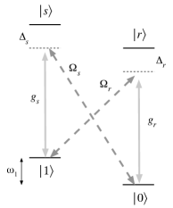
Figure 1: Atomic level scheme. Excited states have energies $\hbar\omega_{j}$ ($j=r,s$). Such a scheme might be realized, e.g., by alkali atoms, with $|0\rangle$ and $|1\rangle$ as different ground-state sublevels. Note that $|r\rangle$ and $|s\rangle$ may be the same level, provided that the Raman channels remain distinct (which requires $\omega_{1}\neq 0$).

We consider an ensemble of $N$ atoms coupled simultaneously to the quantized field of an optical cavity mode and the classical field of a pair of lasers. All fields are co-propagating (in the $x$ direction) TEM₀₀ traveling waves, with beam waists sufficiently broad compared to the atomic ensemble that uniform atom-field coupling strengths may be assumed. Each atom has two stable ground states, $\left|0\right\rangle$ and $\left|1\right\rangle$, which are coupled through a pair of Raman channels, as shown in Fig. 1; specifically, the lasers drive ground-to-excited-state transitions $\left|1\right\rangle\leftrightarrow\left|r\right\rangle$ and $\left|0\right\rangle\leftrightarrow\left|s\right\rangle$ with Rabi frequencies $\Omega_{r}$ and $\Omega_{s}$, respectively, while the cavity mode mediates the $\left|r\right\rangle\leftrightarrow\left|0\right\rangle$ and $\left|s\right\rangle\leftrightarrow\left|1\right\rangle$ transitions, with dipole coupling strengths $g_{r}$ and $g_{s}$. The detunings from the excited states are $\Delta_{r}$ and $\Delta_{s}$, as shown on the figure.

With the inclusion of spontaneous emission and cavity loss, the master equation for the system density operator, $\rho_{\rm sys}$, is written as

$$\dot{\rho}_{\rm sys}=-i\left[\hat{H}_{\rm sys},\rho_{\rm sys}\right]+\mathcal{L}_{\rm cav}\rho_{\rm sys}+\mathcal{L}_{\rm spon}\rho_{\rm sys},$$ (3)

where $\hat{H}_{\rm sys}$ is a sum of Hamiltonians:

$$\hat{H}_{\rm cav}=\omega_{\rm cav}\hat{a}^{\dagger}\hat{a},$$ (4a)

for the cavity oscillator,

$$\hat{H}_{\rm at} = \sum_{j=1}^{N}\left\{\right.\omega_{r}\left|r_{j}\right\rangle\left\langle r_{j}\right|+\omega_{s}\left|s_{j}\right\rangle\left\langle s_{j}\right|+\omega_{1}\left|1_{j}\right\rangle\left\langle 1_{j}\right|$$ (4b)

$$+\left.\left[(\Omega_{r}/2)e^{-i\omega_{lr}t}\left|r_{j}\right\rangle\left\langle 1_{j}\right|e^{ik_{r}x_{j}}+(\Omega_{s}/2)e^{-i\omega_{ls}t}\left|s_{j}\right\rangle\left\langle 0_{j}\right|e^{ik_{s}x_{j}}+\textrm{H.c.}\right]\right\},$$

for the driven atoms (H.c. denotes the Hermitian conjugate), and

$$\hat{H}_{\rm int} = \sum_{j=1}^{N}\left[\left(g_{r}\left|r_{j}\right\rangle\left\langle 0_{j}\right|\hat{a}+g_{s}\left|s_{j}\right\rangle\left\langle 1_{j}\right|\hat{a}\right)e^{ikx_{j}}+\textrm{H.c.}\right],$$ (4c)

for the atom-cavity interaction, where $\omega_{r}$, $\omega_{s}$, and $\omega_{1}$ are atomic frequencies (see Fig. 1), $\omega_{lr}$ and $\omega_{ls}$ are the laser frequencies, and $x_{j}$ locates the $j$-th atom in the traveling waves, which have wavenumbers $k_{r}$, $k_{s}$, and $k$ (where $k_{r}\simeq k_{s}\simeq k$). Cavity loss is included through the Lindblad term

$$\mathcal{L}_{\rm cav}\rho_{\rm sys} = \kappa\left(2\hat{a}\rho_{\rm sys}\hat{a}^{\dagger}-\hat{a}^{\dagger}\hat{a}\rho_{\rm sys}-\rho_{\rm sys}\hat{a}^{\dagger}\hat{a}\right),$$ (5)

and spontaneous emission through the second Lindblad term $\mathcal{L}_{\rm spon}\rho_{\rm sys}$.

From this full master equation a simplified equation is derived by neglecting spontaneous emission and adiabatically eliminating the atomic excited states. We first transform to the interaction picture, introducing the unitary transformation $\hat{U}(t)=\exp(-i\hat{H}_{0}t)$, with

$$\hat{H}_{0}=(\omega_{ls}-\omega_{1}^{\prime})\hat{a}^{\dagger}\hat{a}+\sum_{j=1}^{N}\left\{(\omega_{lr}+\omega_{1}^{\prime})\left|r_{j}\right\rangle\left\langle r_{j}\right|+\omega_{ls}\left|s_{j}\right\rangle\left\langle s_{j}\right|+\omega_{1}^{\prime}\left|1_{j}\right\rangle\left\langle 1_{j}\right|\right\},$$ (6)

where $\omega_{1}^{\prime}$ is a frequency close to $\omega_{1}$, satisfying

$$\omega_{ls}-\omega_{lr}=2\omega_{1}^{\prime}.$$ (7)

Then assuming large detunings of the fields from the excited states,

$$\left|\Delta_{r,s}\right|\gg\Omega_{r,s},\,g_{r,s},\,\kappa,\,\delta_{\rm cav},\,\gamma,$$ (8)

where $\gamma$ the excited state linewidth and

$$\Delta_{r} = \omega_{r}-\left(\omega_{lr}+\omega_{1}^{\prime}\right),\qquad\Delta_{s}=\omega_{s}-\omega_{ls},$$ (10)

$$\quad\delta_{\rm cav}=\omega_{\rm cav}-\left(\omega_{ls}-\omega_{1}^{\prime}\right),$$

we make the adiabatic elimination and neglect constant energy terms to arrive at the simplified master equation for the collective coupling of the ground states $\left|0\right\rangle$ and $\left|1\right\rangle$,

$$\dot{\rho}=-i\left[\hat{H},\rho\right]+{\cal L}_{\rm cav}\rho,$$ (11)

with

$$\hat{H} = \omega\hat{a}^{\dagger}\hat{a}+\omega_{0}\hat{J}_{z}+\delta\hat{a}^{\dagger}\hat{a}\hat{J}_{z}+\frac{\lambda_{r}}{\sqrt{N}}\left(\hat{a}\hat{J}_{+}+\hat{a}^{\dagger}\hat{J}_{-}\right)$$ (12)

$$+\frac{\lambda_{s}}{\sqrt{N}}\left(\hat{a}^{\dagger}\hat{J}_{+}+\hat{a}\hat{J}_{-}\right),$$

where

$$\hat{J}_{+}\equiv\sum_{j=1}^{N}\left|1_{j}\right\rangle\left\langle 0_{j}\right|,\qquad\hat{J}_{-}\equiv\sum_{j=1}^{N}\left|0_{j}\right\rangle\left\langle 1_{j}\right|,$$ (13a)

$$\hat{J}_{z}\equiv\frac{1}{2}\sum_{j=1}^{N}\left(\left|1_{j}\right\rangle\left\langle 1_{j}\right|-\left|0_{j}\right\rangle\left\langle 0_{j}\right|\right)$$ (13b)

are collective atomic operators satisfying commutation relations (2), and the remaining parameters of the model are defined by

$$\omega = \tfrac{1}{2}N(g_{r}^{2}/\Delta_{r}+g_{s}^{2}/\Delta_{s})+\delta_{\rm cav},$$ (14a)

$$\omega_{0} = \tfrac{1}{4}\left(\Omega_{r}^{2}/\Delta_{r}-\Omega_{s}^{2}/\Delta_{s}\right)+\left(\omega_{1}-\omega_{1}^{\prime}\right),$$ (14b)

$$\delta = g_{r}^{2}/\Delta_{r}-g_{s}^{2}/\Delta_{s},$$ (14c)

$$\lambda_{r} = \tfrac{1}{2}\sqrt{N}g_{r}\Omega_{r}/\Delta_{r},$$ (14d)

$$\lambda_{s} = \tfrac{1}{2}\sqrt{N}g_{s}\Omega_{s}/\Delta_{s}.$$ (14e)

With these parameters chosen such that

$$g_{r}^{2}/\Delta_{r}=g_{s}^{2}/\Delta_{s},\qquad g_{r}\Omega_{r}/\Delta_{r}=g_{s}\Omega_{s}/\Delta_{s},$$ (15)

$\hat{H}$ is put into the form of the Dicke Hamiltonian (1),

$$\hat{H}=\omega\hat{a}^{\dagger}\hat{a}+\omega_{0}\hat{J}_{z}+\frac{\lambda}{\sqrt{N}}\left(\hat{a}+\hat{a}^{\dagger}\right)\left(\hat{J}_{+}+\hat{J}_{-}\right),$$ (16)

with

$$\omega = Ng_{r}^{2}/\Delta_{r}+\delta_{\rm cav},$$ (17a)

$$\omega_{0} = \omega_{1}-\omega_{1}^{\prime},$$ (17b)

$$\lambda = \tfrac{1}{2}\sqrt{N}g_{r}\Omega_{r}/\Delta_{r}.$$ (17c)

Hence, we arrive at a realization of the Dicke model with parameters that can be controlled through the laser frequencies and intensities, and where the characteristic energy scales are no longer those of optical photons and dipole coupling but those associated with light shifts and Raman transition rates.

III Potential experimental scheme

Before proceeding with our theoretical analysis, we pause briefly to outline a possible experimental implementation of the proposed model. We imagine the ensemble of atoms confined inside a ring cavity where it interacts with the quantized cavity mode (field operator $\hat{a}$) as shown in Fig. 2(a). The cavity mode copropagates with the two laser fields (Rabi frequencies $\Omega_{r}$ and $\Omega_{s}$) through the ensemble as indicated on the figure by the dashed line. Quantized inputs and outputs are assumed significant through one cavity mirror only—field operators $\hat{a}_{\rm in}$ and $\hat{a}_{\rm out}$ in the figure.

The atomic excitation scheme might be based on an $F=1\leftrightarrow F^{\prime}=1$ transition, as occurs, for example, in ⁸⁷Rb. Such a scheme differs slightly from that of Fig. (1) and is illustrated in Fig. 2(b). The cavity mode is linearly polarized along an axis perpendicular to an applied magnetic field of strength $B$. The magnetic field splits the $m_{F}=\pm 1$ sublevels of the $F=1$ ground state, allowing for the excitation of the distinct Raman channels shown Wilk06 .

Parameter values $g_{r}/2\pi\simeq 50~{}\textrm{kHz}$, $\kappa/2\pi\simeq 20~{}\textrm{kHz}$, and $N\simeq 10^{6}$ appear to be practical Kruse03 ; Nagorny03 ; thus, with the choice $\Omega_{r}/\Delta_{r}=0.005$, one finds an effective coupling strength $\lambda/2\pi=\frac{1}{2}\sqrt{N}g_{r}\Omega_{r}/2\pi\Delta_{r}\simeq 125~{}\textrm{kHz}$. This is significantly larger than the decay rate $\kappa$, placing the system firmly in a regime where the Hamiltonian dynamics can be expected to dominate. Note further that, for these parameters, the spontaneous emission rate due to off-resonant excitation of the atomic excited states is estimated at $\frac{1}{4}(\gamma/2\pi)(\Omega_{r}/\Delta_{r})^{2}\lesssim 40~{}\textrm{Hz}$, where $\gamma/2\pi=6~{}\textrm{MHz}$ has been assumed. Finally, the condition $\omega\simeq\omega_{0}\simeq\lambda$ can be achieved with appropriate choices of the laser and cavity mode frequencies, and ground-state level shifts of the order of $2\pi\cdot$10-15 MHz ($\gtrsim 100\lambda$) would satisfy the requirement for distinct Raman channels.

The above set of parameters provides just one example of the possibilities, and a wide variety of parameter combinations satisfy the requirements of our model. In what follows we concentrate in large part, for numerical investigations, on the set of (normalized) parameters $\{\omega,\omega_{0},\kappa\}=\{1,1,0.2\}$. This choice serves to highlight the main physical features of the model proposed.

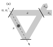
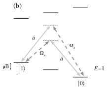
Figure 2: (a) Ring cavity configuration for implementing the proposed realization of the Dicke model. Quantized input and output fields are denoted by $\hat{a}_{\rm in}$ and $\hat{a}_{\rm out}$, respectively. (b) Possible atomic excitation scheme based upon an $F=1\leftrightarrow F^{\prime}=1$ atomic transition and a linearly-polarized cavity field $\hat{a}$. Note that the magnetic field splittings of the Zeeman sublevels are not drawn to scale; the detunings of the optical fields from the excited atomic states are much larger than the ground-state splittings (i.e., $|\Delta_{r,s}|\gg|\mu B|$).

IV Analysis in the Thermodynamic limit

We aim to make a theoretical analysis of the Dicke-model quantum phase transition in the thermodynamic limit, i.e., for $N\gg 1$. Our starting point is a semiclassical analysis of the steady state and its bifurcations, to which a linearized treatment of quantum fluctuations is added using the Holstein-Primakov representation and the input-output theory of open quantum systems.

IV.1 Semiclassical steady states

Introducing the $c$-number variables

$$\alpha\equiv\langle\hat{a}\rangle,\qquad\beta\equiv\langle\hat{J}_{-}\rangle,\qquad w\equiv\langle\hat{J}_{z}\rangle,$$ (18)

where $\alpha$ and $\beta$ are the complex field and atomic polarization amplitudes, respectively, and $w$ is the (real) population inversion, we examine the semiclassical equations of motion

$$\dot{\alpha} = -(\kappa+i\omega)\alpha-i\frac{\lambda}{\sqrt{N}}(\beta+\beta^{\ast}),$$ (19a)

$$\dot{\beta} = -i\omega_{0}\beta+2i\frac{\lambda}{\sqrt{N}}(\alpha+\alpha^{\ast})w,$$ (19b)

$$\dot{w} = i\frac{\lambda}{\sqrt{N}}(\alpha+\alpha^{\ast})(\beta-\beta^{\ast}).$$ (19c)

These follow from master equation (11), with Hamiltonian (16) and cavity damping (5), by neglecting quantum fluctuations and imposing the factorization

$$\langle\left(\hat{a}+\hat{a}^{\dagger}\right)\hat{J}_{z}\rangle \rightarrow \langle\left(\hat{a}+\hat{a}^{\dagger}\right)\rangle\langle\hat{J}_{z}\rangle,$$

$$\langle\left(\hat{a}+\hat{a}^{\dagger}\right)(\hat{J}_{-}-\hat{J}_{+})\rangle \rightarrow \langle\left(\hat{a}+\hat{a}^{\dagger}\right)\rangle\langle(\hat{J}_{-}-\hat{J}_{+})\rangle.$$

The semiclassical equations conserve the magnitude of pseudo angular momentum,

$$w^{2}+\left|\beta\right|^{2}=N^{2}/4.$$ (20)

We use this conservation law and solve Eqs. (19a)–(19c) for the steady states, whence a critical value of the coupling strength occurs at

$$\lambda=\lambda_{\rm c}\equiv\frac{1}{2}\sqrt{(\omega_{0}/\omega)(\kappa^{2}+\omega^{2})}.$$ (21)

For $\lambda<\lambda_{\rm c}$, there are two steady states,

$$\alpha_{\rm ss}=\beta_{\rm ss}=0,\qquad w_{\rm ss}=\pm N/2,$$ (22)

where the states with negative and positive inversion are dynamically stable and unstable, respectively. Both states become unstable for $\lambda>\lambda_{\rm c}$, where the new stable steady states are

$$\alpha_{\rm ss} = \pm\sqrt{N}\frac{\lambda}{\omega-i\kappa}\sqrt{1-\lambda_{\rm c}^{4}/\lambda^{4}}\,,$$ (23a)

$$\beta_{\rm ss} = \mp\frac{N}{2}\sqrt{1-\lambda_{\rm c}^{4}/\lambda^{4}}\,,$$ (23b)

$$w_{\rm ss} = -\frac{N}{2}\lambda_{\rm c}^{2}/\lambda^{2}.$$ (23c)

These quantities are plotted as a function of the coupling strength in Fig. 3. Note the bifurcation to states of finite amplitude and inversion at $\lambda=\lambda_{c}$. This is the Dicke-model quantum phase transition Hepp73a ; Hepp73b ; Wang73 ; Hioe73 ; Carmichael73 ; Duncan74 ; Emary03a ; Emary03b as encountered, without fluctuations, in the thermodynamic limit.

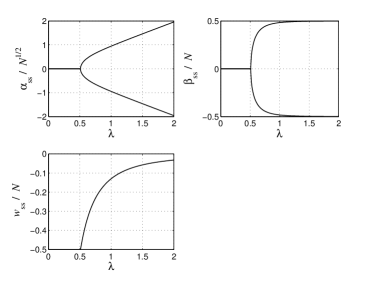
Figure 3: Steady-state field amplitude, $\alpha_{\rm ss}$, polarization amplitude, $\beta_{\rm ss}$, and atomic inversion, $w_{\rm ss}$, plotted as a function of the coupling strength $\lambda$, for $\omega=\omega_{0}=1$ and $\kappa=0.2$. Only stable steady states are shown.

IV.2 Linearized treament of quantum fluctuations in the Holstein-Primakoff representation

In the thermodynamic limit, $N\gg 1$, the quantum fluctuations are small and may be treated in a linearized approach. We follow Emary and Brandes Emary03a ; Emary03b ; Lambert04a ; Lambert05 and make use of the Holstein-Primakoff representation of angular momentum operators Holstein40 ; Ressayre75 . Collective atomic operators $\hat{J}_{+}$, $\hat{J}_{-}$, and $\hat{J}_{z}$ are expressed in terms of annihilation and creation operators, $\hat{b}$ and $\hat{b}^{\dagger}$, of a single bosonic mode:

$$\hat{J}_{+} = \hat{b}^{\dagger}\sqrt{N-\hat{b}^{\dagger}\hat{b}},\qquad\hat{J}_{-}=\hat{J}_{+}^{\dagger},$$ (24a)

$$\hat{J}_{z} = \hat{b}^{\dagger}\hat{b}-N/2,$$ (24b)

from which, using $[\hat{b},\hat{b}^{\dagger}]=1$, the angular momentum commutation relations (2) are recovered. Substituting these expressions into the Dicke Hamiltonian, we expand the resulting expression under the assumption $N\gg 1$. The goal is to achieve a linearization about the semiclassical amplitudes derived above; one must therefore distinguish between the so-called “normal” ($\lambda<\lambda_{\rm c}$) and “superradiant” ($\lambda>\lambda_{\rm c}$) phases before the expansion is made.

IV.2.1 Normal phase ($\lambda<\lambda_{\rm c}$)

The semiclassical amplitudes $\alpha_{\rm ss}$ and $\beta_{\rm ss}$ are zero and the expansion is made directly upon the operators as they appear in Eqs. (24a) and (24b). This yields the master equation

$$\dot{\rho}=-i\left[\hat{H}^{(1)},\rho\right]+{\cal L}_{\rm cav}\rho,$$ (25)

with the Hamiltonian governing fluctuations (omitting constant terms)

$$\hat{H}^{(1)}=\omega\hat{a}^{\dagger}\hat{a}+\omega_{0}\hat{b}^{\dagger}\hat{b}+\lambda(\hat{a}^{\dagger}+\hat{a})(\hat{b}^{\dagger}+\hat{b}).$$ (26)

IV.2.2 Superradiant phase ($\lambda>\lambda_{\rm c}$)

The semiclassical amplitudes $\alpha_{\rm ss}$ and $\beta_{\rm ss}$ are nonzero and the expansion of the Hamiltonian is preceded by making coherent displacements of $\hat{a}$ and $\hat{b}$, as both bosonic modes are macroscopically excited. Specifically, defining

$$\tilde{\mu}=\lambda_{\rm c}^{2}/\lambda^{2}<1,$$ (27)

we make transformations

$$\hat{a}\rightarrow\hat{c}+\alpha_{\rm ss},\qquad\hat{b}\rightarrow\hat{d}+\frac{\beta_{\rm ss}}{\sqrt{(N/2)(1+\tilde{\mu})}},$$ (28)

where $\alpha_{\rm ss}$ and $\beta_{\rm ss}$ are given in Eqs. (23a) and (23b), and $\hat{c}$ and $\hat{d}$ describe quantum fluctuations about the semiclassical steady state. We then proceed with the expansion to obtain the master equation

$$\dot{\rho}=-i\left[\hat{H}^{(2)},\rho\right]+{\cal L}_{\rm cav}^{\prime}\rho,$$ (29)

with the Hamiltonian governing fluctuations (omitting constant terms)

$$\hat{H}^{(2)}=\omega\hat{c}^{\dagger}\hat{c}+\frac{\omega_{0}}{2\tilde{\mu}}\left(1+\tilde{\mu}\right)\hat{d}^{\dagger}\hat{d}+\frac{\omega_{0}(1-\tilde{\mu})(3+\tilde{\mu})}{8\tilde{\mu}(1+\tilde{\mu})}(\hat{d}+\hat{d}^{\dagger})^{2}+\lambda\tilde{\mu}\sqrt{\frac{2}{1+\tilde{\mu}}}\mkern 2.0mu(\hat{c}^{\dagger}+\hat{c})(\hat{d}^{\dagger}+\hat{d}),$$ (30)

and

$${\cal L}_{\rm cav}^{\prime}\rho=\kappa\left(2\hat{c}\rho\hat{c}^{\dagger}-\hat{c}^{\dagger}\hat{c}\rho-\rho\hat{c}^{\dagger}\hat{c}\right).$$ (31)

IV.2.3 Eigenvalue analysis

The quadratic Hamiltonians and dissipative Lindblad terms above lead to linear equations of motion for the expectation values of $\hat{c}$ and $\hat{d}$. We write

$$\dot{\bm{v}}={\bm{M}}{\bm{v}},$$ (32)

where ${\bm{M}}$ is a constant matrix and

$${\bm{v}}\equiv\left(\langle\hat{c}\rangle,\langle\hat{c}^{\dagger}\rangle,\langle\hat{d}\rangle,\langle\hat{d}^{\dagger}\rangle\right)^{T}.$$ (33)

The eigenvalues of ${\bm{M}}$ are plotted as a function of coupling strength in Fig. 4 for $\omega=\omega_{0}=1$ and $\kappa=0.2$, with the four eigenvalues grouped into pairs, one pair associated with the “photonic” branch and the other with the “atomic” branch; the branches are defined by the $\lambda\rightarrow 0$ limit of the corresponding eigenstates (or, in fact, the $\lambda\rightarrow\infty$ limit) Emary03a ; Emary03b . Note that with the nonzero cavity damping, there are two coupling strengths of significance in addition to $\lambda_{\rm c}$; for $\omega=\omega_{0}$ they are

$$\lambda^{\prime}\simeq\lambda_{\rm c}-\kappa^{2}/8\omega_{0}^{2},\qquad\lambda^{\prime\prime}\simeq\lambda_{\rm c}+\kappa^{2}/16\omega_{0},$$ (34)

with $\lambda^{\prime}<\lambda_{\rm c}<\lambda^{\prime\prime}$. As $\lambda\rightarrow[\lambda^{\prime}]_{-}$ and $\lambda\rightarrow[\lambda^{\prime\prime}]_{+}$ the imaginary parts of the eigenvalues on the photonic branch go to zero—respectively, as $\sqrt{\lambda^{\prime}-\lambda}$ from below and $\sqrt{\lambda-\lambda^{\prime\prime}}$ from above. They remain zero in the interval $\lambda^{\prime}<\lambda<\lambda^{\prime\prime}$. In correspondence, the real parts of the eigenvalues split, with the real part of one eigenvalue going to zero at the critical coupling strength $\lambda_{\rm c}$.

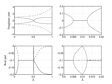
Figure 4: Imaginary parts (upper row) and real parts (lower row) of the eigenvalues in the linearized Holstein-Primakoff representation as a function of the coupling strength $\lambda$; for $\omega=\omega_{0}=1$ and $\kappa=0.2$. Solid (dashed) lines correspond to the photonic (atomic) branch. The right-hand column magnifies the view around the transition at $\lambda=\lambda_{c}=0.5099$; note the splitting (convergence) at $\lambda^{\prime}\simeq 0.5050$ and $\lambda^{\prime\prime}\simeq 0.5124$.

To complement the figure, in the range $0\leq\lambda\leq\kappa/2$, the eigenvalues are given by (with $\omega=\omega_{0}$)

$$\epsilon_{\rm ph}^{\pm} = -\kappa/2\pm i\sqrt{\omega_{0}^{2}-\kappa^{2}/4\pm\Lambda},$$ (35a)

$$\epsilon_{\rm at}^{\pm} = -\kappa/2\pm i\sqrt{\omega_{0}^{2}-\kappa^{2}/4\mp\Lambda},$$ (35b)

with

$$\Lambda=\sqrt{\omega_{0}^{2}(4\lambda^{2}-\kappa^{2})},$$ (36)

where both upper or lower signs are to be taken, while for $\kappa/2\leq\lambda\leq\lambda_{\rm c}$,

$$\epsilon_{\rm ph}^{\pm} = -\kappa/2\pm i\sqrt{\omega_{0}^{2}-\kappa^{2}/4-\Lambda},$$ (37a)

$$\epsilon_{\rm at}^{\pm} = -\kappa/2\pm i\sqrt{\omega_{0}^{2}-\kappa^{2}/4+\Lambda}.$$ (37b)

Thus we see that $\epsilon_{\rm ph}^{-}\rightarrow 0$, $\epsilon_{\rm ph}^{+}\rightarrow-\kappa$, and $\epsilon_{\rm at}^{\pm}\rightarrow-\kappa/2\pm i\sqrt{2\omega_{0}^{2}-\kappa^{2}/4}$ as the critical coupling is approached.

Above the critical point, similarly simple expressions cannot be found. We note, however, that for $\lambda>\lambda^{\prime\prime}$ the photonic branch eigenvalues take on nonzero imaginary parts once again, and for large $\lambda$ approach $-\kappa\pm i\omega_{0}$. The atomic branch eigenvalues approach $\pm i\omega_{0}/\tilde{\mu}$, with a rapidly decreasing real part that scales like $\tilde{\mu}^{4}=(\lambda_{\rm c}/\lambda)^{8}$.

IV.3 Quantum Langevin equations and input-output theory

The equations of motion of the previous sections concern the “internal” dynamics of the atom-cavity system. To probe this dynamics we consider measurements on the light leaving the system through the cavity output mirror. We make use of the standard input-output theory of open quantum-optical systems Collett84 ; Gardiner85 ; Walls94 ; Carmichael99 , which is nicely formulated in terms of quantum Langevin equations for system operators: for $\lambda<\lambda_{\rm c}$,

$$\dot{\hat{a}} = -i\left[\hat{a},\hat{H}^{(1)}\right]-\kappa\hat{a}+\sqrt{2\kappa}\,\hat{a}_{\rm in}(t),$$ (38a)

$$\dot{\hat{b}} = -i\left[\hat{b},\hat{H}^{(1)}\right],$$ (38b)

plus the adjoint equations, while for $\lambda>\lambda_{\rm c}$,

$$\dot{\hat{c}} = -i\left[\hat{c},\hat{H}^{(2)}\right]-\kappa\hat{c}+\sqrt{2\kappa}\,\hat{a}_{\rm in}(t),$$ (39a)

$$\dot{\hat{d}} = -i\left[\hat{d},\hat{H}^{(2)}\right],$$ (39b)

plus the adjoint equations. The operator $\hat{a}_{\rm in}(t)$ describes the quantum noise injected at the cavity input (Fig. 2) and satisfies the commutation relation

$$\left[\hat{a}_{\rm in}(t),\hat{a}_{\rm in}^{\dagger}(t^{\prime})\right]=\delta(t-t^{\prime}).$$ (40)

In addition, for vacuum or coherent state inputs, one has the correlations

$$\langle\hat{a}_{\rm in}(t),\hat{a}_{\rm in}^{\dagger}(t^{\prime})\rangle = \delta(t-t^{\prime}),$$ (41a)

$$\langle\hat{a}_{\rm in}^{\dagger}(t),\hat{a}_{\rm in}(t^{\prime})\rangle = \langle\hat{a}_{\rm in}(t),\hat{a}_{\rm in}(t^{\prime})\rangle=0,$$ (41b)

where $\langle\hat{A},\hat{B}\rangle\equiv\langle\hat{A}\hat{B}\rangle-\langle\hat{A}\rangle\langle\hat{B}\rangle$. The cavity output field, $\hat{a}_{\rm out}(t)$, is given in terms of the intracavity and cavity input fields as

$$\hat{a}_{\rm out}(t)=\sqrt{2\kappa}\,\hat{a}(t)-\hat{a}_{\rm in}(t),$$ (42)

from which one calculates the output field correlation functions and spectra.

The quantum Langevin equations are linear operator equations. For the purpose of computing spectra, they are conveniently solved in frequency space by introducing the Fourier transforms

$$\tilde{\cal O}(\nu) = \frac{1}{\sqrt{2\pi}}\int_{-\infty}^{\infty}e^{i\nu t}\hat{\cal O}(t)\,{\rm d}t,$$ (43a)

$$\tilde{\cal O}^{\dagger}(-\nu) = \frac{1}{\sqrt{2\pi}}\int_{-\infty}^{\infty}e^{i\nu t}\hat{\cal O}^{\dagger}(t)\,{\rm d}t,$$ (43b)

where $\hat{\cal O}$ denotes any one of the operators $\hat{a}$, $\hat{b}$, $\hat{c}$, $\hat{d}$, or $\hat{a}_{\rm in}$. In the resonant case, $\omega_{0}=\omega$, the solutions are: for $\lambda<\lambda_{\rm c}$,

$$\tilde{a}(\nu) = \sqrt{2\kappa}\,\frac{\left\{\left[\kappa-i(\nu+\omega_{0})\right]\left(\nu^{2}-\omega_{0}^{2}\right)-2i\omega_{0}\lambda^{2}\right\}\tilde{a}_{\rm in}(\nu)-2i\omega_{0}\lambda^{2}\tilde{a}_{\rm in}^{\dagger}(-\nu)}{\left[\kappa-i(\nu-\omega_{0})\right]\left[\kappa-i(\nu+\omega_{0})\right]\left(\nu^{2}-\omega_{0}^{2}\right)+4\omega_{0}^{2}\lambda^{2}},$$ (44a)

$$\tilde{b}(\nu) = \frac{\lambda}{\nu-\omega_{0}}\left[\tilde{a}(\nu)+\tilde{a}^{\dagger}(-\nu)\right],$$ (44b)

and for $\lambda>\lambda_{\rm c}$,

$$\tilde{c}(\nu) = \sqrt{2\kappa}\,\frac{\left\{\left[\kappa-i(\nu+\omega_{0})\right]\left(\nu^{2}-\omega_{0}^{2}/\tilde{\mu}^{2}\right)-2i\omega_{0}\lambda^{2}\tilde{\mu}\right\}\tilde{a}_{\rm in}(\nu)-2i\omega_{0}\lambda^{2}\tilde{\mu}\,\tilde{a}_{\rm in}^{\dagger}(-\nu)}{\left[\kappa-i(\nu-\omega_{0})\right]\left[\kappa-i(\nu+\omega_{0})\right]\left(\nu^{2}-\omega_{0}^{2}/\tilde{\mu}^{2}\right)+4\omega_{0}^{2}\lambda^{2}\tilde{\mu}},$$ (45a)

$$\tilde{d}(\nu) = \frac{\lambda\tilde{\mu}\sqrt{2/(1+\tilde{\mu})}}{\nu-\omega_{0}(1+\tilde{\mu})/(2\tilde{\mu})}\left[\tilde{c}(\nu)+\tilde{c}^{\dagger}(-\nu)\right].$$ (45b)

IV.4 Entanglement of the atoms and field

Quantum fluctuations in the linearized treatment are Gaussian, and the solutions to the quantum Langevin equations can be used to compute their covariances in the steady state. For example, the mean intracavity photon number for $\lambda<\lambda_{\rm c}$ is given by

$$\langle\hat{a}^{\dagger}\hat{a}\rangle_{\rm ss}=\frac{1}{2\pi}\int_{-\infty}^{\infty}\int_{-\infty}^{\infty}\langle\hat{a}^{\dagger}(\nu)\hat{a}(\nu^{\prime})\rangle\,{\rm d}\nu\,{\rm d}\nu^{\prime},$$ (46)

where we need the frequency-space equivalents of the input correlations (41a) and (41b), i.e.,

$$\langle\tilde{a}_{\rm in}(\nu),\tilde{a}_{\rm in}^{\dagger}(\nu^{\prime})\rangle = \delta(\nu-\nu^{\prime}),$$ (47a)

$$\langle\tilde{a}_{\rm in}^{\dagger}(\nu),\tilde{a}_{\rm in}(\nu^{\prime})\rangle = \langle\tilde{a}_{\rm in}(\nu),\tilde{a}_{\rm in}(\nu^{\prime})\rangle=0.$$ (47b)

The computed output photon flux from the cavity, $2\kappa\langle\hat{a}^{\dagger}\hat{a}\rangle_{\rm ss}$, is plotted for several different values of $\kappa$ in Fig. 5, illustrating a “smoothing-out” of the transition with increasing cavity linewidth. The mean excitation of the atomic mode, $\langle\hat{b}^{\dagger}\hat{b}\rangle_{\rm ss}$, shows similar behavior.

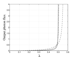
Figure 5: Output photon flux as a function of coupling strength; for $\omega=\omega_{0}=1$ and $\kappa=0.1$ (solid), $0.2$ (dashed), and $0.5$ (dot-dashed).

Of particular interest is the behavior of the bipartite quantum entanglement in the vicinity of the critical point Lambert04a ; Lambert05 ; Reslen05 ; Osterloh02 ; Osborne02 ; Vidal03 ; Vidal04 ; Wu04 ; Latorre05 . The cavity and atomic modes are natural choices for the entangled subsystems, and given that their fluctuations are described by a Gaussian continuous variable state, the criterion for inseparability can be formulated in terms of the variances of appropriate subsystem operators. In particular, we define the quadrature operators

$$\hat{X}_{a}^{\theta} = \frac{1}{2}\left(\hat{a}e^{-i\theta}+\hat{a}^{\dagger}e^{i\theta}\right),$$ (48a)

$$\hat{X}_{b}^{\phi} = \frac{1}{2}\left(\hat{b}e^{-i\phi}+\hat{b}^{\dagger}e^{i\phi}\right),$$ (48b)

with adjustable phases $\theta$ and $\phi$, and introduce the EPR (Einstein-Podolsky-Rosen) operators

$$\hat{u}=\hat{X}_{a}^{\theta}+\hat{X}_{b}^{\phi},\qquad\hat{v}=\hat{X}_{a}^{\theta+\pi/2}-\hat{X}_{b}^{\phi+\pi/2}.$$ (49)

Then a sufficient condition for the inseparability of the state below the critical point is (any $\theta$ and $\phi$) Duan00

$$\langle(\Delta\hat{u})^{2}\mkern 1.0mu\rangle+\langle(\Delta\hat{v})^{2}\mkern 1.0mu\rangle<1.$$ (50)

Alternatively, a stronger condition may be given in the modified form Giovannetti03

$$\langle(\Delta\hat{u})^{2}\mkern 1.0mu\rangle\langle(\Delta\hat{v})^{2}\mkern 1.0mu\rangle<\frac{1}{4}.$$ (51)

Above the critical point, similar definitions and conditions based on operators $\hat{c}$ and $\hat{d}$ hold. Here the EPR variance is associated with a quantum state “localized” about one of the two possible semiclassical steady states (23a)–(23c); within our linearized treatment transitions between these states are ignored.

The sum of EPR operator variances—inequality (50)—is plotted as a function of the coupling strength in Fig. 6. It approaches a cusp-like minimum at the critical coupling strength; thus, the entanglement here is maximum. The variance product—inequality (51)—exhibits similar behavior. These variances are measurable quantities. They offer a means of tracking entanglement across the phase transition. In fact, as we show in Sec. IV.5.4, variance-based entanglement measures can, under appropriate conditions, be deduced from measurements on the cavity output field alone.

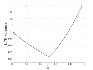
Figure 6: Sum of EPR operator variances as a function of coupling strength; for $\omega=\omega_{0}=1$, $\kappa=0.2$, $\theta=\tan^{-1}(\kappa/\omega)$, and $\phi=0$. The choice of $\theta$ minimizes the sum in the vicinity of the critical coupling strength, $\lambda=\lambda_{\rm c}\simeq 0.51$.

IV.5 Spectra of the cavity output field

Cavity output field spectra can be computed from the solutions to the Langevin equations (44a) and (45a), the correlations (47a) and (47b), and the input-output relations

$$\tilde{a}_{\rm out}(\nu)=\sqrt{2\kappa}\,\tilde{a}(\nu)-\tilde{a}_{\rm in}(\nu),$$ (52)

$\lambda<\lambda_{\rm c}$, and

$$\tilde{a}_{\rm out}(\nu)=\sqrt{2\kappa}\,\left[\tilde{c}(\nu)+\sqrt{2\pi}\,\alpha_{\rm ss}\delta(\nu)\right]-\tilde{a}_{\rm in}(\nu),$$ (53)

$\lambda>\lambda_{\rm c}$. We consider three standard spectra: (i) the fluorescence (or power) spectrum, which is proportional to the probability of detecting a photon of frequency $\nu$ at the cavity output, (ii) the probe transmission spectrum, the transmitted intensity as a function of frequency of a (weak) probe field applied at the cavity input, and (iii) homodyne spectra, which measure the quantum noise variances of output field quadrature amplitudes.

IV.5.1 Fluorescence spectrum

The fluorescence spectrum consists of a coherent part, representing the mean excitation of the intracavity field, the semiclassical solution $\alpha_{\rm ss}$, and an incoherent part which accounts for the quantum fluctuations. The latter is defined by

$$\langle\tilde{a}_{\rm out}^{\dagger}(\nu),\tilde{a}_{\rm out}(\nu^{\prime})\rangle=S(\nu)\delta(\nu-\nu^{\prime}).$$ (54)

It can also be expressed in terms of the steady state autocorrelation function of the intracavity field, with

$$S^{(1)}(\nu)=\int_{-\infty}^{\infty}e^{-i\nu\tau}\langle\hat{a}^{\dagger}(\tau),\hat{a}(0)\rangle_{\rm ss}{\rm d}\tau,$$ (55)

$\lambda<\lambda_{\rm c}$, and

$$S^{(2)}(\nu)=\int_{-\infty}^{\infty}e^{-i\nu\tau}\langle\hat{c}^{\dagger}(\tau),\hat{c}(0)\rangle_{\rm ss}{\rm d}\tau,$$ (56)

$\lambda>\lambda_{\rm c}$. Making use of solutions (44a) and (45a) for $\tilde{a}(\nu)$ and $\tilde{c}(\nu)$, and the input correlations (47a) and (47b), one finds

$$S^{(1,2)}(\nu)=\left|\frac{4\kappa\omega_{0}\lambda^{2}\tilde{\mu}^{(1,2)}}{\left[\kappa-i(\nu-\omega_{0})\right]\left[\kappa-i(\nu+\omega_{0})\right]\left[\nu^{2}-\omega_{0}^{2}/\left(\tilde{\mu}^{(1,2)}\right)^{2}\right]+4\omega_{0}^{2}\lambda^{2}\tilde{\mu}^{(1,2)}}\right|^{2},$$ (57)

with the definitions

$$\tilde{\mu}^{(1)}=1,\qquad\tilde{\mu}^{(2)}=\lambda_{\rm c}^{2}/\lambda^{2}.$$ (58)

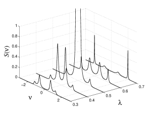
Figure 7: Incoherent part of the cavity fluorescence spectrum $S(\nu)$ for various values of coupling strength $\lambda$; for $\omega=\omega_{0}=1$ and $\kappa=0.2$ ($\lambda_{\rm c}\simeq 0.51$).

Sample spectra $S^{(1,2)}(\nu)$ are plotted in Fig. 7. The positions and widths of the spectral peaks are determined by the eigenvalues of the linearized dynamics discussed in Sec. IV.2.3. Thus, below the critical point the spectrum shows central and outer doublets associated with the photonic and atomic branch eigenvalues, respectively. The peaks of the photonic branch doublet merge as $\lambda\rightarrow\lambda_{\rm c}$, forming a single narrow peak at $\nu=0$; within the linearized treatment the intensity under this peak diverges at $\lambda=\lambda_{\rm c}$. Above the critical point a pair of doublets appears again. Far above the critical point the photonic branch peaks approach detunings determined by the cavity mode resonance frequency, $\nu\simeq\pm\omega=\pm 1$, and linewidths (FWHM) $2\kappa=0.4$. The atomic branch peaks move linearly apart, following the increasing Rabi frequency in the presence of the increasing mean intracavity field; they also become increasingly sharp.

Note that the symmetry of the spectra is ensured by energy conservation and the fact that, due to the symmetrical nature of the atom-cavity coupling, photon emissions from the cavity can be associated with transitions to either lower or higher internal energy states of the atom-cavity system.

IV.5.2 Probe transmission spectrum

One may also examine the system by driving the cavity mode with a (weak) laser field and measuring the intensity of the coherent transmission as a function of laser frequency. Such a measurement provides a rather direct probe of the energy level structure of the atom-cavity system; only when the laser frequency matches a system resonance would substantial transmission be expected.

Analytically, we treat the measurement by adding a driving term, ${\cal E}_{\rm p}e^{-i\nu_{\rm p}t}$, to the equations of motion for $\hat{a}$ and $\hat{c}$, where ${\cal E}_{\rm p}$ and $\nu_{\rm p}$ are the probe field amplitude and frequency. Solving the equations of motion in frequency space as before, the coherent amplitude in transmission follows straightforwardly from the coefficient of $\delta(\nu-\nu_{\rm p})$ in the solution for $\langle\tilde{a}_{\rm out}(\nu)\rangle$. The transmitted probe intensity is thus found to be

$$T^{(1,2)}(\nu_{\rm p})=\kappa^{2}\left|\frac{\left[\kappa-i(\nu_{\rm p}+\omega_{0})\right]\left[\nu_{\rm p}^{2}-\omega_{0}^{2}/\left(\tilde{\mu}^{(1,2)}\right)^{2}\right]-2i\omega_{0}\lambda^{2}\tilde{\mu}^{(1,2)}}{\left[\kappa-i(\nu_{\rm p}-\omega_{0})\right]\left[\kappa-i(\nu_{\rm p}+\omega_{0})\right]\left[\nu_{\rm p}^{2}-\omega_{0}^{2}/\left(\tilde{\mu}^{(1,2)}\right)^{2}\right]+4\omega_{0}^{2}\lambda^{2}\tilde{\mu}^{(1,2)}}\right|^{2},$$ (59)

with $\tilde{\mu}^{(1)}$ and $\tilde{\mu}^{(2)}$ defined by Eq. (58); the normalization is such that the spectrum is a Lorentzian of width $2\kappa$ and unit height when $\lambda$ is set to zero.

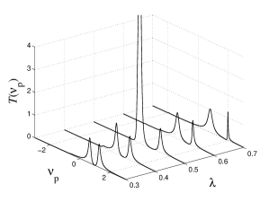
Figure 8: Probe transmission spectrum $T(\nu_{\rm p})$ for various values of the coupling strength $\lambda$; for $\omega=\omega_{0}=1$ and $\kappa=0.2$ ($\lambda_{\rm c}\simeq 0.51$).

A series of probe transmission spectra are plotted in Fig. 8, where we choose values of coupling strength to correspond to Fig. 7. The spectra contain two principal peaks, one associated with the photonic and one with the atomic branch. Their behavior as a function of $\lambda$ replicates the behavior displayed by the fluorescence.

IV.5.3 Homodyne spectra

Homodyne spectra measure the fluctuation variances in frequency space of the output field quadrature amplitudes. Quadrature operators are defined in time and frequency space, respectively, as

$$\hat{X}_{{\rm out},\theta} = \frac{1}{2}\left(\hat{a}_{\rm out}e^{-i\theta}+\hat{a}_{\rm out}^{\dagger}e^{i\theta}\right),$$ (60a)

$$\tilde{X}_{{\rm out},\theta}(\nu) = \frac{1}{2}\left[\tilde{a}_{\rm out}(\nu)e^{-i\theta}+\tilde{a}_{\rm out}^{\dagger}(-\nu)e^{i\theta}\right],$$ (60b)

where $$\theta S_{{\rm out},\theta}(\nu)$$ is the quadrature phase. The (normally-ordered) homodyne spectrum, , is defined by the variance Collett84 ; Walls94

$$\langle\mkern 2.0mu:\mkern-2.0mu\tilde{X}_{{\rm out},\theta}(\nu),\tilde{X}_{{\rm out},\theta}(\nu^{\prime})\mkern-2.0mu:\mkern 2.0mu\rangle=S_{{\rm out},\theta}(\nu)\,\delta(\nu+\nu^{\prime}),$$ (61)

which we compute from the input-output relation (42) and solutions (44a) and (45a) for the intracavity fields. Note that with the choice of normal ordering the vacuum noise level corresponds to $S_{{\rm out},\theta}(\nu)=0$, while perfect quantum noise reduction corresponds to $S_{{\rm out},\theta}(\nu)=-1/4$.

Numerical results for $\theta=0$ and $\theta=\pi/2$ are presented in Fig. 9. As the coupling strength approaches $\lambda_{\rm c}$, the phase transition is signaled by a divergence of the quadrature amplitude flutuations at $\nu=0$, similar to the behavior of the cavity fluorescence (Fig. 7). Nonetheless, there is an optimal $\theta$ at each $\lambda$, for which near-perfect noise reduction occurs in the $(\theta+\pi/2)$-quadrature at $\nu=0$. Figure 10 plots the optimal phase and corresponding minimum quadrature variance across the threshold region. As $\lambda\rightarrow\lambda_{\rm c}$, the optimal phase approaches $\theta_{\rm min}=\tan^{-1}(\kappa/\omega)+\pi/2$.

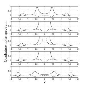
Figure 9: Quadrature noise spectra $S_{{\rm out},\theta}(\nu)$ with $\theta=0$ (solid) and $\theta=\pi/2$ (dashed); for $\omega=\omega_{0}=1$, $\kappa=0.2$ ($\lambda_{\rm c}\simeq 0.51$), and $\lambda=0.4,0.49,0.505,0.52,0.6$ (top to bottom).

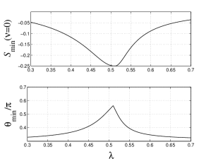
Figure 10: Optimal squeezing at $\nu=0$ as a function of $\lambda$ (top) and the quadrature phase angle at which the optimum occurs (bottom); for $\omega=\omega_{0}=1$ and $\kappa=0.2$ ($\lambda_{\rm c}\simeq 0.51$).

Well above the critical point the noise level returns to the vacuum noise level at all frequencies, except close to the atomic branch resonances at $\nu\simeq\pm\omega_{0}/\tilde{\mu}$. Here significant squeezing below the vacuum noise level is found for the $\theta=0$ quadrature amplitude, with corresponding amplification of the fluctuations at $\theta=\pi/2$. In fact, substantial squeezing of the atomic branch resonances occurs also for $\lambda<\lambda_{\rm c}$, as seen from Fig. 9. Although the bandwidth of this squeezing becomes increasingly narrow as $\lambda$ increases, the noise reduction on resonance actually approaches 100%.

IV.5.4 Output field squeezing and atom-field entanglement

For the parameter regime we have considered, the spectra presented exhibit distinct features that can be identified with either the “photonic” or “atomic” branches. The lower frequency peaks are associated with the photonic branch and the higher frequency peaks with the atomic branch. The corresponding photonic and atomic modes are formalized by a diagonalization of Hamiltonians (26) and (30) via Bogoliubov transformations, as shown in Emary03b and outlined in Appendix A. If these modes are well separated in frequency, and $\kappa$ is sufficiently small, then one can also associate with them what are essentially independent and uncorrelated output fields, $\hat{a}_{\rm out}^{\rm at}(t)$ and $\hat{a}_{\rm out}^{\rm ph}(t)$; hence, we can relate their quadrature variances to the quadrature variances of linear combinations of the “bare” internal atomic and cavity modes. In particular, in the normal phase, we find that the EPR variance of Eq. (50) (with $\phi=\theta$) is approximately given by (Appendix A)

$$\frac{2}{\kappa}\left(\langle\mkern 3.0mu:\mkern-2.0mu\hat{X}_{{\rm out},\theta}^{\rm at},\hat{X}_{{\rm out},\theta}^{\rm at}\mkern-2.0mu:\mkern 3.0mu\rangle+\langle\mkern 3.0mu:\mkern-2.0mu\hat{X}_{{\rm out},\theta+\pi/2}^{\rm ph},\hat{X}_{{\rm out},\theta+\pi/2}^{\rm ph}\mkern-2.0mu:\mkern 3.0mu\rangle\right)+1,$$ (62)

where the output field quadrature variances are calculated from integrals of the (normally-ordered) homodyne spectrum over appropriate frequency ranges, i.e.,

$$\langle\mkern 3.0mu:\mkern-2.0mu\hat{X}_{{\rm out},\theta+\pi/2}^{\rm ph},\hat{X}_{{\rm out},\theta+\pi/2}^{\rm ph}\mkern-2.0mu:\mkern 3.0mu\rangle = \frac{1}{2\pi}\int_{\{\nu_{\rm ph}\}}S_{{\rm out},\theta+\pi/2}(\nu)\,{\rm d}\nu,$$ (63a)

$$\langle\mkern 3.0mu:\mkern-2.0mu\hat{X}_{{\rm out},\theta}^{\rm at},\hat{X}_{{\rm out},\theta}^{\rm at}\mkern-2.0mu:\mkern 3.0mu\rangle = \frac{1}{2\pi}\int_{\{\nu_{\rm at}\}}S_{{\rm out},\theta}(\nu)\,{\rm d}\nu.$$ (63b)

If one then considers the homodyne spectra plotted for $$\lambda=0.4 0.49 S_{{\rm out},0}(\nu) S_{{\rm out},\pi/2}(\nu) \theta=0,\,\pi/2$$ and in Fig. 9, qualitatively, these expressions allow entanglement to be inferred from the fact that exhibits squeezing—i.e., is negative—on the atomic branch while exhibits squeezing on the photonic branch. Given the well-defined peaks and dips in the homodyne spectra around , we estimate (62) by

$$V_{\rm est}=\frac{2}{\kappa}\frac{1}{2\pi}\left\{\int_{S_{{\rm out},\theta}(\nu)<0}S_{{\rm out},\theta}(\nu)\,{\rm d}\nu+\int_{S_{{\rm out},\theta+\pi/2}(\nu)<0}S_{{\rm out},\theta+\pi/2}(\nu)\,{\rm d}\nu\right\}+1.$$ (64)

This quantity is plotted as a function of $\lambda$ in Fig. 11. For $\lambda<\lambda_{\rm c}$, it shows rather good agreement with the EPR variance plotted in Fig. 6; the agreement improves for decreasing values of the decay rate $\kappa$. Above threshold, on the other hand, $V_{\rm est}$ can only be regarded as a good measure of entanglement when $\lambda$ is quite close to $\lambda_{\rm c}$. In the superradiant phase, the relationships between output field and internal mode operators are more complicated [compare Eqs. (70a)–(71b) and (77a)–(81b], but entanglement measures based on output field quadrature variances can still be derived. The measures depend explicitly on $\lambda$, however, and cannot be directly related to the EPR variance of Eq. (50), as was possible for the normal phase. Nevertheless, they do display a drop-off in the degree of entanglement with increasing $\lambda$, consistent with that shown in Fig. 6.

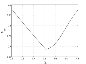
Figure 11: Estimate of the EPR variance, $V_{\rm est}$, as a function of coupling strength; for $\omega=\omega_{0}=1$, $\kappa=0.2$, and quadarture phase angle $\theta=\tan^{-1}(\kappa/\omega)\simeq 0.2$. The choice of $\theta$ minimizes $V_{\rm est}$ close to the threshold at $\lambda_{\rm c}\simeq 0.51$.

V Conclusion

In this paper we have proposed a scheme for the realization of an elementary atom-light interaction Hamiltonian – the so-called Dicke Model – which should enable the observation and detailed study of a quantum phase transition involving a collective atomic pseudo-spin and a single quantized mode of the electromagnetic field. While the optical cavity-QED system considered is necessarily dissipative, due to cavity loss, the dissipation is a positive feature providing a window through which one can monitor the system using standard quantum-optical measurement techniques. As we have demonstrated, fluorescence, probe transmission, and squeezing spectra all provide detailed information on the varying energy level structure of the Dicke Hamiltonian and exhibit striking behavior in the vicinity of the critical point.

We have focussed exclusively on the thermodynamic limit, with the number of atoms taken to infinity, where fluctuations may be treated using a bosonic approximation for the collective atomic spin and linearization about the semiclassical steady state. Finite-size systems are a natural consideration, both theoretically and experimentally, and are of interest for examining scaling properties and deviations from the linearized model. Indeed, in a regime of strong-coupling cavity QED (see, for example, McKeever03 ; Sauer04 ; Maunz05 ) it could be possible to realize the critical regime of the Dicke Model with just a few atoms. In such a case, issues of quantum measurement (e.g., measurement backaction) arise, providing a further interesting avenue of investigation.

Finite-size systems and a full treatment of the Dicke model without linearization are also of importance for studying the role of quantum entanglement in the vicinity of the phase transition. In the present paper we touched only briefly on this subject, demonstrating that variance-based measures of atom-field entanglement can in principle be determined from homodyne spectra of the cavity output field, thus enabling entanglement to be “monitored”. The proposed system clearly offers further exciting prospects for the study of entanglement in a quantum critical system. For example, with additional light fields (possibly including other cavity modes) one could envisage making independent measurements on the atomic ensemble to complement those made on the cavity field, enabling the explicit determination of correlations and entanglement measures such as the EPR variance. Separately addressable atomic sub-ensembles coupled to the same quantized cavity mode would also allow the measurement of entanglement between different “blocks” of spins Latorre05 .

Appendix A Normal modes and entanglement criteria

A.1 Normal phase

The normal-phase Hamiltonian (26) can be diagonalised in the form (omitting constant terms)

$$\hat{H}^{(1)}=\omega_{\rm ph}^{(1)}(\lambda)\hat{A}^{\dagger}\hat{A}+\omega_{\rm at}^{(1)}(\lambda)\hat{B}^{\dagger}\hat{B},$$ (65)

where $\omega_{\rm ph}^{(1)}(\lambda)$ and $\omega_{\rm at}^{(1)}(\lambda)$ are the normal mode frequencies, with respective normal mode operators Emary03b

$$\hat{A} = \frac{1}{2}\left(2\omega_{0}\omega_{\rm ph}^{(1)}\right)^{-1/2}\left[(\omega_{\rm ph}^{(1)}-\omega_{0})(\hat{a}^{\dagger}-\hat{b}^{\dagger})+(\omega_{\rm ph}^{(1)}+\omega_{0})(\hat{a}-\hat{b})\right],$$ (66a)

$$\hat{B} = \frac{1}{2}\left(2\omega_{0}\omega_{\rm at}^{(1)}\right)^{-1/2}\left[(\omega_{\rm at}^{(1)}-\omega_{0})(\hat{a}^{\dagger}+\hat{b}^{\dagger})+(\omega_{\rm at}^{(1)}+\omega_{0})(\hat{a}+\hat{b})\right],$$ (66b)

where $$\omega=\omega_{0} \hat{a}$$ has been assumed. The inverse relationship for the cavity mode operator is

$$\hat{a}=\frac{1}{2}\left\{\left(2\omega_{0}\omega_{\rm ph}^{(1)}\right)^{-1/2}\left[(\omega_{0}-\omega_{\rm ph}^{(1)})\hat{A}^{\dagger}+(\omega_{0}+\omega_{\rm ph}^{(1)})\hat{A}\right]+\left(2\omega_{0}\omega_{\rm at}^{(1)}\right)^{-1/2}\left[(\omega_{0}-\omega_{\rm at}^{(1)})\hat{B}^{\dagger}+(\omega_{0}+\omega_{\rm at}^{(1)})\hat{B}\right]\right\}.$$ (67)

If the normal modes are well separated in frequency with linewidths much smaller than their separation, within the bandwidth of the photonic mode the cavity mode contribution to the output field [Eq. (42)] may be written as

$$\hat{a}\simeq\frac{1}{2}\left(2\omega_{0}\omega_{\rm ph}^{(1)}\right)^{-1/2}\left[(\omega_{0}-\omega_{\rm ph}^{(1)})\hat{A}^{\dagger}+(\omega_{0}+\omega_{\rm ph}^{(1)})\hat{A}\right],$$ (68)

and within the bandwidth of the atomic mode as

$$\hat{a}\simeq\frac{1}{2}\left(2\omega_{0}\omega_{\rm at}^{(1)}\right)^{-1/2}\left[(\omega_{0}-\omega_{\rm at}^{(1)})\hat{B}^{\dagger}+(\omega_{0}+\omega_{\rm at}^{(1)})\hat{B}\right].$$ (69)

Using these approximations, the input-output relation (42), and Eqs. (66a) and (66b), one may derive approximate expressions for the output field quadrature operators in the specified frequency regions in terms of “bare” cavity and atomic mode operators:

$$\hat{X}_{{\rm out},\theta}^{\rm ph} \simeq \sqrt{2\kappa}\mkern 3.0mu(\hat{X}_{a}^{\theta}-\hat{X}_{b}^{\theta})/2-\hat{X}_{{\rm in},\theta}^{\rm ph},$$ (70a)

$$\hat{X}_{{\rm out},\theta}^{\rm at} \simeq \sqrt{2\kappa}\mkern 3.0mu(\hat{X}_{a}^{\theta}+\hat{X}_{b}^{\theta})/2-\hat{X}_{{\rm in},\theta}^{\rm at}.$$ (70b)

It follows that, in the normal phase, the normally-ordered output field variances can be directly related to the internal mode EPR variances Collett84 :

$$\langle\mkern 2.0mu:\!\hat{X}_{{\rm out},\theta}^{\rm ph},\hat{X}_{{\rm out},\theta}^{\rm ph}\!:\mkern 2.0mu\rangle \simeq \frac{\kappa}{2}\langle\mkern 2.0mu:\!\hat{X}_{a}^{\theta}-\hat{X}_{b}^{\theta},\hat{X}_{a}^{\theta}-\hat{X}_{b}^{\theta}\!:\mkern 2.0mu\rangle,$$ (71a)

$$\langle\mkern 2.0mu:\!\hat{X}_{{\rm out},\theta}^{\rm at},\hat{X}_{{\rm out},\theta}^{\rm at}\!:\mkern 2.0mu\rangle \simeq \frac{\kappa}{2}\langle\mkern 2.0mu:\!\hat{X}_{a}^{\theta}+\hat{X}_{b}^{\theta},\hat{X}_{a}^{\theta}+\hat{X}_{b}^{\theta}\!:\mkern 2.0mu\rangle,\mkern 30.0mu$$ (71b)

where a vacuum field input has been assumed. Then, adopting the entanglement criterion from Duan00 , entanglement between the cavity and atomic modes can be inferred whenever the inequality

$$\langle\mkern 3.0mu:\mkern-2.0mu\hat{X}_{{\rm out},\theta}^{\rm at},\hat{X}_{{\rm out},\theta}^{\rm at}\mkern-2.0mu:\mkern 3.0mu\rangle+\langle\mkern 3.0mu:\mkern-2.0mu\hat{X}_{{\rm out},\theta+\pi/2}^{\rm ph},\hat{X}_{{\rm out},\theta+\pi/2}^{\rm ph}\mkern-2.0mu:\mkern 3.0mu\rangle<0$$ (72)

is satisfied.

A.2 Superradiant phase

The superradiant-phase Hamiltonian (30) can be diagonalised in similar fashion in the form (omitting constant terms)

$$\hat{H}^{(2)}=\omega_{\rm ph}^{(2)}(\lambda)\hat{C}^{\dagger}\hat{C}+\omega_{\rm at}^{(2)}(\lambda)\hat{D}^{\dagger}\hat{D},$$ (73)

where $\omega_{\rm ph}^{(2)}$ and $\omega_{\rm at}^{(2)}$ are the above threshold normal mode frequencies (for linearization around either of the above threshold steady states), and the respective normal mode operators are given by the somewhat more complicated expressions Emary03b

$$\hat{C} = \frac{1}{2}\left\{\frac{\cos\gamma^{(2)}}{\sqrt{\omega_{0}\omega_{\rm ph}^{(2)}}}\left[(\omega_{\rm ph}^{(2)}-\omega_{0})\hat{c}^{\dagger}+(\omega_{\rm ph}^{(2)}+\omega_{0})\hat{c}\right]-\frac{\sin\gamma^{(2)}}{\sqrt{\tilde{\omega}_{0}\omega_{\rm ph}^{(2)}}}\left[(\omega_{\rm ph}^{(2)}-\tilde{\omega}_{0})\hat{d}^{\dagger}+(\omega_{\rm ph}^{(2)}+\tilde{\omega}_{0})\hat{d}\right]\right\},$$ (74a)

$$\hat{D} = \frac{1}{2}\left\{\frac{\sin\gamma^{(2)}}{\sqrt{\omega_{0}\omega_{\rm at}^{(2)}}}\left[(\omega_{\rm at}^{(2)}-\omega_{0})\hat{c}^{\dagger}+(\omega_{\rm at}^{(2)}+\omega_{0})\hat{c}\right]+\frac{\cos\gamma^{(2)}}{\sqrt{\tilde{\omega}_{0}\omega_{\rm at}^{(2)}}}\left[(\omega_{\rm at}^{(2)}-\tilde{\omega}_{0})\hat{d}^{\dagger}+(\omega_{\rm at}^{(2)}+\tilde{\omega}_{0})\hat{d}\right]\right\},$$ (74b)

with

$$\tan(2\gamma^{(2)})=2\tilde{\mu}^{2}(1-\tilde{\mu}^{2})^{-1},$$ (75)

$$\tilde{\omega}_{0}=\omega_{0}(1+\tilde{\mu}^{-1})/2,$$ (76)

where, once again, the resonance condition $\omega=\omega_{0}$ has been assumed. These expressions do not allow for as simple a relationship between output field and internal mode quadrature variances to be written down. Nevertheless, following the same arguments as before, one can write

$$\hat{X}_{{\rm out},\theta}^{\rm ph} \simeq \sqrt{2\kappa}\mkern 3.0mu\hat{X}_{cd}^{\theta}-\hat{X}_{{\rm in},\theta}^{\rm ph},$$ (77a)

$$\hat{X}_{{\rm out},\theta}^{\rm at} \simeq \sqrt{2\kappa}\mkern 3.0mu\hat{Y}_{cd}^{\theta}-\hat{X}_{{\rm in},\theta}^{\rm at},$$ (77b)

where

$$\hat{X}_{cd}^{\theta} = \cos^{2}(\gamma^{(2)})\hat{X}_{c}^{\theta}-\cos(\gamma^{(2)})\sin(\gamma^{(2)})\mkern-2.0mu\left[\cos\theta\sqrt{\frac{\omega_{0}}{\tilde{\omega}_{0}}}\mkern 3.0mu\hat{X}_{d}^{\theta=0}+\sin\theta\sqrt{\frac{\tilde{\omega}_{0}}{\omega_{0}}}\mkern 3.0mu\hat{X}_{d}^{\theta=\pi/2}\right],$$ (78a)

$$\hat{Y}_{cd}^{\theta} = \sin^{2}(\gamma^{(2)})\hat{X}_{c}^{\theta}+\cos(\gamma^{(2)})\sin(\gamma^{(2)})\mkern-2.0mu\left[\cos\theta\sqrt{\frac{\omega_{0}}{\tilde{\omega}_{0}}}\mkern 3.0mu\hat{X}_{d}^{\theta=0}+\sin\theta\sqrt{\frac{\tilde{\omega}_{0}}{\omega_{0}}}\mkern 3.0mu\hat{X}_{d}^{\theta=\pi/2}\right].$$ (78b)

For these more complicated linear superpositions of the internal mode operators it is still possible to derive inseparability criteria based on their variances. In particular, following Giovannetti03 one can show that a sufficient condition for the inseparability of the system state is given by

$$V_{1}\equiv\frac{\left\langle(\Delta\hat{X}_{cd}^{\theta+\pi/2})^{2}\right\rangle+\left\langle(\Delta\hat{Y}_{cd}^{\theta})^{2}\right\rangle}{\cos^{2}(\gamma^{(2)})\sin^{2}(\gamma^{(2)})}<1,$$ (79)

or in stronger form

$$V_{2}\equiv\frac{\left\langle(\Delta\hat{X}_{cd}^{\theta+\pi/2})^{2}\right\rangle\left\langle(\Delta\hat{Y}_{cd}^{\theta})^{2}\right\rangle}{\frac{1}{4}\cos^{4}(\gamma^{(2)})\sin^{4}(\gamma^{(2)})}<1.$$ (80)

The required variances can be deduced from the (normally-ordered) photonic and atomic output field quadrature variances by inverting the relations

$$\langle\mkern 3.0mu:\hat{X}_{{\rm out},\theta+\pi/2}^{\rm ph},\hat{X}_{{\rm out},\theta+\pi/2}^{\rm ph}:\mkern 3.0mu\rangle\simeq 2\kappa\left\{\mkern-2.0mu\left\langle(\Delta\hat{X}_{cd}^{\theta+\pi/2})^{2}\right\rangle-\frac{1}{4}\left[\cos^{4}(\gamma^{(2)})+\cos^{2}(\gamma^{(2)})\sin^{2}(\gamma^{(2)})\mkern-2.0mu\left(\frac{\omega_{0}}{\tilde{\omega}_{0}}\sin^{2}\theta+\frac{\tilde{\omega}_{0}}{\omega_{0}}\cos^{2}\theta\right)\right]\mkern-2.0mu\right\},$$ (81a)

and

$$\langle\mkern 3.0mu:\hat{X}_{{\rm out},\theta}^{\rm at},\hat{X}_{{\rm out},\theta}^{\rm at}:\mkern 3.0mu\rangle\simeq 2\kappa\left\{\mkern-2.0mu\left\langle(\Delta\hat{Y}_{cd}^{\theta})^{2}\right\rangle-\frac{1}{4}\left[\sin^{4}(\gamma^{(2)})+\cos^{2}(\gamma^{(2)})\sin^{2}(\gamma^{(2)})\mkern-2.0mu\left(\frac{\omega_{0}}{\tilde{\omega}_{0}}\cos^{2}\theta+\frac{\tilde{\omega}_{0}}{\omega_{0}}\sin^{2}\theta\right)\right]\mkern-2.0mu\right\}.$$ (81b)

Numerical examples of $$V_{1} V_{2} \lambda V_{1} V_{2} \lambda$$ and versus are shown in Fig. 12. The output field quadrature variances used were computed via numerical integration of the homodyne spectra from Section IV.E.4. The computed and display a decay in the degree of entanglement with increasing , consistent with the internal mode EPR variance of Fig. 6.

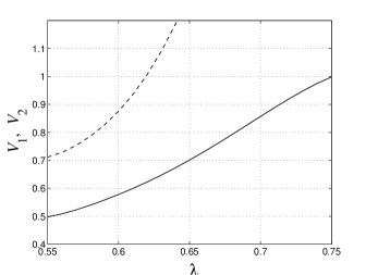
Figure 12: Entanglement measures $V_{1}$ (dashed) and $V_{2}$ (solid) versus coupling strength; for $\omega=\omega_{0}=1$, $\kappa=0.2$, and $\theta=0$.

References

- (1) R. H. Dicke, Phys. Rev. 93, 99 (1954).
- (2) K. Hepp and E. H. Lieb, Ann. Phys. (N.Y.) 76, 360 (1973).
- (3) K. Hepp and E. H. Lieb, Phys. Rev. A 8, 2517 (1973).
- (4) Y. K. Wang and F. T. Hioe, Phys. Rev. A 7, 831 (1973).
- (5) F.T. Hioe, Phys. Rev. A 8, 1440 (1973).
- (6) H. J. Carmichael, C. W. Gardiner, and D. F. Walls, Phys. Lett. A 46, 47 (1973).
- (7) G. Cromer Duncan, Phys. Rev. A 9, 418 (1974).
- (8) C. Emary and T. Brandes, Phys. Rev. Lett. 90, 044101 (2003).
- (9) C. Emary and T. Brandes, Phys. Rev. E 67, 066203 (2003).
- (10) N. Lambert, C. Emary, and T. Brandes, Phys. Rev. Lett. 92, 073602 (2004).
- (11) N. Lambert, C. Emary, and T. Brandes, Phys. Rev. A 71, 053804 (2005).
- (12) J. Reslen, L. Quiroga, and N. F. Johnson, Europhys. Lett. 69, 8 (2005).
- (13) T. Wilk et al., quant-ph/0603083. Note that these authors employ a scheme in which the two Raman channels involve different, circularly-polarized cavity modes.
- (14) D. Kruse et al., Phys. Rev. A 67, 051802(R) (2003).
- (15) B. Nagorny et al., Phys. Rev. A 67, 031401(R) (2003).
- (16) T. Holstein and H. Primakoff, Phys. Rev. 58, 1098 (1940).
- (17) E. Ressayre and A. Tallet, Phys. Rev. A 11, 981 (1975).
- (18) M. J. Collett and C. W. Gardiner, Phys. Rev. A 30, 1386 (1984).
- (19) C. W. Gardiner and M. J. Collett, Phys. Rev. A 31, 3761 (1985).
- (20) D. F. Walls and G. J. Milburn, Quantum Optics (Springer-Verlag, Berlin, 1994).
- (21) H. J. Carmichael, Statistical Methods in Quantum Optics: Master Equations and Fokker-Planck Equations (Springer-Verlag, Berlin, 1999).
- (22) A. Osterloh, L. Amico, G. Falci, and R. Fazio, Nature (London) 416, 608 (2002).
- (23) T. J. Osborne and M. A. Nielsen, Phys. Rev. A, 66, 032110, (2002).
- (24) G. Vidal, J. I. Latorre, E. Rico, and A. Kitaev, Phys. Rev. Lett. 90, 227902 (2003).
- (25) J. Vidal, G. Palacios, and R. Mosseri, Phys. Rev. A 69, 022107 (2004).
- (26) L.-A. Wu, M. S. Sarandy, and D. A. Lidar, Phys. Rev. Lett. 93, 250404 (2004).
- (27) J. I. Latorre, R. Orús, E. Rico, and J. Vidal, Phys. Rev. A 71, 064101 (2005).
- (28) L.-M. Duan, G. Giedke, J. I. Cirac, and P. Zoller, Phys. Rev. Lett. 84, 2722 (2000).
- (29) V. Giovannetti, S. Mancini, D. Vitali, and P. Tombesi, Phys. Rev. A 67, 022320 (2003).
- (30) J. McKeever et al., Phys. Rev. Lett. 90, 133602 (2003).
- (31) J. A. Sauer et al., Phys. Rev. A 69, 051804(R) (2004).
- (32) P. Maunz et al., Phys. Rev. Lett. 94, 033002 (2005).