Decoherence and Recoherence in a Vibrating RF SQUID

Abstract

We study an RF SQUID, in which a section of the loop is a freely suspended beam that is allowed to oscillate mechanically. The coupling between the RF SQUID and the mechanical resonator originates from the dependence of the total magnetic flux threading the loop on the displacement of the resonator. Motion of the latter affects the visibility of Rabi oscillations between the two lowest energy states of the RF SQUID. We address the feasibility of experimental observation of decoherence and recoherence, namely decay and rise of the visibility, in such a system.

I Introduction

Decoherence occurs when a quantum system is coupled to a noisy environment at a finite temperature. Decoherence is commonly quantified by a visibility factor, which characterizes the relative amplitude of a measured interference signal. In many cases the main contribution to decoherence originates from the many degrees of freedom of the environment, which all have a similar coupling strength to the interfering degree of freedom of the quantum system. In such a case the visibility factor is expected to decay monotonically as a function of time (typically, the decay is exponential). On the other hand, when only a few degrees of freedom in the environment significantly contribute, the time dependence of the visibility factor is not necessarily monotonic. Recoherence occurs when the visibility factor increases with time. Experimental demonstration of this phenomenon is important since it may provide a crucial test to the theory of quantum measurement Leggett (2002); Leggett and Garg (1985). Decoherence and recoherence were recently discussed theoretically in Refs. Armour and Blencowe (2001); Bose et al. (1997); Mancini et al. (1997); Marshall et al. (2003); Bernad et al. (2006); Armour et al. (2002); Cleland and Geller (2004). The interfering quantum system in Ref. Armour and Blencowe (2001) was a single level quantum dot, in Refs. Bose et al. (1997); Mancini et al. (1997); Marshall et al. (2003); Bernad et al. (2006) it was an optical mode in a cavity, and in Refs. Armour et al. (2002); Cleland and Geller (2004) a superconducting charge (Cooper-pair box) and phase Josephson qubit, respectively. In all these cases, the interfering quantum system is coupled to a vibrating mode of a mechanical resonator (typically the lowest, fundamental mode). Recoherence can occur in such systems provided that the coupling between the interfering quantum system and the mode of the mechanical resonator is made sufficiently strong, whereas the coupling to other degrees of freedom in the environment is sufficiently weak. Satisfying this condition experimentally when the interfering degree of freedom is a single electron, as in the Ref. Armour and Blencowe (2001), or a single photon, as in Refs. Bose et al. (1997); Mancini et al. (1997); Marshall et al. (2003); Bernad et al. (2006), turns out to be very difficult.

In the present paper we study an alternative configuration consisting of an RF superconducting quantum interference device (SQUID) integrated with a mechanical resonator in the shape of a doubly clamped beam. The dependence of the total magnetic flux threading the loop on the beam’s displacement leads to a coupling between the RF SQUID and the mechanical resonator. We study the effect of such a coupling on the visibility of Rabi oscillations between the two lowest energy states of the RF SQUID, and discuss the required conditions for experimental observation of decoherence and recoherence originating from the coupling to the mechanical resonator.

The paper is organized as follows. The Hamiltonian for the closed system is obtained in section II. An adiabatic approximation is employed in section III to simplify the equations of motion of the system by considering the mechanical motion as slow in comparison with the faster dynamics of the RF SQUID. Further simplification is achieved in section IV by taking into account only the two lowest energy levels of the RF SQUID. In section V we calculate the effect of the mechanical resonator on the visibility of Rabi oscillations between these two energy levels. Corrections due to finite temperature and mechanical damping are considered in sections VI and VII respectively. The validity of the adiabatic approximation is examined in section VIII. A numerical example is given in section IX and discussion and conclusions are given in section X.

Similar systems consisting of a SQUID integrated with a nanomechanical resonator have been recently studied theoretically. Zhou and Mizel have shown that nonlinear coupling between a DC SQUID and a mechanical resonator can be employed for producing squeezed states of the mechanical resonator Zhou and Mizel (2006). More recently, Xue et al. have shown that a flux qubit integrated with a nanomechanical resonator can form a cavity quantum electrodynamics system in the strong coupling region Xue et al. (2006).

II Hamiltonian of the Closed System

Consider the RF SQUID shown in the inset of Fig. 1, in which a section of the loop is freely suspended and allowed to oscillate mechanically. We assume the case where the fundamental mechanical mode vibrates in the plane of the loop and denote the amplitude of this flexural mode as $x$. Let $m$ be the effective mass of the fundamental mode, and $\omega_{0}$ its angular frequency. A magnetic field is applied perpendicularly to the plane of the loop. Let $\Phi_{e}$ be the externally applied flux for the case $x=0$, and $B$ is the component of the magnetic field normal to the plane of the loop at the location of the doubly clamped beam (it is assumed that $B$ is constant in the region where the beam oscillates). The total magnetic flux $\Phi$ threading the loop is given by

$$\Phi=\Phi_{e}+Blx+LI\ ,$$ (1)

where $L$ is the self inductance of the loop, and $l$ is an effective length of the beam. The contribution of other mechanical modes of the beam to $\Phi$ is assumed to be negligibly small.

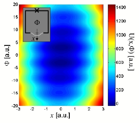
Figure 1: (Color online) The potential $U\left(x,\Phi\right)$ for the case $\Phi_{e}=\Phi_{0}/2$ and $\beta_{L}=20$. The inset schematically shows the device.

A Josephson junction (JJ) having a critical current $I_{c}$ and capacitance $C$ is integrated into the loop. We first consider the dynamics of the closed system consisting of the RF SQUID with the integrated doubly clamped beam. The effect of damping due to coupling to other degrees of freedom in the environment will be discussed later.

II.1 Lagrangian

The Lagrangian of the closed system is a function of the position $x$, flux $\Phi$ and their time derivatives (denoted by overdot):

$$\mathcal{L}=\frac{1}{2}m\dot{x}^{2}+\frac{C\dot{\Phi}^{2}}{2}-U\left(x,\Phi\right)\ ,$$ (2)

where the potential energy $U$ is given by

$$U=\frac{m\omega_{0}^{2}x^{2}}{2}+\frac{\left(\Phi-\Phi_{e}-Blx\right)^{2}}{2L}-\frac{\Phi_{0}I_{c}\cos\left(\frac{2\pi\Phi}{\Phi_{0}}\right)}{2\pi}\ ,$$ (3)

and $\Phi_{0}=h/2e$ is the flux quantum (see Fig. 1). The resulting Euler - Lagrange equations are

$$m\ddot{x}+m\omega_{0}^{2}x-\frac{Bl}{L}\left(\Phi-\Phi_{e}-Blx\right)=0\ ,$$ (4)

$$C\ddot{\Phi}+\frac{\Phi-\Phi_{e}-Blx}{L}+I_{c}\sin\left(\frac{2\pi\Phi}{\Phi_{0}}\right)=0\ .$$ (5)

Note that the gauge invariant phase across the Josephson junction $\gamma_{J}$ is given by

$$\gamma_{J}=2\pi n-\frac{2\pi\Phi}{\Phi_{0}}\ ,$$ (6)

where $n$ is integer. By using this and Eq. (1) the equations of motion can be rewritten as

$$m\ddot{x}+m\omega_{0}^{2}x-BlI=0\ ,$$ (7)

$$I_{c}\sin\gamma_{J}+C\frac{\Phi_{0}}{2\pi}\ddot{\gamma}_{J}=I\ .$$ (8)

The interpretation of these equations is straightforward. Eq. (7) expresses Newton’s 2nd law where the force is composed of the restoring mechanical force and the Lorentz force acting on the movable beam.  Whereas Eq. (8) states that the circulating current $I$ equals the sum of the current $I_{c}\sin\gamma_{J}$ through the JJ and the current $C\dot{V}$ through the capacitor, where the voltage $V$ is given by the second Josephson equation $V=\left(\Phi_{0}/2\pi\right)\dot{\gamma}_{J}$.

II.2 Hamiltonian

The variables canonically conjugate to $x$ and $\Phi$ are $p=\partial\mathcal{L}/\partial\dot{x}=m\dot{x}$ and $Q=\partial\mathcal{L}/\partial\dot{\Phi}=C\dot{\Phi}$ respectively. The Hamiltonian is given by

$$\mathcal{H} =\frac{p^{2}}{2m}+\frac{Q^{2}}{2C}+U\left(x,\Phi\right)\ .$$

(9)

Quantization is achieved by regarding the variables $x$, $p$, $\Phi$ and $Q$ as Hermitian operators satisfying the following commutation relations $\left[x,p\right]=\left[\Phi,Q\right]=i\hbar$ and $\left[x,\Phi\right]=\left[x,Q\right]=\left[p,\Phi\right]=\left[p,Q\right]=0$.

III Adiabatic Case

The Hamiltonian (9) can be written as $\mathcal{H}=\mathcal{H}_{0}+\mathcal{H}_{1}$, where

$$\mathcal{H}_{0}=\frac{p^{2}}{2m}+\frac{1}{2}m\omega_{0}^{2}x^{2}\ ,$$ (10)

$$\mathcal{H}_{1}=\frac{Q^{2}}{2C}+u\left(x,\Phi\right)\ .$$ (11)

Using the notation $U_{0}=\Phi_{0}^{2}/8\pi^{2}L$, $x_{\phi}=\Phi_{0}/Bl$, and $\beta_{L}=2\pi LI_{c}/\Phi_{0}$, the term $u$ can be written as

$$u=U_{0}\left[4\pi^{2}\left(\frac{\Phi-\Phi_{e}}{\Phi_{0}}-\frac{x}{x_{\phi}}\right)^{2}-2\beta_{L}\cos\left(\frac{2\pi\Phi}{\Phi_{0}}\right)\right]\ .$$ (12)

As a basis for expanding the general state of the system we use the solutions of the following Schrödinger equation

$$\mathcal{H}_{1}\left|n\left(x\right)\right\rangle=\varepsilon_{n}\left(x\right)\left|n\left(x\right)\right\rangle\ ,$$ (13)

where $x$ is treated here as a parameter (rather than a degree of freedom). The local eigenvectors are assumed to be orthonormal

$$\left\langle m\left(x\right)|n\left(x\right)\right\rangle=\delta_{nm}\ .$$ (14)

The wavefunctions associated with the local eigenstates

$$\varphi_{n,x}\left(\Phi^{\prime}\right)=\left\langle\Phi^{\prime}|n\left(x\right)\right\rangle\ ,$$ (15)

are the solutions of the Schrödinger equation

$$\left[-\frac{\hbar^{2}}{2C}\frac{\partial^{2}}{\partial\Phi^{2}}+u\left(\Phi;x\right)\right]\varphi_{n,x}=\varepsilon_{n}\left(x\right)\varphi_{n,x}\ .$$ (16)

The total wave function is expanded as

$$\psi\left(x,\Phi,t\right)=\sum_{n}\xi_{n}\left(x,t\right)\left|n\left(x\right)\right\rangle\ .$$ (17)

In the adiabatic approximation Moody et al. (1989) the time evolution of the coefficients $\xi_{n}$ is governed by the following set of decoupled equations of motion

$$\left[\frac{p^{2}}{2m}+V_{m}\left(x\right)\right]\xi_{m}=i\hbar\dot{\xi}_{m}\ ,$$ (18)

where the adiabatic potentials $V_{m}\left(x\right)$ are given by

$$V_{m}\left(x\right)=\frac{1}{2}m\omega_{0}^{2}x^{2}+\varepsilon_{m}\left(x\right)\ .$$ (19)

The validity of the adiabatic approximation will be discussed in section VIII below.

To numerically evaluate the eigenvalues $\varepsilon_{m}\left(x\right)$, it is convenient to introduce the dimensionless variables $2\pi\Phi/\Phi_{0}=\pi+\phi$, $2\pi\Phi_{e}/\Phi_{0}=\pi+\phi_{e}$, $2\pi x/x_{\phi}=\phi_{x}$. Using this notation the Schrödinger equation (16) can be rewritten as

$$\left(-\beta_{C}\frac{\partial^{2}}{\partial\phi^{2}}+\frac{u}{U_{0}}\right)\varphi_{n,x}=\lambda_{n,x}\varphi_{n,x}\ ,$$ (20)

where $\beta_{C}=2e^{2}/CU_{0}$,$\lambda_{n,x}=\varepsilon_{n}\left(x\right)/U_{0}$, and

$$\frac{u}{U_{0}}=\left(\phi-\phi_{e}-\phi_{x}\right)^{2}+2\beta_{L}\cos\phi\ .$$ (21)

IV Two-Level Approximation

Consider the case where $\left|\phi_{e}\right|\ll 1$ (namely, $\Phi_{e}\simeq\Phi_{0}/2$), $\left|\phi_{x}\right|\ll 1,$ and $\beta_{L}>1$. In this case the local potential $u\left(\phi\right)$ given by Eq. (21) contains two wells separated by a barrier near $\phi=0$. At low temperatures only the two lowest energy levels contribute. In this limit the local Hamiltonian $\mathcal{H}_{1}$ can be expressed in the basis of the states $\left|\curvearrowleft\right\rangle$ and $\left|\curvearrowright\right\rangle$, representing localized states in the left and right well respectively having opposite circulating currents. In this basis, $\mathcal{H}_{1}$ is represented by the $2\times 2$ matrix

$$\mathcal{H}_{1}=\left(\begin{array}[c]{cc}\eta\left(\phi_{e}+\phi_{x}\right)&\Delta\\ \Delta&-\eta\left(\phi_{e}+\phi_{x}\right)\end{array}\right)\ .$$ (22)

The real parameters $\eta$ and $\Delta$ can be determined by solving numerically the Schrödinger equation (20).

Using the notation

$$\tan\theta=\frac{\Delta}{\eta\left(\phi_{e}+\phi_{x}\right)}\ ,$$ (23)

$\mathcal{H}_{1}$ can be rewritten as

$$\mathcal{H}_{1}=\sqrt{\eta^{2}\left(\phi_{e}+\phi_{x}\right)^{2}+\Delta^{2}}\left(\begin{array}[c]{cc}\cos\theta&\sin\theta\\ \sin\theta&-\cos\theta\end{array}\right)\ .$$ (24)

The eigenvectors and eigenenergies are denoted as

$$\mathcal{H}_{1}\left|\pm\right\rangle=\varepsilon_{\pm}\left|\pm\right\rangle\ ,$$ (25)

where

$$\left|+\right\rangle=\left(\begin{array}[c]{c}\cos\frac{\theta}{2}\\ \sin\frac{\theta}{2}\end{array}\right);\ \left|-\right\rangle=\left(\begin{array}[c]{c}-\sin\frac{\theta}{2}\\ \cos\frac{\theta}{2}\end{array}\right)\ ,$$ (26)

$$\varepsilon_{\pm}=\pm\sqrt{\eta^{2}\left(\phi_{e}+\phi_{x}\right)^{2}+\Delta^{2}}\ .$$ (27)

V Rabi Oscillations

Consider the following experimental protocol for detecting Rabi oscillations between the two lowest energy states of the RF SQUID. The first stage consists of state preparation performed by applying a large constant external flux $\phi_{e}$. At time $t=0$ the external flux is switched off and the system starts oscillating. At a later time $t>0$ the final state of the RF SQUID is measured.

V.1 State Preparation

The system is first prepared in an initial state by applying an external bias flux $\phi_{e}$ such that $\phi_{e}\gg\Delta/\eta$. In this limit one finds approximately $\left|+\right\rangle=\left|\curvearrowleft\right\rangle$, $\left|-\right\rangle=\left|\curvearrowright\right\rangle$, and $\varepsilon_{\pm}=\pm\eta\left(\phi_{e}+\phi_{x}\right)$. Thus, the adiabatic potentials Eq. (19) are given by

$$V_{\pm}\left(x\right) =\frac{1}{2}m\omega_{0}^{2}\left(x\pm x_{0}\right)^{2}-\eta\left(\frac{\pi x_{0}}{x_{\phi}}\mp\phi_{e}\right)\ ,$$

(28)

where

$$x_{0}=\frac{2\pi\eta}{m\omega_{0}^{2}x_{\phi}}\ .$$ (29)

Assume also the case where the temperature $T$ is relatively low $k_{B}T\ll\Delta$. In this limit the RF SQUID is expected to occupy its ground state $\left|\curvearrowright\right\rangle$ in thermal equilibrium. The mechanical resonator is expected to be in a thermal state of the potential well $V_{-}\left(x\right)$ centered at $x_{0}$ [see Eq. (28)].

V.2 Switching off the External Flux

At time $t=0$, the external flux $\phi_{e}$ is suddenly switched to a new value $\phi_{e}=0$. Using the notation

$$\zeta=\frac{\eta}{\Delta}\frac{2\pi x_{0}}{x_{\phi}}=\frac{m\omega_{0}^{2}x_{0}^{2}}{\Delta}\ ,$$ (30)

one finds to lowest order in $\phi_{x}$

$$\left|\pm\right\rangle =\frac{\sqrt{2}}{2}\left(\begin{array}[c]{c}1\pm\frac{\zeta}{2}\frac{x}{x_{0}}\\ \pm 1-\frac{\zeta}{2}\frac{x}{x_{0}}\end{array}\right)\ ,$$ (33)

$$\varepsilon_{\pm} =\pm\Delta\left(1+\frac{\zeta^{2}}{2}\frac{x^{2}}{x_{0}^{2}}\right)\ ,$$ (34)

and the adiabatic potentials (19) for this case are given by

$$V_{\pm}\left(x\right)=\frac{1}{2}m\omega_{0}^{2}\left(1\pm\zeta\right)x^{2}\pm\Delta\ .$$ (35)

Thus, both mechanical states associated with the RF SQUID states $\left|+\right\rangle$ and $\left|-\right\rangle$ will at $t=0$ start oscillating with different frequencies $\omega_{0}\sqrt{1+\zeta}$ and $\omega_{0}\sqrt{1-\zeta}$ respectively around the point $x=0$. Consider the case where $\zeta\ll 1$. Using Eq. (33) one finds that the approximation

$$\left|\pm\left(x\right)\right\rangle=\left|\pm\left(x=0\right)\right\rangle=\frac{\sqrt{2}}{2}\left(\begin{array}[c]{c}1\\ \pm 1\end{array}\right)\ ,$$ (36)

can be employed in the region $\left|x\right|\lesssim x_{0}$ where the mechanical resonator oscillates.

V.3 Measuring the RF SQUID Final State

Consider the case where the mechanical system was at time $t=0$ in a given state, denoted as $\left|\xi_{0}\right\rangle_{e}$, with a wave function $\xi_{0}\left(x\right)$. We first calculate the time evolution for a given state, and later perform a thermal averaging over initial states. The state of the system at $t=0$ can be expressed as

$$\psi\left(t=0\right)=\xi_{+}\left(t=0\right)\left|+\left(x=0\right)\right\rangle+\xi_{-}\left(t=0\right)\left|-\left(x=0\right)\right\rangle\ ,$$ (37)

where

$$\xi_{\pm}\left(t=0\right)=\pm\frac{\sqrt{2}}{2}\xi_{0}\left(x\right)\ .$$ (38)

In the last step the state of the RF SQUID is measured. What is the probability to find the RF SQUID in a given state $\left|\chi\right\rangle$ at time $t$ ? To calculate this probability $P_{\left|\chi\right\rangle}\left(t\right)$ one has to trace out the mechanical degree of freedom. By using Eq. (17) and employing the two-level approximation one finds in general

$$P_{\left|\chi\right\rangle}\left(t\right) =\int dx\left|\xi_{+}\left(x,t\right)\left\langle\chi|+\left(x\right)\right\rangle+\xi_{-}\left(x,t\right)\left\langle\chi|-\left(x\right)\right\rangle\right|^{2}\ .$$

As an example, consider the case where $\left|\chi\right\rangle=\left|\curvearrowright\right\rangle$. Using Eq. (36) one finds

$$P_{\left|\curvearrowright\right\rangle}\left(t\right)=\frac{1}{2}+\operatorname{Re}\int dx\xi_{+}\left(x,t\right)\xi_{-}^{\ast}\left(x,t\right)\ .$$ (40)

Alternatively, using Eqs. (18) and (35) this can be expressed as

$$P_{\left|\curvearrowright\right\rangle}\left(t\right) =\frac{1}{2}+\frac{1}{2}\operatorname{Re}\ \left[\nu_{0}\left(t\right)\exp\left(-\frac{2i\Delta t}{\hbar}\right)\right]\ ,$$

(41)

where

$$\nu_{0}\left(t\right)=\ _{e}\left\langle\xi_{0}\right|\exp\left(\frac{iH\left(-\zeta\right)t}{\hbar}\right)\exp\left(-\frac{iH\left(\zeta\right)t}{\hbar}\right)\left|\xi_{0}\right\rangle_{e},$$ (42)

and

$$H\left(\zeta\right)=\frac{p^{2}}{2m}+\frac{1}{2}m\omega_{0}^{2}\left(1+\zeta\right)x^{2}\ .$$ (43)

Eq. (41) indicates that the visibility of Rabi oscillations (occurring at angular frequency $2\Delta/\hbar$) is diminished by the factor $\left|\nu_{0}\left(t\right)\right|$ (note that in general $\left|\nu_{0}\left(t\right)\right|\leq 1$).

The Hamiltonian $H_{\zeta}$ can be written as

$$H\left(\zeta\right)=\sqrt{1+\zeta}H\left(0\right)+V_{\zeta}\ ,$$ (44)

where

$$V_{\zeta}=\frac{p^{2}}{2m}\left(1-\sqrt{1+\zeta}\right)+\frac{m\omega_{0}^{2}x^{2}}{2}\left(1-\sqrt{1+\zeta}+\zeta\right)\ .$$ (45)

The Hamiltonian $\sqrt{1+\zeta}H\left(0\right)$ is associated with a harmonic oscillator having mass $m/\sqrt{1+\zeta}$ and a resonance frequency $\omega_{0}\sqrt{1+\zeta}$. Assuming that $\zeta\ll 1$ one can employ the approximation

$$H\left(\zeta\right)\simeq\sqrt{1+\zeta}H\left(0\right)\ .$$ (46)

This approximation greatly simplifies the analysis since annihilation and creation operators associated with both Hamiltonians $H\left(\zeta\right)$ and $H\left(-\zeta\right)$ are common. Note that the time evolution generated by both Hamiltonians, $H\left(\zeta\right)\$and $\sqrt{1+\zeta}H\left(0\right)$, is periodic in time with the same period $2\pi/\omega_{0}\sqrt{1+\zeta}$. Thus, the error introduced by this approximation is small even for times much longer than the period time, provided that the condition $\zeta\ll 1$ is satisfied. Using this approximation and keeping terms up to first order in $\zeta$ yield

$$\nu_{0}\left(t\right)=\ _{e}\left\langle\xi_{0}\right|\exp\left(-\frac{i\zeta H\left(0\right)t}{\hbar}\right)\left|\xi_{0}\right\rangle_{e}\ .$$ (47)

VI Thermal Averaging

At finite temperature $T$ the term $\nu_{0}\left(t\right)$ has to be calculated by averaging over a thermal distribution of initial states $\left|\xi_{0}\right\rangle_{e}$. At times $t<0$ the mechanical resonator is expected to be in a thermal state of the potential well $V_{-}\left(x\right)$ centered at $x_{0}$ [Eq. (28)]. It is convenient to express this thermal distribution using a displacement operator $D\left(\alpha_{0}\right)$, where

$$D\left(\alpha\right)=\exp\left[\sqrt{\frac{m\omega_{0}}{2\hbar}}\left(\alpha-\alpha^{\ast}\right)x-i\sqrt{\frac{1}{2\hbar m\omega_{0}}}\left(\alpha+\alpha^{\ast}\right)p\right]\ ,$$ (48)

and

$$\alpha_{0}=x_{0}\sqrt{\frac{m\omega_{0}}{2\hbar}}\ .$$ (49)

For a general c-number $\alpha$, the operator $D\left(\alpha\right)$ transforms the vacuum state $\left|0\right\rangle$ into a coherent state $\left|\alpha\right\rangle$, i.e., $D\left(\alpha\right)\left|0\right\rangle=\left|\alpha\right\rangle$. Using this notation one finds

$$\nu_{0}\left(t\right)=\ \left\langle D^{{\dagger}}\left(\alpha_{0}\right)\exp\left(-\frac{i\zeta H\left(0\right)t}{\hbar}\right)D\left(\alpha_{0}\right)\right\rangle\ ,$$ (50)

where the brackets $\left\langle{}\right\rangle$ represent thermal averaging. It is convenient to employ the coherent states diagonal representation (P representation) Glauber (1969) of the density operator at thermal equilibrium

$$\rho=\int\int\mathrm{d}^{2}\alpha P\left(\alpha\right)\left|\alpha\right\rangle\left\langle\alpha\right|\ ,$$ (51)

where $\mathrm{d}^{2}\alpha$ denotes infinitesimal area in the $\alpha$ complex plane, namely $\mathrm{d}^{2}\alpha=\mathrm{d}\left\{\operatorname{Re}\alpha\right\}\mathrm{d}\left\{\operatorname*{Im}\alpha\right\}$, the probability density $P\left(\alpha\right)$ is given by

$$P\left(\alpha\right)=\frac{1}{\pi\left\langle n\right\rangle}\exp\left(-\frac{\left|\alpha\right|^{2}}{\left\langle n\right\rangle}\right)\ ,$$ (52)

and

$$\left\langle n\right\rangle=\frac{1}{e^{\hbar\omega_{0}/k_{B}T}-1}\ ,$$ (53)

is the thermal occupation number.

Thus

$$\nu_{0}\left(t\right) =\operatorname{Tr}\left[\rho D^{{\dagger}}\left(\alpha_{0}\right)\exp\left(-\frac{i\zeta H\left(0\right)t}{\hbar}\right)D\left(\alpha_{0}\right)\right]$$

$$=\int\int\mathrm{d}^{2}\alpha P\left(\alpha\right)$$

$$\times\left\langle\alpha\right|D^{{\dagger}}\left(\alpha_{0}\right)\exp\left(-\frac{i\zeta H\left(0\right)t}{\hbar}\right)D\left(\alpha_{0}\right)\left|\alpha\right\rangle\ .$$

(54)

Using the identity

$$D\left(\alpha_{0}\right)\left|\alpha\right\rangle=\exp\left(\frac{\alpha_{0}\alpha^{\ast}-\alpha_{0}^{\ast}\alpha}{2}\right)\left|\alpha_{0}+\alpha\right\rangle\ ,$$ (55)

and noting that $\alpha_{0}$ is real yield

$$\nu_{0}\left(t\right) =\frac{e^{-i\zeta\omega_{0}t/2}}{\pi\left\langle n\right\rangle}\int\int\mathrm{d}^{2}\alpha\ \exp\left(-\frac{\left|\alpha\right|^{2}+\xi\left|\alpha_{0}+\alpha\right|^{2}}{\left\langle n\right\rangle}\right)$$

$$=\frac{e^{-i\zeta\omega_{0}t/2}}{\pi}\exp\left(-\frac{\xi a_{0}^{2}}{1+\xi}\right)$$

$$\times\int_{-\infty}^{\infty}\mathrm{d}x\exp\left[-\left(1+\xi\right)\left(x+\frac{\xi a_{0}}{1+\xi}\right)^{2}\right]$$

$$\times\int_{-\infty}^{\infty}\mathrm{d}y\ \exp\left[-\left(1+\xi\right)y^{2}\right]\ ,$$

(56)

where $\xi=\left(1-e^{-i\zeta\omega_{0}t}\right)\left\langle n\right\rangle$ and $a_{0}=\alpha_{0}/\sqrt{\left\langle n\right\rangle}$.

In the limit of zero temperature where $\left\langle n\right\rangle\rightarrow 0$ one finds

$$\nu_{0}\left(t\right)=e^{-i\zeta\omega_{0}t/2}\exp\left[-\alpha_{0}^{2}\left(1-e^{-i\zeta\omega_{0}t}\right)\right]\ ,$$ (57)

and the visibility factor in this limit is given by

$$\left|\nu_{0}\left(t\right)\right|^{2}=\exp\left[-4\alpha_{0}^{2}\sin^{2}\left(\frac{\zeta\omega_{0}t}{2}\right)\right]\ .$$ (58)

Another case of interest is the limit of short times. The term $\left|\nu_{0}\left(t\right)\right|^{2}$ is calculated to lowest order in $t$ using Eq. (50) and perturbation theory

$$\left|\nu_{0}\left(t\right)\right|^{2}=1-\left(\frac{\zeta t}{\hbar}\right)^{2}V_{H}\ ,$$ (59)

where

$$V_{H}=\left\langle D^{{\dagger}}\left(\alpha_{0}\right)H^{2}\left(0\right)D\left(\alpha_{0}\right)\right\rangle-\left\langle D^{{\dagger}}\left(\alpha_{0}\right)H\left(0\right)D\left(\alpha_{0}\right)\right\rangle^{2}\ .$$ (60)

Using Eqs. (54) and (55) one finds

$$V_{H}=\hbar^{2}\omega_{0}^{2}\left(\alpha_{0}^{2}+\left\langle n\right\rangle\right)\ .$$ (61)

The result can be expressed in terms of a decoherence rate $\gamma_{m}$

$$\left|\nu_{0}\left(t\right)\right|^{2}=1-\left(\gamma_{m}t\right)^{2}\ ,$$ (62)

where

$$\gamma_{m}=\zeta\alpha_{0}\omega_{0}\left(1+\frac{\left\langle n\right\rangle}{\alpha_{0}^{2}}\right)^{1/2}\ .$$ (63)

VII Effect of Mechanical Damping

Consider in general a mechanical resonator in a superposition of two coherent states $\left|\alpha_{1}\right\rangle$ and $\left|\alpha_{2}\right\rangle$. Coupling between the resonator and a thermal bath at temperature $T$ induces decoherence with a rate $\gamma_{d}$ given by Caldeira and Leggett (1983); Joos and Zeh (1985); Unruh and Zurek (1989); Zurek (1991)

$$\gamma_{d}=\frac{2\omega_{0}}{Q}\left|\alpha_{1}-\alpha_{2}\right|^{2}\coth\frac{\hbar\omega_{0}}{2k_{B}T}\ ,$$ (64)

where $\omega_{0}$ and $Q$ are the resonance frequency and quality factor respectively.

Damping is thus expected to further diminish the visibility of Rabi oscillations. The factor $\nu\left(t\right)$ is written as

$$\nu\left(t\right)=\nu_{0}\left(t\right)\nu_{d}\left(t\right)\ ,$$ (65)

where $\nu_{d}\left(t\right)$ represents the contribution of damping.

To provide a rough estimate of the factor $\nu_{d}\left(t\right)$ in the present case the c-numbers $\alpha_{1}$ and $\alpha_{2}$ are substituted by the thermal average values of the distributions associated with the $\left|+\right\rangle$ and $\left|-\right\rangle$ states respectively Armour and Blencowe (2001), and thus we take

$$\alpha_{1}\left(t\right) =\alpha_{0}\exp\left[-i\left(1+\frac{\zeta}{2}\right)\omega_{0}t\right]\ ,$$ (66a)

$$\alpha_{2}\left(t\right) =\alpha_{0}\exp\left[-i\left(1-\frac{\zeta}{2}\right)\omega_{0}t\right]\ .$$ (66b)

We further require that

$$\frac{\mathrm{d}\nu_{d}}{\mathrm{d}t}=-\gamma_{d}\nu_{d}\ ,$$ (67)

and obtain

$$\nu_{d}\left(t\right) =\exp\left[-\frac{4\alpha_{0}^{2}\omega_{0}t}{Q}\coth\frac{\hbar\omega_{0}}{2k_{B}T}\left(1-\frac{\sin\left(\zeta\omega_{0}t\right)}{\zeta\omega_{0}t}\right)\right]\ .$$

Recall that the recoherence peaks, where $\left|\nu_{0}\left(t_{n}\right)\right|=1$, occur at times $t_{n}=2\pi n/\zeta\omega_{0}$, where $n$ is integer [see Eq. (56)]. Recoherence can be detected only if $\gamma_{d}$ is sufficiently small. For the first recoherence peak at time $t_{1}$, we have

$$\nu_{d}\left(t_{1}\right)=\exp\left[-\frac{8\pi\alpha_{0}^{2}}{\zeta Q}\coth\frac{\hbar\omega_{0}}{2k_{B}T}\right]\ ,$$ (69)

whereas for the other recoherence peaks the following holds

$$\nu_{d}\left(t_{n}\right)=\left[\nu_{d}\left(t_{1}\right)\right]^{n}\ .$$ (70)

In the case $\hbar\omega_{0}\ll k_{B}T$ one has

$$\nu_{d}\left(t_{1}\right)=\exp\left[-\frac{4\pi}{\zeta Q}\left(\frac{x_{0}}{\lambda_{T}}\right)^{2}\right]\ ,$$ (71)

where $\lambda_{T}$ is the thermal length

$$\lambda_{T}=\frac{\hbar}{\sqrt{2mk_{B}T}}\ .$$ (72)

VIII Adiabatic Condition

We now return to the adiabatic approximation and examine its validity. In the adiabatic limit the off-diagonal terms in the set of coupled equations for the amplitudes $\xi_{n}$ are considered negligibly small, and consequently no Zener transitions between adiabatic states occur. This approximation yields the set of decoupled equations (18). To calculate the Zener transition probability to lowest order we consider the off diagonal elements as a perturbation.

Consider mechanical oscillations with an amplitude $x_{0}$ and assume the case where $\phi_{e}=0$. A Zener transition is most likely to occur near the times when the mechanical resonator crosses the point $x=0$, namely, when the mechanical velocity peaks and the energy gap $\varepsilon_{+}-\varepsilon_{-}$ obtains its smallest value. The probability $p_{Z}$ that a Zener transition will occur per such a crossing can be calculated using Eq. (C25) of Ref. Buks (2006)

$$p_{Z}=\exp\left(-\frac{x_{\phi}}{2x_{0}\beta_{h}}\frac{\Delta^{2}}{\eta U_{0}}\right)\ ,$$ (73)

where $\beta_{h}=\hbar\omega_{0}/U_{0}$. The adiabatic approximation is valid when $p_{Z}\ll 1$.

IX Estimation of Parameters

Satisfying all the above mentioned conditions required for experimental observation of decoherence and recoherence is quite challenging. However, a careful design together with state of the art fabrication and cryogenics techniques may allow experimental implementation. We examine below an example of a device having the following parameters

$$L =6.5\times 10^{-11}\operatorname{H}\ ,$$ (74a)

$$C =7.4\times 10^{-17}\operatorname{F}\ ,$$ (74b)

$$I_{c} =10\operatorname{\mu A}\ ,$$ (74c)

$$m =10^{-16}\operatorname{kg}\ ,$$ (74d)

$$\omega_{0}/2\pi =640\operatorname{MHz}\ ,$$ (74e)

$$Bl =\operatorname{T}\times\operatorname{\mu m}\ ,$$ (74f)

$$Q =10^{4}\ ,$$ (74g)

$$T =0.05\operatorname{K}\ .$$ (74h)

These parameters for both the RF SQUID Friedman et al. (2000) and for the nanomechanical resonator Roukes (2000) are within reach with present day technology.

The chosen value of $L$ corresponds to a circular loop with a radius of about $10\operatorname{\mu m}$ and a wire having a cross section of about $\left(0.1\operatorname{\mu m}\right)^{2}$, whereas the values of $C$ and $I_{c}$ correspond to a junction having a plasma frequency of about $8\operatorname{THz}$. The parameter $Bl$ plays a crucial role in determining the coupling strength between the mechanical resonator and the RF SQUID. Enhancing the coupling can be achieved by increasing the applied magnetic field at the location of the mechanical resonator $B$. However, $B$ should not exceed the superconducting critical field. Moreover, the externally applied magnetic field at the location of the JJ must be kept at a much lower value in order to minimize an undesirable reduction in $I_{c}$. This can be achieved by employing an appropriate design in which the applied field is strongly nonuniform.

Using these values one finds

$$\beta_{L} =1.9\ ,$$ (75a)

$$\beta_{C} =0.78\ ,$$ (75b)

$$\beta_{h} =4.8\times 10^{-4}\ ,$$ (75c)

$$\frac{U_{0}}{k_{B}} =64\operatorname{K}\ ,$$ (75d)

$$x_{\phi} =2.1\operatorname{nm}\ ,$$ (75e)

$$x_{\phi}\sqrt{\frac{m\omega_{0}}{2\hbar}} =9.1\times 10^{4}\ ,$$ (75f)

$$\lambda_{T} =9.0\times 10^{-6}\operatorname{nm}\ .$$ (75g)

The values of $\beta_{L}$ and $\beta_{C}$ are employed for calculating numerically the eigenstates of Eq. (20).  Fig. 2 (a)-(c) shows the first 3 lowest energy states for the case $\phi_{e}+\phi_{x}=0$, whereas panel (d) shows the dependence of the energy of the two lowest energy states on $\phi_{e}+\phi_{x}$.

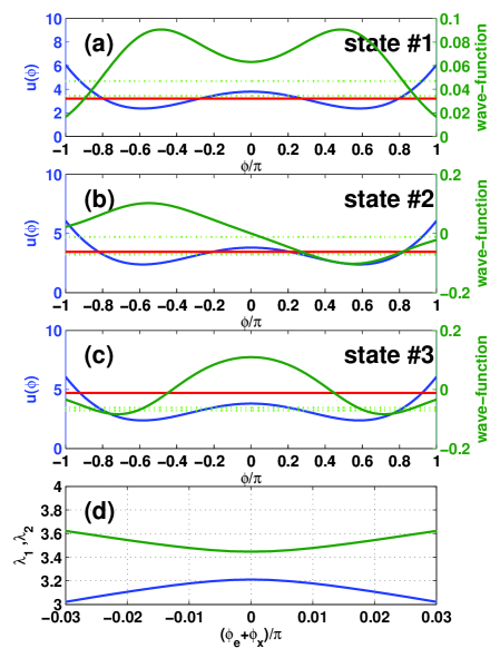
Figure 2: (Color online) Eigenstates of $\mathcal{H}_{1}$. (a)-(c) The first 3 lowest energy states for the case $\phi_{e}+\phi_{x}=0$. (d) The energy of the two lowest states vs. $\phi_{e}+\phi_{x}$.

From these results one finds for the values of the $\eta$ and $\Delta$ parameters in the two-level approximation to Hamiltonian $\mathcal{H}_{1}$ [Eq. (22)],

$$\eta =2.5U_{0}\ ,$$ (76a)

$$\Delta =0.12U_{0}\ .$$ (76b)

Using these values yields

$$x_{0} =4.1\times 10^{-6}\operatorname{nm}\ ,$$ (77a)

$$\zeta =2.5\times 10^{-4}\ ,$$ (77b)

$$\frac{x_{0}}{x_{\phi}} =2.0\times 10^{-6}\ ,$$ (77c)

$$\alpha_{0} =0.18\ ,$$ (77d)

$$\left\langle n\right\rangle =1.2\ ,$$ (77e)

$$\left(\zeta\alpha_{0}\omega_{0}\right)^{-1} =5.6\operatorname{\mu s}\ ,$$ (77f)

$$\frac{4\pi}{\zeta Q}\left(\frac{x_{0}}{\lambda_{T}}\right)^{2} =1.0\ ,$$ (77g)

$$\frac{2\pi}{\zeta\omega_{0}} =6.3\operatorname{\mu s}\ ,$$ (77h)

$$\frac{x_{\phi}}{2x_{0}\beta_{h}}\frac{\Delta^{2}}{\eta U_{0}} =3.0\times 10^{6}\ .$$ (77i)

Eqs. (77f) and (77g) indicate that observation of both decoherence and recoherence, for the case of the present example, is feasible, provided that the decoherence time of the RF SQUID due to other mechanisms is sufficiently long, i.e., on the order of microseconds Yoshihara et al. (2006). Moreover, Eq. (77i) ensures the validity of the adiabatic approximation.

X Discussion and Conclusions

A possible, alternative protocol to the presently considered one for observing decoherence/recoherence phenomena is the so-called Ramsey interference experiment that proceeds as follows Armour et al. (2002) : (i) At time $t<0$, the state is prepared in the ground state $\left|\curvearrowright\right\rangle$, identically to the above considered protocol by applying an external bias flux $\phi_{e}$ such that $\phi_{e}\gg\Delta/\eta$ ; (ii) At time $t=0$, the external flux $\phi_{e}$ is suddenly switched to the new value $\phi_{e}=0$, again just as in the above protocol, but then after one-quarter of a Rabi oscillation period, $\phi_{e}$ is suddenly switched back up to the same non-zero value as was applied during first, preparation stage; (iii) The flux qubit and mechanical oscillator are then left to interact for a certain duration with $\phi_{e}$ kept constant; (iv) Stage (ii) is repeated again; (v) The state of the qubit is read out.

The effect of stage (ii) is to prepare the flux qubit in a state which is an equal magnitude superposition of the circulating current states $\left|\curvearrowright\right\rangle$ and $\left|\curvearrowleft\right\rangle$. Each of these states is associated with the different spatially-shifted potentials $V_{\pm}(x)$ [Eq. (28)], so that during the interaction stage (iii) an entangled state develops between the oscillator and flux qubit, giving rise to decoherence of the reduced qubit state. After one full mechanical period, the entanglement is undone, resulting in recoherence. The second, quarter Rabi period pulse enables one to probe the decoherence/recoherence, simply by measuring the probability to be in one of the measurement basis states, e.g., the ground state $\left|\curvearrowright\right\rangle$. By repeating the Ramsey protocol many times, allowing the interaction duration to range over several mechanical periods, oscillations in the visibility are observed providing a signature of decoherence/recoherence.

The Ramsey protocol has the obvious advantage over the above considered protocol (where one always remains at the $\phi_{e}=0$ degeneracy point during $t>0$) that the decoherence/recoherence times are shorter by the factor of $1/\zeta$. However, the disadvantage with the Ramsey protocol is that qubit decoherence times are considerably reduced away from the degeneracy point. The origin of the reduction in these two competing timescales is of course the same: the mechanical oscillator and flux noise couple more strongly (i.e., linear coupling) to the circulating current basis states $\left|\curvearrowright\right\rangle$ and $\left|\curvearrowleft\right\rangle$ than to the eigenstate basis states at the degeneracy point (i.e., quadratic coupling). Depending on how the qubit decoherence rate varies with the externally applied flux, it may be that operating a small distance from the degeneracy point is more favorable for observing recoherence effects Yoshihara et al. (2006). However, the resulting coupled quantum dynamics is not as simple to describe as at the special limiting bias points where the Hamiltonian $\mathcal{H}_{1}$ [Eq. (22)] is either (approximately) purely diagonal or off-diagonal.

In the present paper we have considered a flux qubit in the form of an RF SQUID, a system that is relatively simple to analyze. However, a double well potential can be formed only when the inductance $L$ is sufficiently large and the condition $\beta_{L}>1$ is satisfied. In this limit, the loop is relatively large and consequently large pickup of external flux noise results in a relatively short flux qubit decoherence time Friedman et al. (2000). On the other hand, this problem can be partly solved by employing the configuration of a loop having three JJs Mooij et al. (1999), where a portion of the necessary total SQUID inductance is provided by the effective inductance of the additional JJs; the three JJ superconducting loop would likely be the preferred choice for experimental implementation.

XI Acknowledgements

This work is partly supported by the US - Israel Binational Science Foundation (BSF) and by the Israeli ministry of science. M. P. B. thanks the Aspen Center for Physics for their hospitality and support.

References

• Leggett (2002) A. J. Leggett, J. Phys. Condens. Matter 14, R415 (2002).
• Leggett and Garg (1985) A. J. Leggett and A. Garg, Phys. Rev. Lett. 54, 857 (1985).
• Armour and Blencowe (2001) A. D. Armour and M. P. Blencowe, Phys. Rev. B 64, 035311 (2001).
• Bose et al. (1997) S. Bose, K. Jacobs, and P. L. Knight, Phys. Rev. A 56, 4175 (1997).
• Mancini et al. (1997) S. Mancini, V. I. Man’ko, and P. Tombesi, Phys. Rev. A 55, 3042 (1997).
• Marshall et al. (2003) W. Marshall, C. Simon, R. Penrose, and D. Bouwmeester, Phys. Rev. Lett. 91, 130401 (2003).
• Bernad et al. (2006) J. Z. Bernad, L. Diosi, and T. Geszti, arXiv: quant-ph/0604157 (2006).
• Armour et al. (2002) A. D. Armour, M. P. Blencowe, and K. C. Schwab, Phys. Rev. Lett. 88, 148301 (2002).
• Cleland and Geller (2004) A. N. Cleland and M. R. Geller, Phys. Rev. Lett. 93, 070501 (2004).
• Zhou and Mizel (2006) X. Zhou and A. Mizel, quant-ph/0605017 (2006).
• Xue et al. (2006) F. Xue, Y. Wang, C.P.Sun, H. Okamoto, H. Yamaguchi, and K. Semba, arXiv: cond-mat/0607180 (2006).
• Moody et al. (1989) J. Moody, A. Shapere, and F. Wilczek, in Geometric Phases in Physics, edited by A. Shapere and F. Wilczek (World Scientific Publishing Co., Singapore, 1989), p. 160.
• Glauber (1969) R. J. Glauber, Quantum Optics (Academic Press, 1969).
• Caldeira and Leggett (1983) A. O. Caldeira and A. J. Leggett, Physica A 121, 587 (1983).
• Joos and Zeh (1985) E. Joos and H. D. Zeh, Physik B 59, 223 (1985).
• Unruh and Zurek (1989) W. G. Unruh and W. H. Zurek, Phys. Rev. D 40, 1071 (1989).
• Zurek (1991) W. H. Zurek, Physics Today 44, 36 (1991).
• Buks (2006) E. Buks, J. Opt. Soc. Am. B 23, 628 (2006).
• Friedman et al. (2000) J. R. Friedman, V. Patel, W. Chen, S. K. Tolpygo, and J. E. Lukens, Nature 406, 43 (2000).
• Roukes (2000) M. L. Roukes, arXiv: cond-mat/0008187 (2000).
• Yoshihara et al. (2006) F. Yoshihara, K. Harrabi, A. O. Niskanen, Y. Nakamura, and J. S. Tsai, arXiv: cond-mat/0606481 (2006).
• Mooij et al. (1999) J. E. Mooij, T. P. Orlando, L. Levitov, L. Tian, C. H. V. der Wal, and S. Lloyd, Science 285, 1036 (1999).