Quantum walks with random phase shifts

Abstract

We investigate quantum walks in multiple dimensions with different quantum coins. We augment the model by assuming that at each step the amplitudes of the coin state are multiplied by random phases. This model enables us to study in detail the role of decoherence in quantum walks and to investigate the quantum-to-classical transition. We also provide classical analogues of the quantum random walks studied. Interestingly enough, it turns out that the classical counterparts of some quantum random walks are classical random walks with a memory and biased coin. In addition random phase shifts “simplify” the dynamics (the cross interference terms of different paths vanish on average) and enable us to give a compact formula for the dispersion of such walks.

I Introduction

The concept of quantum walks (QW) has been introduced (see Ref. ADZ93a ) in order to explore how the intrinsically statistical character of quantum mechanics affects statistical properties of quantum analogues of classical random walks. In particular, an example of a random process is a Markov chain such that the position value $x\in X$ is iteratively updated, given by the transition probability $P(x|y)$.

Quantum walks have been studied in connection with novel quantum algorithms: The instances thereof were provided in Ref. shenvi:052307 (the quantum walk algorithm on the hypercube with complexity $O(\sqrt{n})$) and in Ref. CE03a (the quantum walk algorithm for subset finding). The former uses the quantum walk on the hypercube, while the latter uses the quantum walk on bipartite graphs. Quantum walks on bipartite graphs were analyzed in Ref. szeg:0401053 .

Various aspects of QWs have been studied in detail recently (for a review on QWs see Ref. Kempe2003 ). In particular, Aharonov et al. have presented an analytic description of discrete quantum walks on Cayley graphs AAKV01a . A special case of a Cayley graph, the line, was asymptotically analyzed in Ref. ABN+01a . It has been shown that, unlike classical random walks, the probability distribution induced by quantum walks is not Gaussian (with a peak around the origin of the walk), but has two peaks at positions $\pm\frac{n}{\sqrt{2}}$, where $n$ is the number of steps. As a result the dispersion of probability distribution for quantum walks grows quadratically, compared to linear growth for classical random walks. The role of decoherence in quantum walks has been analyzed by Kendon et al. Ref. Kendon2002 ; Kendon2003

Quantum walks are intrinsically deterministic processes (in the same sense as the Schrödinger equation is a deterministic equation). Their “classical randomness” only emerges when the process in monitored (measured) in one way or another. Via the measurement, one can regain a classical behavior for the process. For instance, by measuring the quantum coin, the quadratic dispersion of the probability distribution reverts to a classical, linear dispersion. If the quantum coin is measured at every step, then the record of the measurement outcomes singles out a particular classical path. By averaging over all possible measurement records, one recovers the usual classical behavior brun:052317 ; BCA02b . Instead of measuring the quantum coin after each step, an alternative way to regain classical randomness from a quantum walk is to replace this coin with a new quantum coin for each flip.

After $n$ steps of the walk one accumulates $n$ coins that are entangled with the position of the walking particle. By measuring a set of $n$ quantum coins, one could reconstruct a unique classical trajectory and by averaging over all possible measurement outcomes, one once again recovers the classical result.

These two approaches to regaining classical behavior from the quantum walk have been contrasted in a recent work by Brun et al. BCA02b . This comparison has been studied for the particular example of a discrete walk on the line.

In the present paper we analyze the quantum-to-classical transition using random phase shifts on the coin register. In Sec. II we give an introduction to the quantum walk model. In Sec. III (part A) we augment the model by random phase shift dynamics and present the solution in terms of path integrals. It turns out that on average the interference of amplitudes of different paths is zero and we derive the formula for the dispersion of the mean probability distribution in compact form. We contrast the dynamics of quantum walks with two coins (permutation symmetric and Fourier transform) with the dynamics of classical random walks and find an equivalence between the two (considering the possibility that the CRW has memory and a biased coin). In part B of Sec. III we provide the numerical results of the problem. In particular, we briefly analyze a situation in which phases of random shifts are distributed according to a normal distribution that is peaked around the phase zero and with the dispersion $\sigma$. When the dispersion is zero, (i.e. $\sigma=0$) we recover the QW, while for large $\sigma$, we obtain a uniform distribution on the interval $[-\pi,\pi]$ and the CRW is recovered. In between we can observe a continuous quantum-to-classical transition of quantum walks. In Sec. IV we present our conclusions. Some technical details of the calculations can be found in Appendix A.

II QW in multiple dimensions

Let us first define a quantum walk in $d$ dimensions – i.e. on the lattice $\mathbb{Z}^{d}$. The quantum walk is generated by a unitary operator repeatedly applied on a vector from a Hilbert space $\mathcal{H}\equiv\mathcal{H}_{X}\otimes\mathcal{H}_{D}$. The Hilbert space $\mathcal{H}_{X}\equiv\text{span}\{|\mathbf{x}\rangle:\mathbf{x}\in\mathbb{Z}^{d}\}$ is called the position Hilbert space. For $\forall\mathbf{x},\mathbf{y}\in\mathbb{Z}^{d}$ we define the usual scalar product $\mathbf{x}\cdot\mathbf{y}\equiv\sum_{j=1}^{d}\mathbf{x}_{j}\mathbf{y}_{j}$ and the norm $|\mathbf{x}|=\sqrt{\mathbf{x}\cdot\mathbf{x}}$. In the following, the distance between the vertices is a dimensionless quantity, with the distance between adjacent vertices equal to 1.

There are $2d$ vectors $\mathbf{e}_{a}\in\mathbb{Z}^{d}$ such that $|\mathbf{e}_{a}|=1$. The space $\mathcal{H}_{D}\equiv\text{span}\{|a\rangle:a=1,\dots,2d\}$ is spanned by states isomorphic to $\mathbf{e}_{a}$. $\mathcal{H}_{D}$ is called the direction Hilbert space. In the following we set $D=\{1,\dots,2d\}$.

A single step of quantum walk is generated by the unitary operator $U$ such that $U=S(1\otimes C)$, where

$$S=\sum_{\mathbf{x}\in\mathbb{Z}^{d}}\sum_{a\in D}|\mathbf{x}+\mathbf{e}_{a}\rangle\langle\mathbf{x}|\otimes|a\rangle\langle a|\equiv\sum_{a\in D}T_{a}\otimes P_{a}\;;$$ (1)

$P_{a}\equiv|a\rangle\langle a|$ and $C$ is any unitary operator. The operator $S$ changes the state of the position register in the direction $a$, while the coin operator $C$ operates on the direction register. For simplicity we consider the permutation symmetric coin

$$C=\left[\begin{matrix}r&t&t&\dots\\ t&r&t&\dots\\ \vdots&\vdots&\ddots&\dots&\\ t&\dots&t&r\end{matrix}\right]\;.$$ (2)

The quantum walk is generated by a sequence $U^{n}|\psi_{0}\rangle$, where $|\psi_{0}\rangle$ is some initial state. For simplicity, we assume

$$|\psi_{0}\rangle=|\mathbf{0}\rangle\otimes|s\rangle\;,$$ (3)

where $|s\rangle\equiv\frac{1}{\sqrt{|D|}}\sum_{a\in D}|a\rangle$. We also assume the so-called Grover coin MR02a , which is a specific instance of the permutation symmetric coin in Eq. (2), described by the operator

$$C_{G}=2|s\rangle\langle s|-1\;.$$ (4)

In order to find the eigensystem of $U$, we switch to the translationally symmetric basis AAKV01a . We set

$$|\tilde{\phi}_{\mathbf{k}}\rangle=\sum_{\mathbf{x}\in\mathbb{Z}^{d}}e^{i\mathbf{k}\cdot\mathbf{x}}|\mathbf{x}\rangle\;,$$ (5)

where $\mathbf{k}\in\mathbb{R}^{d}$. By virtue of the inverse Fourier transform we obtain

$$|\mathbf{x}\rangle=\frac{1}{(2\pi)^{d}}\int_{-\pi}^{\pi}e^{-i\mathbf{k}\cdot\mathbf{x}}|\tilde{\phi}_{\mathbf{k}}\rangle d^{d}\mathbf{k}\;,$$ (6)

with $|\tilde{\phi}_{\mathbf{k}}\rangle$ are eigenvectors of the translation operator in the $a$-th direction, i.e.

$$T_{a}|\tilde{\phi}_{\mathbf{k}}\rangle=e^{-i\mathbf{k}\cdot\mathbf{e}_{a}}|\tilde{\phi}_{\mathbf{k}}\rangle\;,$$ (7)

where $T_{a}=\sum_{\mathbf{x}\in\mathbb{Z}^{d}}|\mathbf{x}+\mathbf{e}_{a}\rangle\langle\mathbf{x}|$. By applying the evolution operator, we obtain

$$\begin{split}U|\tilde{\phi}_{\mathbf{k}}\rangle\otimes|\chi\rangle&=S|\tilde{\phi}_{\mathbf{k}}\rangle\otimes C|\chi\rangle\\ &=\sum_{a\in D}e^{-i\mathbf{k}\cdot\mathbf{e}_{a}}|\tilde{\phi}_{\mathbf{k}}\rangle\otimes|a\rangle\langle a|C|\chi\rangle\\ &=|\tilde{\phi}_{\mathbf{k}}\rangle\otimes\Lambda_{k}C|\chi\rangle\;,\end{split}$$ (8)

where

$$\Lambda_{k}=\sum_{a\in D}e^{-i\mathbf{k}\cdot\mathbf{e}_{a}}|a\rangle\langle a|\;.$$ (9)

In order to simplify the notation in what follows we will denote projectors $|a\rangle\langle a|$ as $P_{a}$. To find the eigensystem of $U$, we need to find the eigensystem of $\Lambda_{k}C$. Equivalently, we need to evaluate $(\Lambda_{k}C)^{n}|\chi\rangle$.

We first use the Grover matrix $C_{G}$ in Eq. (4). In order to find the power of the matrix $(\Lambda_{\mathbf{k}}C_{G})^{n}$ we prove the following lemma:

Lemma 1.

Let ${\cal D}=\{|a\rangle\}$ be the orthonormal basis of a Hilbert space and $C_{G}=2P_{s}-1$, where $|s\rangle=\frac{1}{\sqrt{|D|}}\sum_{a\in D}|a\rangle$. Then

$$\left(P_{a}C_{G}\right)^{n}=p_{n}|a\rangle\langle s|+q_{n}P_{a}\;,$$

with $p_{n}=\frac{2}{\sqrt{|D|}}\left(\frac{2}{|D|}-1\right)^{n-1}$ and $q_{n}=-\left(\frac{2}{|D|}-1\right)^{n-1}$.

Proof.

We denote $P_{a}C_{G}=\frac{2}{\sqrt{|D|}}|a\rangle\langle s|-P_{a}=p_{0}|a\rangle\langle s|+q_{0}P_{a}$. Setting $(P_{a}C_{G})^{k}=p_{k}|a\rangle\langle s|+q_{k}P_{a}$ we get that $p_{k+1}=p_{k}\big{(}\frac{2}{|D|}-1\big{)}$ and $q_{k+1}=q_{k}\big{(}\frac{2}{|D|}-1\big{)}$. By induction we immediately obtain the result. ∎

From Eq. (9) we see that with the Grover coin

$$\begin{split}&(\Lambda_{\mathbf{k}}C_{G})^{n}=\bigg{(}\sum_{a\in D}e^{-i\mathbf{k}\cdot\mathbf{e}_{a}}P_{a}C_{G}\bigg{)}^{n}=\\ &=\sum_{(a_{1},\dots,a_{n})\in D^{n}}e^{-i\mathbf{k}\cdot(\mathbf{e}_{a_{1}}+\dots+\mathbf{e}_{a_{n}})}P_{a_{1}}C_{G}\dots P_{a_{n}}C_{G}\;.\end{split}$$ (10)

By induction, the expression $P_{a_{1}}C_{G}\dots P_{a_{n}}C_{G}$ from Eq. (10) can be rewritten as

Lemma 2.

$$\begin{split}&P_{a_{1}}C_{G}\dots P_{a_{n}}C_{G}=\frac{(-1)^{n}}{|D|^{(2n-1)/2}}\\ &\times\prod_{j=1}^{n-1}(|D|\delta_{a_{j},a_{j+1}}-2)(\sqrt{|D|}|a_{1}\rangle\langle a_{n}|-2|a_{1}\rangle\langle s|)\;.\end{split}$$ (11)

The product in Eq. (11) is taken to be 1 for $n=1$.

Alternatively, in Eq. (10), the last line can be rewritten as

$$\begin{split}&P_{a_{1}}C_{G}\dots P_{a_{n}}C_{G}\\ &=\prod_{\begin{subarray}{c}m_{1}+\dots+m_{k}=n\\ (a^{(1)},\dots,a^{(k)})\in D^{k}\end{subarray}}(P_{a^{(1)}}C_{G})^{m_{1}}\dots(P_{a^{(k)}}C_{G})^{m_{k}}\;,\end{split}$$ (12)

where $a^{(j)}\in D$. According to Lemma 1 all the terms in the product in Eq. (12) can be expressed as the linear combination of $|a^{(j)}\rangle\langle s|,P_{a^{(j)}}$. Since for $j\neq j^{\prime}\Rightarrow\langle a^{(j)}|a^{(j^{\prime})}\rangle=0$, we get the result

$$\begin{split}&(\Lambda_{\mathbf{k}}C_{G})^{n}=\sum_{\text{partition}}e^{-i\mathbf{k}\cdot(\mathbf{e}_{a^{(1)}}+\dots+\mathbf{e}_{a^{(k)}})}\\ &\times\bigg{(}S(m_{1},\dots,m_{k})|a_{1}\rangle\langle s|+T(m_{1},\dots,m_{k})P_{a_{n}}\bigg{)}\;.\end{split}$$ (13)

The expressions for $S$ and $T$ are given by relations

$$S(m_{1},\dots,m_{k}) = p_{m_{1}}\dots p_{m_{k}}\;;$$ (14)

$$T(m_{1},\dots,m_{k}) = p_{m_{1}}\dots p_{m_{k-1}}q_{m_{k}}\;,$$ (15)

where we use the notation of Lemma 1. The coefficients $m_{1},\dots,m_{k}$ give the partitioning of the integer $n$ such that $m_{1}+\dots+m_{k}=n$. The “partition” in Eq. (13) means the summation over all such partitions.

Starting with the initial state $|\psi_{0}\rangle=|\mathbf{0}\rangle\otimes|s\rangle$ and using the expression (11), we obtain

$$\begin{split}&(\Lambda_{\mathbf{k}}C_{G})^{n}|s\rangle=\\ &=\sum_{(a_{1},\dots,a_{n})\in D^{n}}e^{-i\mathbf{k}\cdot(\mathbf{e}_{a_{1}}+\dots+\mathbf{e}_{a_{n}})}\frac{(-1)^{n+1}}{|D|^{(2n-1)/2}}\\ &\times\Big{[}\prod_{j=1}^{n-1}(|D|\delta_{a_{j},a_{j+1}}-2)\Big{]}|a_{1}\rangle\;.\end{split}$$ (16)

This equation takes the singular form for $|D|=2$ (i.e. , for one-dimensional quantum walk on line) such that only the summands for which all elements $\{a_{1},\dots,a_{n}\}$ are distinct, contribute to the total sum. As a consequence, the sum in Eq. (16) when $|D|=2$ is zero for $n>2$. But this case is special in that the coefficient $r$ of the Grover matrix is zero. From now on we will consider the dimension of the lattice to be equal or larger than $2$, so that, $|D|\geq 4$.

The expression (16) is symmetric with respect to the permutation of elements, i.e. , $\langle a_{j}|(\Lambda_{\mathbf{k}}C_{G})^{n}|s\rangle$ has the same value for any $a_{j}\in D,n\in\mathbb{Z}$. A value of the right-hand side of Eq. (16) depends on the term

$$\Xi_{0}(a_{1},\dots,a_{n})=\prod_{j=1}^{n-1}(|D|\delta_{a_{j},a_{j+1}}-2)\;.$$ (17)

Obviously, $\left|\Xi_{0}(a_{1},\dots,a_{n})\right|$ is maximal for $a_{1}=\dots=a_{n}$. More precisely, if $a_{j}=a_{j+1}$ for $j=0,\dots,n-1$ in Eq. (17), then

$$\left|\Xi_{0}(a_{1},\dots,a_{n})\right|=O\left((|D|-2)^{k}\;2^{n-k}\right)\;,$$ (18)

and there are $O\left(|D|^{n}\right)$ such terms in the sum of Eq.  (16). Now Eq. (16) takes the form

$$\begin{split}&(\Lambda_{\mathbf{k}}C_{G})^{n}|s\rangle=\\ &=\frac{(-1)^{n+1}}{|D|^{(2n-1)/2}}\sum_{(a_{1},\dots,a_{n})\in D^{n}}e^{-i\mathbf{k}\cdot(\mathbf{e}_{a_{1}}+\dots+\mathbf{e}_{a_{n}})}\Xi_{0}(a_{1},\dots,a_{n})|a_{1}\rangle\;.\end{split}$$ (19)

In what follows we will compare the quantum walk described by Eq. (8) with the quantum walk with random phase shifts.

III QW with random phase shifts

III.1 Analytic Results

Quantum walks differ from classical random walks (CRW) in many respects. One of the main differences is that dispersions of probability distributions of CRW grow linearly with the number of steps while for QW the dispersions grow quadratically ABN+01a . In what follows we will show that introducing random phase shifts (RPS) at each step of the evolution causes the QW to behave more like a classical random walk. The reduction of the QW to the CRW has been discussed in Refs. brun:052317 ; BCA02b . The authors of these papers have discussed two possible routes to classical behavior for the discrete QW on a line. First, the QW-to-CRW transition has been considered as a result of decoherence in the quantum “coin” which drives the walk. Second, higher-dimensional coins have been used to “dilute” the effects of quantum interference. The position variance has been used as an indicator of classical behavior. It has been shown that the multi-coin walk retains the “quantum” quadratic growth of the variance except in the limit of a new coin for every step, while the walk with decoherence exhibits “classical” linear growth of the variance even for weak decoherence.

In what follows we will utilize a different approach to analyze the QW-to-CRW transition. In Ref. BCA02b the authors used a CP-map on the coin degree of freedom to simulate the effects of decoherence on the quantum walks in 1 dimension. If the CP map is pure dephasing, then the dispersion of the probability distribution is asymptotically linear. Our approach is new in two respects: Firstly, we generalize the problem to an arbitrary number of dimensions; secondly we apply a different map, a sequence of random phase shifts on the coin. We assume that at each step a random phase shift ($\theta_{a}^{(n)}$) described by a unitary operator

$$R(\theta^{(n)})=\sum_{a\in D}e^{i\theta_{a}^{(n)}}P_{a}$$ (20)

on the direction register is applied to a particle. This procedure, in effect, is equivalent to an application of another (random) coin on the whole direction register. Each random sequence $\Sigma\equiv\{R(\theta^{(n)})\}_{n=1}^{\infty}$ generates a different quantum walk

$$U(\theta^{(1)})\cdots U(\theta^{(n)})=\prod_{m=1}^{n}S\cdot\left(1\otimes R(\theta^{(j)})C\right)\;.$$ (21)

As we shall see later on, particular random walk probability distributions associated with different sequences of random phase shifts do not differ significantly.

What is significant on the QW-RPS is that it has mixing properties similar to the classical random walk (the linear growth of variance) and in particular for dimension = 2, the mean probability distribution is exactly the same as for the classical random walk. Before we prove both statements, we derive the formula for the dispersion of the probability distribution for QW-RPS, using a generalized Grover (i.e. permutation symmetric) coin.

The generalized Grover coin is (cf. Eq. (2))

$$G_{r,t}=r\sum_{a\in D}P_{a}+t\sum_{\begin{subarray}{c}a,b\in D\\ a\neq b\end{subarray}}|a\rangle\langle b|=(r-t)\mathbb{I}+t|D|P_{s}\;.$$ (22)

where $P_{a}=|a\rangle\langle a|$. This operator is unitary iff the following relations hold:

$$|r|^{2}+(|D|-1)|t|^{2} = 1\;;$$ (23)

$$(|D|-2)|t|^{2}+r^{*}t+rt^{*} = 0\;.$$ (24)

The QW-RPS may be thought of as a sequence of random operators $U(\theta)$ such that

$$U_{r,t}(\theta)=\left[\sum_{a\in D}T_{a}\otimes P_{a}\right]\;\cdot\;(1\otimes\widehat{C}(\theta))\;,$$ (25)

and

$$\widehat{C}(\theta)=1\otimes\sum_{a\in D}e^{i\theta_{a}}P_{a}G_{r,t}\;.$$ (26)

Here $\theta=(\theta_{1},\dots,\theta_{|D|})$ is a sequence of independent random real variables. Hence we actually get a sequence of random operators $\{U(\theta^{(j)})\}_{j}$ which creates the QW-RPS.

One step of a QW-RPS is given by:

$$\begin{split}U_{r,t}(\theta^{(1)})&=S\cdot\widehat{C}(\theta^{(1)})=\Big{(}\sum_{a_{1}\in D}T_{a_{1}}\otimes|a_{1}\rangle\langle a_{1}|\Big{)}\\ &\times\Big{[}1\otimes\sum_{a\in D}e^{i\theta^{(1)}_{a}}({t}{\sqrt{|D|}}|a\rangle\langle s|+(r-t)P_{a})\Big{]}\\ &=\sum_{a_{1}\in D}T_{a_{1}}\otimes e^{i\theta^{(1)}_{a_{1}}}\Big{(}{t}{\sqrt{|D|}}|a_{1}\rangle\langle s|+(r-t)P_{a_{1}}\Big{)}\;.\end{split}$$ (27)

For the chain of $n$ evolution operators of QW-RPS we obtain

Lemma 3.

Let $\{U_{r,t}(\theta^{(j)})\}_{j=1}^{\infty}$ be a sequence of random operators according to Eq. (25). Then

$$\begin{split}&U_{r,t}(\theta^{(1)})\cdots U_{r,t}(\theta^{(n)})=\sum_{a_{1},\dots,a_{n}\in D}T_{a_{1}+\dots+a_{n}}\\ &\otimes e^{i(\theta^{(1)}_{a_{1}}+\dots+\theta^{(n)}_{a_{n}})}\Big{[}(r-t)|a_{1}\rangle\langle a_{n}|+{t}{\sqrt{|D|}}|a_{1}\rangle\langle s|\Big{]}\\ &\times\Xi(a_{1},\dots,a_{n})|a_{1}\rangle\;,\end{split}$$ (28)

where

$$\Xi(a_{1},\dots,a_{n})\equiv\prod_{j=1}^{n-1}\Big{[}{t}+(r-t)\delta_{a_{j},a_{j+1}}\Big{]}\;.$$ (29)

Proof.

By induction. ∎

It can be analyzed how a specific QW-RPS evolves given a specific initial state $|\psi_{0}\rangle=|\mathbf{0}\rangle\otimes|s\rangle$.

Lemma 4.

Let $\{U(\theta^{(j)})\}_{j=1}^{\infty}$ be a sequence of random operators according to Eq. (25). Then

$$\begin{split}&|\psi(\Theta,n)\rangle\equiv U(\theta^{(1)})\cdots U(\theta^{(n)})|\mathbf{0}\rangle\otimes|s\rangle=\\ &=\sum_{a_{1},\dots,a_{n}\in D}|\mathbf{0}+\mathbf{e}_{a_{1}}+\dots+\mathbf{e}_{a_{n}}\rangle\otimes\\ &\otimes e^{i(\theta^{(1)}_{a_{1}}+\dots+\theta^{(n)}_{a_{n}})}\Xi(a_{1},\dots,a_{n})\Big{[}\frac{r-t}{\sqrt{|D|}}+\sqrt{|D|}t\Big{]}|a_{1}\rangle\;.\end{split}$$ (30)

Proof.

From Lemma 3.

∎

The probability distribution of $|\psi(\Theta,\mathbf{x},n)\rangle$ shall be derived by projecting it onto $P_{\mathbf{x}}\otimes 1$ and tracing over the coin Hilbert space. Hence by setting

$$\mathbf{a} \equiv (a_{1},\dots,a_{n})$$ (31)

$$\mathbf{a}^{\prime} \equiv (a_{1}^{\prime},\dots,a_{n}^{\prime})$$ (32)

$$\theta(\mathbf{a}) \equiv (\theta_{a_{1}}+\dots+\theta_{a_{n}})$$ (33)

we get

$$\begin{split}P(\Theta,&\mathbf{x},n)=\|(P_{\mathbf{x}}\otimes 1)\psi(\Theta,n)\|^{2}=\Big{|}\frac{r-t}{\sqrt{|D|}}+\sqrt{|D|}t\Big{|}^{2}\times\\ &\times\sum_{\begin{subarray}{c}\mathbf{a},\mathbf{a}^{\prime}\in D^{n}\\ \mathbf{a}\equiv\mathbf{x}\equiv\mathbf{a}^{\prime}\end{subarray}}e^{i(\theta(\mathbf{a})-\theta(\mathbf{a}^{\prime}))}\Xi(\mathbf{a})\Xi(\mathbf{a}^{\prime})^{*}\langle a_{1}|a_{1}^{\prime}\rangle\;,\end{split}$$ (34)

where $\theta(\mathbf{a})$ is the sum of the sequence of independent random variables for each $\mathbf{a}$ and $\Xi$ is the same as in Eq. (17). The symbol $\mathbf{a}\equiv\mathbf{x}$ means that $\mathbf{0}+\sum_{j=1}^{n}\mathbf{e}_{a_{j}}=\mathbf{x}$. It is clear that $P(\Theta,\mathbf{x},n)=P(\Theta,\mathbf{x},n)^{*}$ since we are summing over all tuples $\mathbf{a},\mathbf{a}^{\prime}$.

Eq. (34) depends on $\Theta$, which is an event generating $n|D|$ random variables $\{\theta_{a_{j}}:j=1,\dots,n,\;a\in\mathbf{a}\}$. We can split Eq. (34) into two parts:

$$\begin{split}P(&\Theta,\mathbf{x},n)=\Big{|}\frac{r-t}{\sqrt{|D|}}+\sqrt{|D|}t\Big{|}^{2}\Big{\{}\sum_{\begin{subarray}{c}\mathbf{a}\in D^{n}\\ \mathbf{a}\equiv\mathbf{x}\equiv\mathbf{a}^{\prime}\end{subarray}}|\Xi(\mathbf{a})|^{2}+\\ &+\sum_{\begin{subarray}{c}\mathbf{a}\neq\mathbf{a}^{\prime}\\ \mathbf{a}\equiv\mathbf{x}\equiv\mathbf{a}^{\prime}\end{subarray}}e^{i(\theta(\mathbf{a})-\theta(\mathbf{a}^{\prime}))}\Xi(\mathbf{a})\Xi(\mathbf{a}^{\prime})^{*}\langle a_{1}|a_{1}^{\prime}\rangle\Big{\}}\end{split}$$ (35)

To obtain the mean probability distribution, we integrate over the random variable $\theta$,assuming uniform distribution for all phases of $\theta$:

$$\begin{split}\langle P(\Theta,\mathbf{x},n)\rangle_{\Theta}&=\int_{0}^{2\pi}\frac{d^{|D|n}\theta}{(2\pi)^{|D|n}}P(\Theta,\mathbf{x},n)\\ &=\Big{|}\frac{r-t}{\sqrt{|D|}}+\sqrt{|D|}t\Big{|}^{2}\sum_{\begin{subarray}{c}\mathbf{a}\in D^{n}\\ \mathbf{a}\equiv\mathbf{x}\equiv\mathbf{a}^{\prime}\end{subarray}}|\Xi(\mathbf{a})|^{2}\;.\end{split}$$ (36)

The terms coming from $\sum_{\begin{subarray}{c}\mathbf{a}\neq\mathbf{a}^{\prime}\\ \mathbf{a}\equiv\mathbf{x}\equiv\mathbf{a}^{\prime}\end{subarray}}$ cancel out. Now the mean probability distribution depends only on the term $\Xi(\mathbf{a})$. For $d=2$ and Grover coin (i.e. $r=\frac{2}{|D|}-1,\;t=\frac{2}{|D|}$), this term is the product of $\pm 2$, and $|\Xi(\mathbf{a})|^{2}=2^{-2(n-1)}$. Then

$$\langle P(\Theta,\mathbf{x},n)\rangle_{\Theta}=\frac{1}{4^{n}}\sum_{\begin{subarray}{c}\mathbf{a}\in D^{n}\\ \mathbf{a}\equiv\mathbf{x}\end{subarray}}1\;.$$ (37)

The sum over all paths in Eq. (37) is the same as the sum of all classical paths. The constant is the product of the probability to take any individual direction at each step. Hence the mean probability distribution of QW-RPS for dimension 2 is the same as the CRW in 2 dmensions. We easily show that the probability distribution resulting from Eq. (37) is normalized:

$$\sum_{\mathbf{x}\in\mathbb{Z}^{d}}\langle P(\Theta,\mathbf{x},n)\rangle_{\Theta}=\frac{1}{4^{n}}\sum_{\mathbf{a}\in D^{n}}1=1\;.$$ (38)

It is an interesting question whether the equivalence of QW-RPS with CRW in two dimensions is merely a coincidence, or whether the same result applies for higher dimensions with a modified Grover coin.

Now we arrive at the conclusion that the averaged probability distribution of QW-RPS with the generalized Grover coin $G_{r,t}$, is

$$\langle P(\Theta,\mathbf{x},n)\rangle_{\Theta}=\Big{|}\frac{r-t}{\sqrt{|D|}}+\sqrt{|D|}t\Big{|}^{2}\,\sum_{\begin{subarray}{c}\mathbf{a}\in D^{n}\\ \mathbf{a}\equiv\mathbf{x}\end{subarray}}|\Xi(\mathbf{a})|^{2}\;.$$ (39)

This equation is one of the main results of our paper, as it shows that the probability distribution of a QW-RPS corresponds to a classical sum over paths.

In order to study specific properties of the mean probability distribution let us consider its dispersion that is defined as

$$\mathcal{D}(D,n)=\sum_{\mathbf{x}\in\mathbb{Z}^{d}}\langle P(\Theta,\mathbf{x},n)\rangle_{\Theta}|\mathbf{x}|^{2}.$$ (40)

The dispersion corresponding to the mean probability distribution is evaluated in Appendix A [see Eq. (68)] from which we can derive the following theorem:

Theorem 5.

The dispersion of QW-RPS with a generalized Grover coin with coefficients $r$,$t$ for $n>2$ is

$$\mathcal{D}(D,n)=\frac{1+|r|^{2}-|t|^{2}}{1-|r|^{2}+|t|^{2}}(n-2)+O\Big{(}(|r|^{2}-|t|^{2})^{n}\Big{)}$$ (41)

We want to find the coefficients $r,t$ such that the above equation is identical to the probability distribution of a CRW. The sufficient condition is that all the terms in $\Xi$ have the same absolute values. It is obvious that this is equivalent with the following requirement

Theorem 6.

The dispersion of QW-RPS with Grover coin $G_{r,t}$ is identical to that of a CRW if and only if $|r|=|t|$.

Comparing this requirement with Eqs. (23) – (24) it follows that the condition $|r|=|t|$ is satisfied only in two cases:

• dimension = 1, $r=\frac{1}{\sqrt{2}}e^{i\alpha},\;t=\frac{1}{\sqrt{2}}e^{i\beta},\;\alpha-\beta=\frac{\pi}{2}+k\pi$

• dimension = 2, $r=\frac{1}{2}e^{i\alpha},\;t=\frac{1}{2}e^{i\beta},\;\alpha-\beta=\pi+2k\pi$

The average probability distribution of QW-RPS with generalized Grover coefficients $r,t$ is actually identical to the probability distribution of a CRW with memory (CRW-M). We define a CRW-M as the random walk of a particle on a $d$-dimensional lattice, whose direction is changed at each step, depending on the direction from which it came. The CRW-M is given by the sequence $\{(\mathbf{x}_{n},a_{n})\}_{n=1}^{\infty}$, where $\mathbf{x}_{n}\in\mathbb{Z}^{d}$ is the position of the particle, $\mathbf{e}_{a_{n}}\equiv\mathbf{x}_{n}-\mathbf{x}_{n-1}$ is the unit vector in any of the $2d$ directions, and $a_{0}$ is preset. One step of the CRW-M is given by the transformation $(\mathbf{x}_{n},a_{n})\rightarrow(\mathbf{x}_{n+1},a_{n+1})$ such that $\mathbf{x}_{n+1}-\mathbf{x}_{n}=\mathbf{e}_{a_{n+1}}$, where

$$\text{Prob}(a_{n+1}|a_{n})=\begin{cases}\;|r|^{2}:&a_{n+1}=a_{n}\\ \;|t|^{2}:&\text{otherwise}\end{cases}$$ (42)

Beginning with $\mathbf{x}_{0}=\mathbf{0}$ and $a_{0}$ in the uniform mixture of $|D|=2d$ directions, the probability $\text{Prob}(\mathbf{x}_{n}=\mathbf{y})$ is given by the sum of all paths from $\mathbf{0}$ to $\mathbf{y}$, each weighed by the product of terms $|r|^{2},|t|^{2}$, depending on whether the path continues in the same direction for two consecutive steps. The sum of the amplitudes is the same as in Eq. (39), weighted by the factor $\frac{|r-t|^{2}}{|D|}=\frac{1}{|D|}$, which corresponds to the mixture of different values of the initial direction of the walker $a_{0}$ (see Eqs. (23), (24)).

The memory effect in the QW-RPS with Grover coin is due to different absolute values of the coefficients $r,t$. Although Eq. (39) shows that a QW-RPS using a symmetric coin yields a probability distribution which corresponds to a CRW with memory (QRW-M), it is also interesting to consider what QW-RPSs correspond to CRWs with no memory. Using the Fourier coin instead, and using random phase shifts will give the mean probability distribution equivalent to a CRW.

The Fourier coin is defined by the operator of a $d$-dimensional Fourier transform

$$F_{d}\equiv\frac{1}{\sqrt{d}}\sum_{j=0}^{d-1}\sum_{k=0}^{d-1}e^{2\pi ijk/d}|j\rangle\langle k|$$ (43)

One step of $d$-dimensional QW-RPS with Fourier coin is defined by unitary operator

$$U_{F}(\theta)=\left[\sum_{a\in D}T_{a}\otimes P_{a}\right]\;\cdot\;(1\otimes\widehat{F}(\theta))\;,$$ (44)

with

$$\widehat{F}(\theta)=1\otimes\sum_{a\in D}e^{i\theta_{a}}P_{a}F_{|D|}\;.$$ (45)

Obviously,

$$\begin{split}U(\theta^{(1)})\dots U(\theta^{(n)})&=\sum_{a_{1},\dots,a_{n}\in D}T_{a_{1}+\dots+a_{n}}e^{i(\theta^{(1)}_{a_{1}}+\dots+\theta^{(n)}_{a_{n}})}\\ &\otimes\big{(}P_{a_{1}}F_{|D|}\dots P_{a_{n}}F_{|D|}\big{)}\end{split}$$ (46)

As before, we study the mean probability distribution induced by QW-RPS with Fourier coin and we conclude that the cross terms to vanish. It is straightforward to prove (cf. Lemma 2):

Lemma 7.

$$\begin{split}P_{a_{1}}F_{|D|}&\dots P_{a_{n}}F_{|D|}|s\rangle=\frac{\delta_{a_{n},|D|}}{|D|^{(n-1)/2}}\\ &\times e^{2\pi i(a_{1}a_{2}+\cdots+a_{n-1}a_{n})/{|D|}}|a_{1}\rangle\end{split}$$ (47)

Now the probability distribution after $n$ steps, with the initial state $|\mathbf{0}\rangle\otimes|s\rangle$ and the sequence $\Theta$ of random phases is (cf. Eq. 34)

$$\begin{split}P_{F}(\Theta,\mathbf{x},n)&=\sum_{\begin{subarray}{c}\mathbf{a}\in D^{n}\\ \mathbf{a}\equiv\mathbf{x}\end{subarray}}|\Xi_{F}(\mathbf{a})|^{2}\\ &+\sum_{\begin{subarray}{c}\mathbf{a}\neq\mathbf{a}^{\prime}\\ \mathbf{a}\equiv\mathbf{x}\equiv\mathbf{a}^{\prime}\end{subarray}}e^{i(\theta(\mathbf{a})-\theta{\mathbf{a}^{\prime}})}\Xi_{F}(\mathbf{a})\Xi_{F}(\mathbf{a}^{\prime})^{*}\langle a_{1}|a_{1}^{\prime}\rangle\;,\end{split}$$ (48)

where

$$\Xi_{F}(a_{1},\dots,a_{n})=\frac{\delta_{a_{n},|D|}}{|D|^{(n-1)/2}}e^{2\pi i(a_{1}a_{2}+\cdots+a_{n-1}a_{n})/{|D|}}\;.$$ (49)

By averaging over all sequences of random phases $\Theta$ (cf. Eq. (36)) the second term in Eq. (48) vanishes and we get

$$\langle P_{F}(\Theta,\mathbf{x},n)\rangle_{\Theta}=\frac{1}{|D|^{n-1}}\sum_{\mathbf{a}\equiv\mathbf{x}}\delta_{a_{n},|D|}\;.$$ (50)

Notice that despite the symmetric initial coin state $|s\rangle$, there is an asymmetry manifested in the term $\delta_{a_{n},|D|}$. This is due to the fact that after the initial coin toss, the coin register is in the state $F_{|D|}|s\rangle=||D|\rangle$. We can symmetrize the evolution by taking the initial coin state to be $F_{|D|}^{\dagger}|s\rangle=||D|\rangle$. Then we can compute that the probability distrubution has the same form as Eq. (48), with $\Xi_{F}$ replaced by

$$\Xi_{F,\text{sym}}=\frac{1}{|D|^{n/2}}e^{2\pi i(a_{1}a_{2}+\dots+a_{n-1}a_{n})}|a_{1}\rangle$$ (51)

yielding the mean probability distrubution

$$\langle P_{F,\text{sym}}(\Theta,\mathbf{x},n)\rangle_{\Theta}=\frac{1}{|D|^{n}}\sum_{\mathbf{a}\equiv\mathbf{x}}1\;.$$ (52)

This is exactly the form for the probability distribution of a (memoryless) CRW, the sum being over all paths from $\mathbf{0}$ to $\mathbf{x}$, weighed by $\frac{1}{|D|}$.

III.2 Numerical Results

To complement our analytical results, we plot the dispersion of the average probability distribution of the QW-RPS for the Grover coin:

$$\mathcal{D}_{0}(D,n)=\Big{\langle}\sum_{\mathbf{x}\in\mathbb{Z}^{d}}|\mathbf{x}|^{2}\mathrm{Tr}\big{(}P_{\mathbf{x}}|\psi(\Theta,n)\rangle\langle\psi(\Theta,n)|\big{)}\Big{\rangle}_{\Theta}\;.$$ (53)

The results are shown in the following figures: in Fig. 1 we plot the dispersion (53) as a function of the number of steps for a two-dimensional ($d=2$) QW, CRW and QW-RPS, respectively.

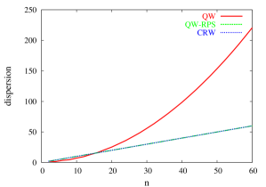
Figure 1: (Color online) Dispersions of the probability distributions corresponding to the $n$ steps of quantum walk (solid/red line), the (memoryless) classical random walk with equal probabilities of step in any direction (dotted/blue line), and the quantum walk with random phase shifts (dashed/green line) for a two-dimensional system. The initial state of the quantum system system is described by a vector $|\psi_{0}\rangle=|0\rangle\otimes|s\rangle$ and we assume the Grover coin $C_{G}$. The quantities for QW-RPS were obtained by generating 50 evolutions of QW-RPS with respective dispersions of probability distributions, and by averaging over them.

Comparing the three corresponding lines we find that the dispersion in the QW grows quadratically with number of steps meyer1996 (see solid/red line in Fig. 1). This is in a sharp contrast to a classical random walk for which the dispersion is a linear function of the number of steps (see dotted/blue line in Fig. 1). The lines for QW-RPS and CRW overlap. The dispersion of either grows linearly with the number of steps $n$ (see dashed/blue line in Fig. 1).

In Fig. 2 we plot the dispersion (40) as a function of number of steps for a three-dimensional ($d=3$) QW, CRW and QW-RPS, respectively.

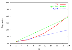
Figure 2: (Color online) Dispersions of probability distributions corresponding to the $n$ steps of quantum walk (solid/red line), the (memoryless) classical random walk with equal probabilities of step in any direction (dotted/blue line), and the quantum walk with random phase shifts (dashed/green line) for a three-dimensional system. The initial state of the quantum system system is described by a vector $|\psi_{0}\rangle=|0\rangle\otimes|s\rangle$ and we assume the Grover coin $C_{G}$. The quantities for QW-RPS were obtained by generating 50 evolutions of QW-RPS with respective dispersions of probability distributions, and by averaging over them.

As in the two-dimensional case, the dispersion of the probability distribution of the QW grows quadratically. The dispersion of the classical random walk is a linear function of number of steps and it does not depend on the dimension of the random walk. Interestingly enough, the dispersion of the quantum walk with random phase shifts is again a linear function, but unlike in the two-dimensional case, for $d\geq 3$ the linear growth of the dispersion is faster than in the classical case.

The same conclusions can be derived from our simulations of quantum walks in four-dimensional space (see Fig. 3).

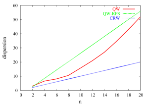
Figure 3: (Color online) Dispersions of probability distributions corresponding to $n$ steps of quantum walk (solid/red line), the (memoryless) classical random walk with equal probability of step in any direction (dotted/blue line), and the quantum walk with random phase shifts ($\mathcal{D}_{0}(D,n)$: dashed/green line) for a four-dimensional system. The initial state of the quantum system is described by a vector $|\psi_{0}\rangle=|0\rangle\otimes|s\rangle$. We assume the Grover coin $C_{G}$.The quantities for QW-RPS were obtained by generating 50 evolutions of QW-RPS with respective dispersions of probability distributions, and by averaging over them.

In Fig. 4 we plot dispersion of probability distributions for quantum walks with random phase shifts as a number of steps for various dimensions $d=2,3,4$. We generated 50 evolutions of QW-RPS for each dimension, and averaged over the respective dispersion generated by each evolution.

We can conclude, that as the dimension increases, the linear growth of the dispersion also increases.

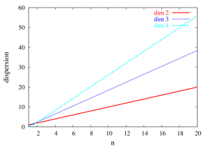
Figure 4: (Color online) Dispersion of QW-RPS processes for different dimensions for $n$ steps. We see that these dispersions $\mathcal{D}_{0}(D,n)$ are linear functions with gradients that depend on the dimensionality of the system under consideration. Only the case $d=2$ coincides with the classical random walk. The quantities for QW-RPS were obtained by generating 50 evolutions of QW-RPS with respective dispersions of probability distributions, and by averaging over them.

We have shown that the introduction of random phase shifts causes the transition of a QW to a (quasi-)classical random walk. In our previous discussion we have considered random phases to be uniformly distributed in the interval $[-\pi,\pi]$. Here we briefly analyze a situation when phases of random shifts are distributed according to a normal distribution that is peaked around the phase zero and with the dispersion $\sigma$. When the dispersion is zero, (i.e. $\sigma=0$) we recover the QW (see Fig. 5), while for large $\sigma$, we obtain uniform distribution on the interval $[-\pi,\pi]$ and the CRW is obtained. The results are shown in Fig. 5. This analysis clearly shows the quantum-to-classical transition for quantum walks which is generated by random phase shifts. As the phase shifts become more random, the walk becomes more classical.

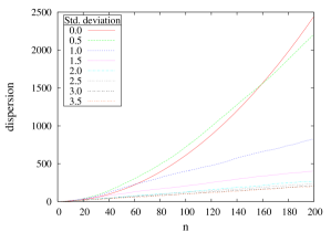
Figure 5: (Color online) Dispersion $\mathcal{D}_{0}(D,n)$ of $n$ steps of QW-RPS in dimension 2 with random phases normally distributed around 0 with respective standard deviation. We see a “continuous” transition between the QW and CRW as function of the standard deviation of the random phase distribution.

IV Conclusion

We have shown that by shifting the amplitudes of the coin register in a quantum walk by random phases, we can obtain the classical behavior of the quantum walk. For a Grover coin, the mean probability distribution of such a walk is equivalent to the CRW with memory and a biased coin; for the Fourier coin, the mean probability distribution is equivalent to the memoryless CRW with an unbiased coin (given an unsymmetric initial coin state).

The results underlying Fig. 5 also show how the transition from QW-RPS to CRW occurs when we increase the dispersion of the normal distribution of random phases (for the Grover coin). Our results are in a way complementary to a standard quantization procedure in physics. Specifically, classical dynamics of physical systems can be canonically quantized, so it is clear what is the quantum version of a classical process. On the other hand, quantum walk is not obtained by a canonical quantization procedure from a classical random walk. It is simply defined by a set of instructions that govern the evolution of the quantum walk. Therefore it is of importance to know what is the underlying classical process. This underlying process can be reconstructed either by measuring the coin at each step (cf. AAKV01a ), or when the quantum walk is subject to random phase shifts that totally suppress quantum interference between different evolution paths. As a result of the suppression of the quantum interference, the classical random walk that corresponds to the underlying quantum walk emerges.

Appendix A Dispersion of QW-RPS with Grover coin

Starting with Eq. (39) we can evaluate the dispersion $\mathcal{D}(D,n)$ of QW-RPS with generalized Grover coin $G_{r,t}$. The dispersion reads

$$\mathcal{D}(D,n)=K\sum_{\mathbf{a}\in D^{n}}|\mathbf{e}_{a_{1}}+\dots+\mathbf{e}_{a_{n}}|^{2}|\;\Xi(\mathbf{a})|^{2}$$ (54)

with $K=\left|\frac{r-t}{\sqrt{|D|}}+\sqrt{|D|}t\right|^{2}$. Turning Eq. (54) into the recursive relation we obtain

$$\begin{split}\mathcal{D}(D,n)&=K\sum_{\mathbf{a}\in D^{n+1}}\Big{\{}|\mathbf{e}_{a_{1}}+\dots+\mathbf{e}_{a_{n}}|^{2}\\ &+2(\mathbf{e}_{a_{1}}+\dots+\mathbf{e}_{a_{n}})\cdot\mathbf{e}_{a_{n+1}}+1\Big{\}}\\ &\times|\Xi(a_{1},\dots,a_{n})|^{2}\;|\Xi(a_{n},a_{n+1})|^{2}\;.\end{split}$$ (55)

We find that $\sum_{a_{n+1}\in D}|\Xi(a_{n},a_{n+1})|^{2}=|r|^{2}+(|D|-1)|t|^{2}=1$ for all $a_{n}\in D$. Hence the first and the last terms in the braces contribute to Eq. (55) with $\mathcal{D}(D,n)+1$. The middle term has the form

$$2K\sum_{\mathbf{a}\in D^{n}}|\Xi(\mathbf{a})|^{2}\,(\mathbf{e}_{a_{1}}+\dots+\mathbf{e}_{a_{n}})\cdot\sum_{a_{n+1}\in D}|\Xi(a_{n},a_{n+1})|^{2}\mathbf{e}_{a_{n+1}}\;.$$ (56)

In the sum over $a_{n+1}$ in Eq. (56), we can keep just the terms $a_{n+1}$ such that $\mathbf{e}_{a_{n+1}}$ is parallel with $\mathbf{e}_{a_{1}}+\dots+\mathbf{e}_{a_{n}}$. The remaining $a_{n+1}$-s cancel out, since for each such $a_{n+1}$ there is $a_{n+1}^{\prime}$ such that $\mathbf{e}_{a_{n+1}}+\mathbf{e}_{a_{n+1}}^{\prime}=0$. Hence the second term of Eq. (56) can be rewritten as

$$\begin{split}2K&(|r|^{2}-|t|^{2})\sum_{\mathbf{a}\in D^{n}}|\Xi(\mathbf{a})|^{2}\,(\mathbf{e}_{a_{1}}+\dots+\mathbf{e}_{a_{n}})\cdot\mathbf{e}_{a_{n}}\\ &\equiv 2K(|r|^{2}-|t|^{2})R_{n}\;.\end{split}$$ (57)

The expression for $\mathcal{D}(D,n)$ reads as

$$\mathcal{D}(D,n+1)=\mathcal{D}(D,n)+1+2K(|r|^{2}-|t|^{2})R_{n}$$ (58)

with

$$\begin{split}\mathcal{D}(D,2)&=K\sum_{a_{1},a_{2}\in D}|\Xi(a_{1},a_{2})|^{2}|a_{1}+a_{2}|^{2}\\ &=K\big{\{}4|D|\,|r|^{2}+2(|D|^{2}-|D|-1)|t|^{2}\big{\}}\;.\end{split}$$ (59)

The expression $R_{n}$ can be rewritten into recursive equation:

$$R_{n+1}=(|r|^{2}-|t|^{2})R_{n}+\frac{1}{K}$$ (60)

with the initial condition

$$\begin{split}R_{2}&=\sum_{a_{1},a_{2}\in D}|\Xi(a_{1},a_{2})|^{2}(\mathbf{e}_{a_{1}}+\mathbf{e}_{a_{2}})\cdot\mathbf{e}_{a_{2}}\\ &=2|D||r|^{2}+(|D|^{2}-|D|-1)|t|^{2}\;.\end{split}$$ (61)

Eqs. (60) and (61) can be solved to obtain

$$\begin{split}R_{n}&=\frac{(|r|^{2}-|t|^{2})^{n-2}(KR_{2}|r|^{2}-KR_{2}|t|^{2}-KR_{2}+1)-1}{K(|r|^{2}-|t|^{2}-1)}\;.\end{split}$$ (62)

Solving Eq. (58) and collecting the terms from Eqs. (59), (61), and (62) we obtain

$$\begin{split}\mathcal{D}&(D,n)=\frac{1}{(|r|^{2}-|t|^{2})(1-|r|^{2}+|t|^{2})^{2}}\times\\ &\times\Big{\{}(n-2)\xi-2(|r|^{4}+|t|^{4})+4|r|^{2}\,|t|^{2}+\\ &+(2+\eta)(|r|^{2}-|t|^{2})^{n}+\eta\big{[}|t|^{2}-|r|^{2}\big{]}\Big{\}}\;,\end{split}$$ (63)

where

$$\begin{split}\xi&=|r|^{2}-|r|^{6}-|t|^{2}+3|r|^{4}|t|^{2}-3|r|^{2}|t|^{4}+|t|^{6}\;{}^{\prime}\end{split}$$ (64)

and

$$\begin{split}\eta&=2\Big{|}\frac{r+(|D|-1)t}{\sqrt{|D|}}\Big{|}(|r|^{2}-|t|^{2}-1)\\ &\times\Big{\{}2|D||r|^{2}+(|D|^{2}-|D|-1)|t|^{2}\Big{\}}\;.\end{split}$$ (65)

We may assume that $r$ is real and $t=|t|e^{i\alpha}$. Solving Eqs. (23) and (24) we obtain

$$|t| = \left(\frac{1-r^{2}}{|D|-1}\right)^{1/2}\;;$$ (66)

$$\alpha = \pm\arccos\left[\frac{1}{2r}(2-|D|)\left(\frac{1-r^{2}}{|D|-1}\right)^{1/2}\right]\;,$$ (67)

where $|D|\geq 4,\,\frac{|D|-2}{|D|}\leq r<1$. Obviously, $0\leq|r|,|t|\leq 1$ and $|r|^{2}-|t|^{2}=\frac{|D|r^{2}-1}{|D|-1}$. Eq. (63) contains only two terms dependent on $n$: $(n-2)\xi$ and $(|r|^{2}-|t|^{2})^{n}$. The latter goes to 0 as $n\rightarrow\infty$, hence we get ($n>2$):

$$\mathcal{D}(D,n)=\frac{1+|r|^{2}-|t|^{2}}{1-|r|^{2}+|t|^{2}}(n-2)+O\Big{(}(|r|^{2}-|t|^{2})^{n}\Big{)}\;.$$ (68)

References

• (1) Y. Aharonov, L. Davidovich, and N. Zagury: Quantum random walks, Phys. Rev. A 48, 1687 (1993)
• (2) N. Shenvi, J. Kempe, and K.B. Whaley: Quantum random-walk search algorithm, Phys. Rev. A 67, 052307 (2003)
• (3) A.M. Childs and J.M. Eisenberg: Quantum algorithm for subset finding, Quantum Inf. & Comp. 5, 593 (2005).
• (4) M. Szegedy: Spectra of Quantized walks and a $\sqrt{\epsilon\delta}$-rule, quant-ph/0401053 (2004)
• (5) J. Kempe: Quantum random walks: An introductory overview, Contemp. Phys. 44, 307-327 (2003).
• (6) D. Aharonov, A. Ambainis, J. Kempe, and U. Vazirani: Quantum walks on graphs, Proc. 33th STOC, pp. 50-59 (2001)
• (7) A. Ambainis, E. Bach, A. Nayak, A. Vishwanath, and J. Watrous: One-dimensional quantum walks, Proc. 33th STOC, pp. 60-69 (2001)
• (8) V. Kendon and B. Tregenna: Decoherence in a quantum walk on a line In: J.H. Shapiro and O. Hirota (Eds.), Quantum Communication, Measurement & Computing - QCMC 02 (Rinton Press, 2002), p. 463.
• (9) V. Kendon and B. Tregenna: Decoherence can be useful in quantum walks, Phys. Rev. A 67, 042315 (2003).
• (10) T.A. Brun, H.A. Carteret, and A. Ambainis: Quantum walks driven by many coins, Phys. Rev. A 67, 052317 (2003)
• (11) T. A. Brun, H.A. Carteret, and A. Ambainis: The quantum to classical transition for random walks, Phys. Rev. Lett. 91, 130602 (2003)
• (12) C. Moore and A. Russell: Quantum walks on the hypercube, Proc. RANDOM 2002, pp. 164-178 (2002)
• (13) D.A. Meyer: From quantum cellular automata to quantum lattice gasses, J. Stat. Phys. 85, 551 (1996)