Performance of Deterministic Dynamical Decoupling Schemes: Concatenated and Periodic Pulse Sequences

Abstract

Dynamical decoupling can be used to preserve arbitrary quantum states despite undesired interactions with the environment, using control Hamiltonians affecting the system only. We present a system-independent analysis of dynamical decoupling based on leading order decoupling error estimates, valid for bounded-strength environments. Using as a key tool a renormalization transformation of the effective system-bath coupling Hamiltonian, we delineate the reliability domain of dynamical decoupling used for quantum state preservation, in a general setting for a single qubit. We specifically analyze and compare two deterministic dynamical decoupling schemes – periodic and concatenated – and distinguish between two limiting cases of fast versus slow environments. We prove that concatenated decoupling outperforms periodic decoupling over a wide range of parameters. These results are obtained for both “ideal” (zero-width) and realistic (finite-width) pulses This work extends and generalizes our earlier work, Phys. Rev. Lett. 95, 180501 (2005).

I Introduction

Arbitrary quantum state preservation is a fundamental imperative for quantum information processing, but undesired interactions of a candidate quantum system with uncontrollable external systems (the environment/bath) results in poor control and fidelity loss. Even if the structure of these interactions is approximately known, the statistical uncertainty in the state of the environment invariably results in decoherence Zurek . While undesired couplings to the environment are inevitable (even at zero temperature), strong control fields applied to the system can be used to effectively manipulate the couplings. Nuclear magnetic resonance is an excellent example where techniques such as refocusing and composite pulses are readily used to generate reliable and high precision quantum dynamics Freeman:book ; vandersypen:04 . Similar in execution but applicable in a generic setting, dynamical decoupling (DD) is a method for the effective renormalization of the system-bath interaction Hamiltonian via the application of strong system-control fields. Usually the goal is the cancellation of all coupling terms. In the context of quantum information processing, DD can be used for feedback-free quantum error suppression without encoding overhead Viola:99 .

Dynamical decoupling is most efficient against bounded environments, when the pulse switching times are short on a scale set by the bath spectral density high-frequency cutoff Viola:98 ; Facchi:05 , or when the spectral density is rapidly decaying ShiokawaLidar:02 . Within these assumptions different flavors of DD can be designed. Of course, technology limits how strongly, rapidly and accurately we can modulate the system Hamiltonian, and cool the system. Dynamical decoupling can be implemented with the pulse sequence chosen deterministically, e.g., periodically Viola:98 ; ByrdLidar:01 ; pryadko:085321 , or randomly Facchi:03 ; Viola:05 . Randomized decoupling is expected to perform better in the case of varying/fluctuating (effective) Hamiltonians while deterministic methods perform better in cases where the undesired terms in the system-bath Hamiltonian are sufficiently weak Santos:06 ; Viola:06 . Hybrid schemes with optimized performance have also been considered Viola:05 ; kern:250501 . The analysis of DD schemes is often performed within an interaction picture. Here we consider explicitly the internal dynamics of the bath in terms of its effect on the performance of DD.

Dynamical decoupling strategies, some of which can be derived from group theoretical considerations Zanardi:98b , are typically based on a universal DD pulse sequence Viola:99 : a short sequence of unitary operators designed to completely cancel errors up to the first order in the Magnus expansion Magnus:54 . Here we consider two deterministic decoupling schemes: (i) In periodic DD (PDD), the universal decoupling sequence is repeated periodically for the duration of the quantum state preservation. (ii) In concatenated dynamical decoupling (CDD) KhodjastehLidar:04 , the universal pulse sequence is recursively embedded within itself. We provide an analytic leading-order study of the performance of the above strategies. Our first basic finding is a verification in the DD-setting of a result familiar from NMR, that even when ideal (zero-width) pulses are used for decoupling, the corrections from second and higher order Magnus terms impose an upper performance bound on PDD.

A central result of our approach is that the coupling terms responsible for errors undergo an effective renormalization transformation by the externally applied pulse sequences. This process is conveniently described via the Magnus expansions for derivation of effective coupling Hamiltonians [see Eqs. (41)-(44) below]. The renormalization approach leads to the view of DD as a dynamical map, whose convergence to a fixed point (ideally, the cancellation of the system-bath interaction) depends on whether the norm of the coupling terms decreases under repeated applications of the pulse sequence. In support of our earlier study KhodjastehLidar:04 , within the technological constraints of finite pulse numbers and the bounds imposed by the applicability of DD in general, we analytically prove the asymptotic superiority of CDD over PDD. In addition, we present here new pulse sequences, inspired by the Trotter-Suzuki expansion Suzuki:76 , with even better convergence properties than CDD. In a more abstract setting, we show that in fact any application of unitary operators on the system cannot cause an increase in the strength of the undesired couplings.

Our conclusions are valid within the convergence domain of our expansions. We find that the Magnus expansion itself sets the most stringent limit on convergence domains, in the sense that it includes or coincides with the regime of applicability of DD. In the worst case, this corresponds to the limit of slow internal bath dynamics.

We also analyze robustness with respect to systematic pulse errors. The decoupling error of any deterministic scheme is thus a result of the environmental coupling errors, and errors in the decoupling operations. In the case of realistic, imperfect pulses, we show that the performance of DD, when pulses of finite width (or uniform error rate) are used, is determined by a condition based on both the pulse switching times and pulse widths. In this case, unless pulse profiles and timings are adjusted in case of systematic pulse errors, even the first order terms (and thus dominating) in the Magnus expansion will be non-zero.

While undesired coupling terms are responsible for fidelity loss, the relationship between the two is complicated and depends on the details of the environment and possible physical energy cutoffs. This motivates us to perform a generic analysis based on operator-norm estimates. Our conservative estimates provide a worst-case analysis for decoupling performance. We expect these estimates to be useful as guidelines for choosing and combining dynamical decoupling strategies when constraints such as pulse switching times and pulse errors are considered.

This paper is organized as follows: in Section II we review the basic universal DD cycle which suffices to decouple a qubit from an arbitrary non-Markovian environment to first order in the Magnus expansion. In Section III we provide a detailed analysis of this sequence in terms of the Magnus expansion, for both ideal (zero-width) and non-ideal (finite-width) pulses. In Section IV we compare two deterministic decoupling strategies founded on the basic universal DD sequence: periodic and concatenated sequences. We calculate a fidelity measure associated with the two strategies and show that the concatenated one strictly outperforms the periodic one. In Section V we introduce a new decoupling strategy, based on the Trotter-Suzuki expansion. Even though this decoupling sequence has implementations problems and is not as robust as CDD, we find it interesting in light of its superior convergence properties. This Section also includes a table which compares the three deterministic decoupling strategies (PDD, CDD, and Trotter-Suzuki), and clearly illustrates and summarizes their relative performance. Finally, in Section VI we present a general result concerning the behavior of error norms under pulse sequences: we show that for sufficiently narrow pulses, pulse sequences cannot increase error norms. This result has impact also on fault tolerance theory using quantum error correcting codes. A summary and discussion is presented in Section VII. Supporting calculations can be found in the Appendices.

II Universal Dynamical Decoupling for a Qubit

In the absence of driving terms, the terms in the system-bath interaction Hamiltonian are responsible for decoherence and loss of quantum information. Removal of these terms is sufficient (but not necessary LidarWhaley:03 ) for preservation of arbitrary quantum states. Dynamical decoupling schemes use strong and fast control Hamiltonians acting on the quantum system only, to effectively remove/modify various terms in the system-bath interaction Hamiltonian CDD-PRA:note1 . In particular, a pulse sequence designed to remove every term in the interaction Hamiltonian is referred to as universal dynamical decoupling. In this work, we focus on the universal DD of a single qubit. Extensions to multiple qubits Viola:99 and higher dimensional quantum systems exist WuByrdLidar:02 ; ByrdLidarWuZanardi:05 , but we will not consider these here. We use $X$, $Y$, and $Z$ to denote the standard $2\times 2$ Pauli matrices

$$\sigma_{x}=\begin{pmatrix}0&1\\ 1&0\end{pmatrix},\,\sigma_{y}=\begin{pmatrix}0&-i\\ i&0\end{pmatrix},\,\sigma_{z}=\begin{pmatrix}1&0\\ 0&-1\end{pmatrix}$$

acting on a single qubit, and work in units of $\hbar=1$. System and environment are assumed to inhabit different Hilbert spaces i.e., we do not consider leakage, which can also be treated using DD WuByrdLidar:02 ; ByrdLidarWuZanardi:05 ), and all Hamiltonian operators are taken to be traceless without loss of generality.

Consider a qubit with a Hamiltonian

$$H(t)=H_{\text{ctrl}}(t)+H_{e}(t),$$ (1)

where $H_{\text{ctrl}}$ refers to a time-dependent controllable system-only part and $H_{e}$ includes all other terms, i.e., the internal bath, internal system, and interaction Hamiltonians:

$$H_{e}=H_{B}\otimes I_{S}+I_{B}\otimes H_{S}+H_{SB}.$$ (2)

Here $I$ denotes the identity operator. We have implicitly excluded a pure-bath Hamiltonian term $H_{B}^{0}\otimes I_{S}$ satisfying $[H_{B}^{0}\otimes I_{S},F]=0$, where $F$ is any element of the Lie algebra generated by $H_{SB}$, $H_{B}\otimes I_{S}$, and $I_{B}\otimes H_{S}$. The reason is that such a term on the one hand does not impact the system dynamics, but on the other hand will increase the operator norm that arises below in our calculations of decoupling errors. With this in mind, ideally one would like to have $H_{e}=0$. The “error Hamiltonian” $H_{e}$ can always be expanded as:

$$H_{e}=B_{0}\otimes I_{S}+B_{X}\otimes X+B_{Y}\otimes Y+B_{Z}\otimes Z$$ (3)

where $B_{\alpha}$ ($\alpha=0,X,Y,Z$) are operators acting on the environment. We are allowing the $B_{\alpha}$ to include the identity operator, i.e., from now on we are incorporating $H_{S}$ into $H_{SB}$. I.e., assuming

$$H_{S}=\sum_{\alpha=x,y,z}\omega_{\alpha}\sigma_{\alpha},$$ (4)

with $\omega_{\alpha}$ all non-zero frequencies, and writing

$$H_{SB}=\sum_{\alpha=x,y,z}b_{\alpha}\otimes\sigma_{\alpha},$$ (5)

yields

$$B_{\alpha} = \omega_{\alpha}I_{B}+b_{\alpha}\quad\alpha\in\{x,y,z\},$$

$$B_{0} = I_{B}+H_{B}.$$ (6)

Note that the first term in $H_{e}$, $B_{0}\otimes I_{S}$, is a pure-environment term and simply generates the environment’s internal dynamics. It also includes the global phase generating term $I_{B}\otimes I_{S}$. Obviously if $b_{X}=b_{Y}=b_{Z}=0$, then $H_{e}=B_{0}\otimes I_{S}$ has no effect on the system dynamics.

Universal DD of a qubit with ideal pulses removes every term in $H_{e}$ except $B_{0}\otimes I_{S}$, by applying the following pulse sequence: f$X$f$Z$f$X$f$Z$, where $\mathtt{f}$ denotes a “pulse-free” period of fixed duration. The pulses are generated by $H_{\text{ctrl}}$. This universal DD sequence is a simplification of $(I_{S}\mathtt{f}I_{S})(X\mathtt{f}X)(Y\mathtt{f}Y)(Z\mathtt{f}Z)$, where $X,Y,Z$ and the identity $I_{S}$ represent the decoupling group ${\mathcal{G}}$ on the qubit. The universal decoupling group has the property that for every Hamiltonian $H$ acting on the system, the sum $\sum_{\{P_{i}\in{\mathcal{G}}\}}P_{i}HP_{i}^{{\dagger}}$ acts trivially on the system Viola:99 . Since this sum is the leading order generator in the Magnus expansion, the universal DD sequence completely removes any system-bath interaction to first order (we revisit this in detail in subsection III.2).

A complete analysis of the performance of DD needs to take into account details of the environment (participating modes, energy cutoffs, temperature, (dis)equilibrium, etc.) but we shall minimize these considerations and focus on the model-independent features of DD. Our analysis is mathematically constrained by convergence domains that are explicit in our approximations. We expect certain unbounded systems such as bosonic environments to be within the realm of our theoretical framework after the introduction of spectral cutoffs.

III Analysis of the Universal Decoupling Pulse Sequence: The Renormalization Transformation

In this section we derive the transformation of various Hamiltonian terms under the basic universal DD pulse sequence. We first consider ideal pulses, then amend our discussion to allow for non-ideal (finite width) pulses. We will see that the system-bath interaction Hamiltonian is effectively renormalized under the DD pulse sequence. As long as this renormalization transformation is norm-reducing, the DD procedure is effective.

III.1 Ideal Pulses

Let us first assume that the pulses used are ideal, i.e., infinitely strong and narrow. For example, $H_{\text{ctrl}}(t)=\frac{\pi}{2}\delta(t-t_{0})X$ generates an ideal $X$ pulse at time $t_{0}$ ($\delta$ is the Dirac $\delta$-function). The propagator corresponding to free evolution $\mathtt{f}$ of period $\tau_{0}$ is given by:

$$U_{\mathtt{f}}=\exp(-i\tau_{0}H^{(0)}),\quad H^{(0)}:=H_{e}.$$ (7)

To obtain the cycle propagator we use the identity $Me^{A}M^{-1}=e^{MAM^{-1}}$, valid for any operator $A$ and invertible $M$. Define

$$H_{1} \equiv B_{0}\otimes I+B_{X}\otimes X+B_{Y}\otimes Y+B_{Z}\otimes Z=IH_{e}I,$$

$$H_{2} \equiv B_{0}\otimes I+B_{X}\otimes X-B_{Y}\otimes Y-B_{Z}\otimes Z=XH_{e}X,$$

$$H_{3} \equiv B_{0}\otimes I-B_{X}\otimes X+B_{Y}\otimes Y-B_{Z}\otimes Z=YH_{e}Y,$$

$$H_{4} \equiv B_{0}\otimes I-B_{X}\otimes X-B_{Y}\otimes Y+B_{Z}\otimes Z=ZH_{e}Z,$$ (8)

The free evolution propagator can then also be written as f$=\exp(-i\tau_{0}H_{1})$. Using Eqs. (8) we can write the total propagator corresponding to the universal DD cycle, $(I\mathtt{f}I)(X\mathtt{f}X)(Y\mathtt{f}Y)(Z\mathtt{f}Z)$, in terms of four effective Hamiltonians describing the different evolution segments, as:

$$U_{1}=e^{-i\tau_{0}H_{1}}e^{-i\tau_{0}H_{2}}e^{-i\tau_{0}H_{3}}e^{-i\tau_{0}H_{4}}.$$ (9)

A time-varying piecewise constant Hamiltonian, $H(t)$ varying over four intervals each of length $\tau_{0}$, can generate this propagator. The total propagator can then be used to define the effective Hamiltonian $H^{(1)}$:

$$U_{1}=\prod_{i=1}^{4}\exp(-i\tau_{0}H_{i}^{(0)})=:\exp(-i4\tau_{0}H^{(1)}),$$ (10)

where we have added superscripts $(0)$ to the Hamiltonians $H_{i}$ of Eq. (8), in anticipation of the concatenation procedure that we consider in subsection IV.3.

III.2 Magnus Expansion

The cycle propagator $U_{1}$ [Eq. (10)] can be approximated using a Magnus expansion (for an alternative method of analysis that is particularly useful for the design of periodic sequences of soft pulses see Ref. sengupta:037202 ). Consider a time-dependent Hamiltonian $H(t)$ generating the propagator $U(t)$ from time $0$ to $t$. In the Magnus expansion (a type of cumulant expansion) we have

$$U(t)=\exp\sum_{i=1}^{\infty}A_{i}(t),$$ (11)

with $A_{1}$ and $A_{2}$ given by:

$$A_{1} =-i\int_{0}^{t}dt_{1}H(t_{1}),$$ (12)

$$A_{2} =-\frac{1}{2}\int_{0}^{t}dt_{1}\int_{0}^{t_{1}}dt_{2}[H(t_{1}),H(t_{2})].$$ (13)

Higher order terms are given by higher order commutator expressions Magnus:54 . A recent bound for the convergence radius of the Magnus expansion Moan:01 translates in our case into $\max{\|H(t)\|}t<2$. In many situations $\|B_{0}\|$ (norm of the environment’s internal Hamiltonian) is expected to dominate the Hamiltonian and we may as well use $\|B_{0}\|t\lesssim 1$ as a conservative convergence domain. This bound can, however, be superficial since not all degrees of freedom of the environment might actually be involved in the dynamics. For example, in a spin bath, bath spins far away from the system will not immediately contribute to the dynamics but this will nonetheless increase $\|B_{0}\|$ without changing the real convergence radius. A precise analysis of the actual convergence radius requires us to estimate the next-to-leading-order terms – see Appendix A.

For the piecewise constant evolution of the Hamiltonian in Eq. (9), we can calculate $A_{1}$ and $A_{2}$ in terms of $H(t)=$ $\{H_{j}$ for $(j-1)\tau_{0}\leq t\leq j\tau_{0}\}_{j=1}^{4}$, i.e., the sign-flipped Hamiltonians appearing in Eq. (9):

$$A_{1}^{(1)} =-i\tau_{0}(H_{1}^{(0)}+H_{2}^{(0)}+H_{3}^{(0)}+H_{4}^{(0)})$$ (14)

$$A_{2}^{(1)} =-\frac{1}{2}\tau_{0}^{2}\sum_{1=i<j=4}[H_{i}^{(0)},H_{j}^{(0)}].$$ (15)

Again, the superscripts are included in anticipation of the CDD analysis below. Note that the pure-environment parts of $A_{i}^{(1)}$, i.e., terms of the form $B\otimes I$, have no effect on the dynamics of the qubit to first order in $\tau_{0}$, but do have an effect to second order in $\tau_{0}$, through the commutator terms. Clearly, pure-environment terms are not renormalized under the DD procedure.

Using Eqs. (8),(14),(15) we find:

$$A_{1}^{(1)} = -i(4\tau_{0})B_{0}\otimes I$$

$$A_{2}^{(1)} = 4\tau_{0}^{2}[B_{0},B_{X}]\otimes X$$ (16)

$$+2\tau_{0}^{2}\left([B_{0},B_{x}]-i\{B_{X},B_{Z}\}\right)\otimes Y$$

This shows that while to first order in the Magnus expansion (the $A_{1}^{(1)}$ term) the universal decoupling cycle completely removes the coupling to the environment, there is a leading second order correction due to $A_{2}^{(1)}$ in which the coupling to the environment has not been removed.

Note that a pure-environment term appears only in $A_{1}^{(1)}$ and, due to our particular choice of DD sequence, f$X$f$Z$f$X$f$Z$, there is no term involving $\otimes Z$ in $A_{2}^{(1)}$.

We now define two norms which will play a central role in our analysis:

$$\beta :=\left\|B_{0}\right\|<\infty$$ (17)

$$J :=\max(\left\|B_{X}\right\|,\left\|B_{Y}\right\|,\left\|B_{Z}\right\|)<\infty.$$ (18)

Recall that $B_{\alpha}=\omega_{\alpha}I_{B}+b_{\alpha}$ for $\alpha\in\{x,y,z\}$, and $B_{0}=I_{B}+H_{B}$; unless otherwise specified, we assume that $J<\beta$ in order to simplify our convergence arguments. This conservative assumption is reasonable for systems where only a small number of environment particles (or degrees of freedom) are coupled to a given qubit (such as electron spins coupled to a nuclear spin bath khaetskii:186802 ) – which translates into a small $\|b_{\alpha}\|$ – whereas no restriction exists on the environment self-Hamiltonian (e.g., on the number of particles). The distinction between $J$ and $\beta$ is a reflection of the different roles $H_{SB}$ and $H_{B}$ play in the dynamics of the system. In simple terms, $J$ quantifies the direct coupling strength while $\beta$ quantifies typical bath frequencies. Consider, e.g., the simple case of a spin qubit coupled to another spin-$1/2$ particle via a Heisenberg coupling: $H_{e}=\omega Z_{B}\otimes I+c(X_{B}\otimes X+Y_{B}\otimes Y+Z_{B}\otimes Z)$, where $c$ is the coupling coefficient. In this case we have: $J=O(c)$ and $\beta=O(\omega)$.

The Magnus terms can be bounded using these quantities: $\|A_{1}^{(1)}\|=O(\tau_{0}\beta)$ and $\|A_{2}^{(1)}\|=O(\tau^{2}_{0}\beta J)$. Higher order Magnus terms, $A_{i>2}^{(1)}$, will contain all orders of $\tau_{0}^{i}J^{k}\beta^{i-k}$ where $1\leq k\leq i-1$, and the leading term is always given by $O(\tau_{0}^{i}J\beta^{i-1})$ since $J<\beta$. As long as $\tau_{0}\beta\ll 1$ we can safely neglect $A_{i>2}^{(1)}$:

$$||A_{i>2}^{(1)}||\ll||A_{2}^{(1)}||<||A_{1}^{(1)}||\text{.}$$ (19)

Note that our derivations are based on the separation of the coupling terms $B_{0}\otimes I$ and $B_{X}\otimes X+B_{Y}\otimes Y+B_{Z}\otimes Z$ in the error Hamiltonian $H_{e}$. A similar separation can be done for decoupling schemes on systems other than a single qubit.

The approximate effective Hamiltonian $H^{(1)}$ corresponding to the basic dynamical decoupling cycle, Eq. (10), is now:

$$H^{(1)}\approx\frac{1}{-i4\tau_{0}}(A_{1}^{(1)}+A_{2}^{(1)}):=\sum_{\alpha}B_{\alpha}^{(1)}\otimes\sigma_{\alpha}.$$ (20)

The renormalized environment operators $B_{\alpha}^{(1)}$, which can easily be read off from Eqs. (16), are the main result of the DD procedure. The important message emerging from the analysis in this subsection is that even when ideal (infinitely strong and narrow) pulses are used, the universal decoupling cycle only removes (the system-bath component of) the lowest order Magnus term, and renormalizes the higher order Magnus terms. The success of dynamical decoupling ultimately depends on whether the mapping to the renormalized environment operators is significantly norm-decreasing, an issue we address in detail below.

III.3 Pulses of Finite Width

Ideal pulses that act as system-only unitary operators are simplified mathematical abstractions. In this subsection we model and analyze the effect of the finite width of pulses in decoupling. For simplicity we consider rectangular pulses $P$ with a width $\delta$. The ideal finite-width pulse is,

$$P=\exp(-i\delta H_{P}),$$ (21)

where $H_{P}$ is a fixed control Hamiltonian. For realistic pulses we must include $H_{e}$ in the pulse propagator:

$$U_{P}=\exp(-i\delta(H_{P}+H_{e})).$$ (22)

We call such a pulse “non-ideal”. Extremely narrow pulses with $||H_{P}||\gg||H_{e}||$ are thus desirable to minimize the effect of the unwanted terms in the pulse Hamiltonian. Here we build upon the approximation of instantaneous pulses in subsection III.2, by decomposing the non-ideal pulses into products of the ideal unitary operator of the pulse $P$ and some effective pulse error unitary operator $E_{P}$. We explicitly approximate the operators $E_{P}$ for rectangular pulses on a qubit, but the decomposition of the actual pulse into an ideal pulse and a “pulse error” unitary can be reproduced for other pulse shapes as well.

The periods of the universal dynamical decoupling cycle need to be adjusted in order to incorporate the time delays associated with finite pulse widths. Therefore, assume that all free evolution periods, with propagator $U_{\mathtt{f}}$, are adjusted to length $\tau_{0}-\delta$. The propagator for the cycle can then be written as:

$$U^{(1)} =U_{\mathtt{f}}U_{X}U_{\mathtt{f}}U_{Z}U_{\mathtt{f}}U_{X}U_{\mathtt{f}}U_{Z}$$

$$=U_{\mathtt{f}}E_{X}XU_{\mathtt{f}}XE_{Z}^{\prime}YU_{\mathtt{f}}YE_{X}^{\prime}ZU_{\mathtt{f}}ZE_{Z}$$

$$=:U_{\mathtt{f}_{1}}E_{X}U_{\mathtt{f}_{2}}E_{Z}^{\prime}U_{\mathtt{f}_{3}}E_{X}^{\prime}U_{\mathtt{f}_{4}}E_{Z}$$ (23)

where

$$U_{\alpha}=e^{-i\delta(\eta\sigma_{\alpha}+H_{e})}\qquad\alpha=X,Z,$$ (24)

$\delta\eta=\pi/2$, and, in order to fit the formulation of subsection III.2, we have defined the pulse-error operators as follows:

$$E_{X}X:=U_{X}, \hskip 28.45274ptYE_{X}^{\prime}Z:=U_{X},$$ (25)

$$ZE_{Z}:=U_{Z}, \hskip 28.45274ptXE_{Z}^{\prime}Y:=U_{Z}.$$ (26)

Note that since the errors $E_{\alpha}$ are unitary and are produced during an interval $\delta$, we may formally associate them with effective Hamiltonians defined through

$$E_{\alpha}=:\exp(-i\delta H_{E,\alpha}).$$ (27)

Using these definitions, Eq. (23) is equivalent to the evolution due to a piecewise constant Hamiltonian $H(t)$, given by the sequence $\{H_{1},H_{E,X},H_{2},H_{E,Z}^{\prime},H_{3},H_{E,X}^{\prime},H_{4},H_{E,Z}\}$ with $H_{i}$ given in Eqs. (8), at appropriate times. We ignore terms of order $\delta^{2}||B_{\alpha}||^{2}$ and $\delta\tau_{0}\|B_{\alpha}\|^{2}$, which allows us to treat the components of $H_{E,\alpha}$ as c-numbers instead of operators, since no commutators will be involved. Using Eqs. (12),(13), we can repeat the calculation of $A_{1}^{(1)}$ and $A_{2}^{(1)}$, this time including the pulse segments with $H_{E,\alpha}$ as their effective Hamiltonians, and consider the limit of narrow pulses, $\delta\ll\tau_{0}$. In this limit, we can safely truncate the Magnus expansion after $A_{2}^{(1)}$, provided we assume:

$$c\tau_{0}\beta+d\frac{\delta}{\tau_{0}}\ll 1,$$ (28)

where $c$ and $d$ are numerical factors of $O(1)$ (recall that $\beta:=\left\|B_{0}\right\|$). This inequality is derived in Appendix B. Note that it implies an optimal pulse interval $\tau_{0}=\sqrt{d\delta/c\beta}$, which minimizes the left-hand side of (28) for given $\beta$ and a fixed minimal pulse width $\delta$. Note further that Ineq. (28) is not as strict as the condition for the convergence of the Magnus expansion, which reads (when $\beta\gg J$): $\beta T<1$, where $T$ is the total experiment duration.

The components of the effective Hamiltonian can be calculated explicitly:

$$B_{0}^{(1)} =B_{0},$$ (29)

$$B_{X}^{(1)} =i(\tau_{0}-\delta)[B_{0},B_{X}^{(0)}]+\frac{\delta}{\tau_{0}}(\frac{1}{2}B_{X}^{(0)}-\frac{1}{\pi}B_{Y}^{(0)}),$$ (30)

$$B_{Y}^{(1)} =\frac{i}{2}\tau_{0}([B_{0},B_{Y}^{(0)}]-i\{B_{X}^{(0)},B_{Z}^{(0)}\})$$

$$+\frac{i}{2}\delta([B_{0},B_{Y}^{(0)}]-2i\{B_{X}^{(0)},B_{Z}^{(0)}\}-2iB_{Z}^{(0)}B_{X}^{(0)})$$

$$+\frac{1}{\pi}\frac{\delta}{\tau_{0}}B_{Z}^{(0)},$$ (31)

$$B_{Z}^{(1)} =i\delta\left[\frac{2}{\pi}B_{X}^{(0)}(B_{Z}^{(0)}+B_{X}^{(0)})+B_{Y}^{(0)}B_{X}^{(0)}\right]+\frac{\delta}{\tau_{0}}B_{Z}^{(0)}$$ (32)

The only modifications associated with the pulse width $\delta$ are of order $O(J(\delta J+\delta/\tau_{0}))$, associated with the new small parameters $\delta J$ and $\delta/\tau_{0}$. In this case the decoupling is not exact and even the first order Magnus terms contribute decoupling errors of order $\delta J$, the “per-pulse-error”. This is an important effect which will adversely affect decoupling schemes not designed to compensate for such finite pulse-width errors.

We note that it is possible to design a piece-wise constant profile for the control Hamiltonian $H_{\text{ctrl}}$ such that the first order Magnus corrections due to systematic errors in the control Hamiltonian are zero Viola:02 . The separation of non-ideal pulses into ideal and error pulses, as above, still applies to this “Eulerian decoupling” scheme, as do most bounds we obtain here. Finally, we note that treatments of decoupling and refocusing errors similar to the above have been pursued in an NMR-specific setting Haeberlen:book .

IV Decoupling Strategies

The universal DD cycle results in segments of evolution with Hamiltonians $H_{i}$ such that $\sum H_{i}$ acts trivially on the system. The derivations of the previous section show how the actual overall propagator contains higher order corrections that do not act trivially on the qubit. Nonetheless, the basic universal DD cycle provides us with the building blocks of general decoupling schemes that optimize decoupling performance with respect to constraints in switching times and pulse precision. Numerical simulations comparing and discussing some of the schemes (deterministic, randomized, or hybrid) are available Santos:05 ; Viola:06 ; kern:250501 (ideal pulses) and Santos:06 (ideal and non-ideal pulses), and in this section we focus on system-independent analytic arguments. We deviate from our abstract treatment of bath operators by considering two limiting cases for the coupling strengths of system-bath and pure-bath, namely: (i) $J<\beta$ and (ii) $\beta\ll J$ [recall Eq. (18)]. In case (i), the coupling to the environment induces slow dynamics while the environment itself has fast dynamics. In case (ii), the coupling to the environment is dominant but relatively stable due to the environment’s slow internal dynamics. This regularity makes case (ii) more attractive for dynamical decoupling, or similar methods Yao:06 , while case (i) is a worst case scenario. As will be noted however the presence of higher-order commutators blurs out the distinction between the two cases in higher orders of concatenated decoupling (Subsection IV.3). Nonetheless, both cases are still within the convergence domain of Magnus expansion ($\|H_{e}\|T<1$, see subsection III.2). Outside the convergence domain (e.g. corresponding to a longer duration of the experiment), deterministic decoupling might be replaced by randomized decoupling methods, for which there is some evidence of better performance Santos:06 . In practice the co-existence of various bath regimes makes hybrid decoupling methods a practical choice for long-time decoupling Santos:05 .

IV.1 Error Phase

We require a measure of fidelity to quantify the performance of DD. To this end we define the error phase corresponding to a propagator $U=e^{-iTH_{e}}$, describing an evolution of total duration $T$ generated by an effective Hamiltonian $H_{e}$, as

$$\Phi:=Th,$$ (33)

where

$$h=\|H_{e}-B_{0}\otimes I\|$$ (34)

is the norm of the non-pure-environment part of $H_{e}$, which is effectively (like $J$) a measure of the coupling strength. The pure-environment part is explicitly excluded from the error phase since it does not affect the fidelity $f$ (state overlap between ideal and decoupled evolution) up to the leading order in our expansion. In this manner the error phase now simply connects the coupling terms in the Hamiltonian to the infidelity and decoherence. Indeed, for small error phases the infidelity, $1-f$, depends monotonically on $\Phi$ – see Eq. (50) below.

In any physical implementation of dynamical decoupling we are limited by technological constraints. Let $N$ denote the number of pulses used during a decoupling experiment of duration $T$. Normally this number is bounded above due to a minimum pulse switching time $\tau_{\text{min}}$: $N<T/\tau_{\text{min}}$. A basic pulse width $\delta$ is used when required, to characterize the systematic error due to non-zero pulse widths. These technological constraints are incorporated below by evaluating the fidelity gain due to decoupling in terms of $N$, $T$, and $\tau_{0}$.

IV.2 Periodic Decoupling

In periodic DD for a qubit, a basic universal sequence, such as f$X$f$Z$ f$X$f$Z$, is repeated periodically over the whole interval $T$. If $N$ pulses are used, there are then $N$ intervals of length $\tau_{0}=T/N$ that correspond to the free evolution periods, and $N/4$ repetitions of the basic sequence. The effective Hamiltonian for the total interval, is obtained from the results of the previous section, as long as we are within the convergence limit of the Magnus expansion, given by $T\|H_{e}\|<1$. Limiting the Magnus expansion to the first two terms, $A_{1}$ and $A_{2}$, the propagator for the total evolution is given by

$$U \approx\exp[A_{1}^{(1)}+A_{2}^{(1)}]=\exp(-iTH^{(1)})$$

$$=\exp\left[-iT\left(B_{0}\otimes I+i\tau_{0}\sum_{\alpha,\beta,\gamma\in{0,X,Y,Z}}F_{\alpha\beta}^{\gamma}B_{\alpha}B_{\beta}\otimes\sigma_{\gamma}\right)\right]$$ (35)

where the effective coupling coefficients $F_{\alpha\beta}^{\gamma}$ are given in Eqs. (16) and can be calculated for any decoupling scheme (not just the universal sequence).

For brevity we introduce the parameter $G:=\max(J,\beta)$. We read off the error phase from Eq. (35) as

$$\Phi_{\mathrm{PDD}\text{(i)}}^{(1)}=Th=O(TJ\tau_{0}G).$$ (36)

The above estimate for ideal pulses will be modified to the following if rectangular pulses of width $\delta$ are used:

$$\Phi_{\mathrm{PDD}\text{(i)}}^{(1)}(\delta)=O[TJ(\tau_{0}G+\delta/\tau_{0})].$$ (37)

Our estimates show that in if ideal pulses are used, using a higher number of pulses, at fixed $T$, leads to monotonic improvement in the error phase. I.e., the error phase is proportional to the pulse interval $\tau_{0}$. Technology sets a lower limit $\tau_{\text{min}}$ on $\tau_{0}$, which implies that the infidelity is bounded from below by a monotonic function of $\tau_{\text{min}}TJG$ in the ideal pulse limit, and the fidelity gain scales with the number of pulses $N$. From Eqs. (37) for non-ideal pulses, we expect the optimal pulse interval to be given approximately by $\tau_{0}=\max\{\tau_{\text{min}},(\delta/G)^{1/2}\}$. In these expressions we have assumed that the pulse width $\delta$ is already at the technological lower limit.

IV.3 Concatenated Decoupling

IV.3.1 Definition

Significant improvement over periodic DD can be obtained by constructing a concatenated sequence, i.e., by recursively embedding the basic universal DD cycle within itself KhodjastehLidar:04 . This is done in the following manner:

$$\mathtt{p}_{0} =\mathtt{f}$$

$$\mathtt{p}_{1} =\mathtt{p}_{0}X\mathtt{p}_{0}Z\mathtt{p}_{0}X\mathtt{p}_{0}Z$$

$$\vdots$$

$$\mathtt{p}_{n} =\mathtt{p}_{n-1}X\mathtt{p}_{n-1}Z\mathtt{p}_{n-1}X\mathtt{p}_{n-1}Z.$$ (38)

Here $\mathtt{p}_{0}$ (no pulses) is of duration $\tau_{0}$, $\mathtt{p}_{1}$ is of duration $\tau_{1}=4\tau_{0}$ (in the limit of ideal, zero-width pulses), and $\mathtt{p}_{n}$ is of duration $\tau_{n}=4\tau_{n-1}=4^{n}\tau_{0}$ ($n$ levels of concatenation).

As we are about to show, PDD dramatically outperforms CDD over a wide parameter range. At an intuitive level, this is attributable to the fact that CDD, with its self-similar structure, has error correcting capabilities at multiple resolution levels, whereas PDD allows errors to accumulate essentially as a random walk.

First, however, let us remark that the aperiodic sequence $\mathtt{p}_{n}$ may be simplified using Pauli matrix product identities when Pauli operators appear in succession ($XY=Z$ and cyclic permutations), in the same manner that the universal decoupling sequence is simplified from $(I_{S}\mathtt{f}I_{S})(X\mathtt{f}X)(Y\mathtt{f}Y)(Z\mathtt{f}Z)$ to $\mathtt{p}_{1}$. The reduction in the number of pulses gained by such algebraic cancellations might not be strictly advantageous in a practical setting, since experimentally it is not always possible to generate rotations around all three axes. Moreover, the simplification does not change the asymptotic behavior of the number of pulses as a function of the concatenation level $n$. The simplification does affect the formal recursive structure of the sequence. This has no physical effect when decoupling pulses are ideal. But with realistic, finite width pulses, this loss of self-similarity might adversely affect the robustness of the pulse sequence against systematic errors. On the other hand one could argue that the product of two slightly wrong pulses is worse than one, which would be an argument in favor of simplification. A clear decision one way or the other must be made in a context-specific setting.

IV.3.2 Effective Hamiltonian

Due to its recursive definition, the propagator corresponding to $p_{n-1}$ is generated by an effective Hamiltonian $H_{e}^{(n-1)}$, which is then decoupled with $p_{n}$ and in turn generates $H_{e}^{(n)}$. The interval length is multiplied by $4$ in each such recursive step in which the effective Hamiltonian is renormalized. The truncation of the Magnus expansion beyond the first two terms must be justified, so that the higher order terms do not accumulate as the concatenation level goes up – we do this in Appendix A. We can then construct the higher order effective Hamiltonians by truncating the Magnus expansion and recursively obtaining $A_{i}^{(n)}$ from $H_{e}^{(n-1)}$. In the following, $H_{i}^{(n)}$ are constructed as in Eqs. (8) and are reproduced each time from the Magnus expansion:

$$H_{e}^{(n)} = \frac{i}{\tau_{n}}(A_{1}^{(n)}+A_{2}^{(n)})$$ (39)

$$= \frac{1}{4}(H_{1}^{(n-1)}+H_{2}^{(n-1)}+H_{3}^{(n-1)}+H_{4}^{(n-1)})$$

$$-\frac{i}{32}\tau_{n}\sum_{1=i<j=4}[H_{i}^{(n-1)},H_{j}^{(n-1)}],$$

The sum of the operators $H_{i}^{(n-1)}$ is independent of $\tau_{0}$ and contributes to the pure-environment part. Nonetheless, $H_{e}^{(n)}$ contains the commutator terms that do include $4^{n}\tau_{0}$ (and contribute to the error-terms acting on the system). The commutator $[H_{i}^{(n-1)},H_{j}^{(n-1)}]$ must compensate for this exponential growth.

For the qubit case we can derive the explicit form of the sequence of effective Hamiltonians $H_{e}^{(n)}$, by finding the ${B}_{\alpha}^{(n)}$. We already have the first step of the concatenation in Eq. (16). This also serves to initialize the recursion. Proceeding recursively we obtain, for the next iteration:

$$B_{0}^{(1)} \mapsto B_{0}^{(2)}=B_{0},$$

$$B_{X}^{(1)} \mapsto B_{X}^{(2)}=i\tau_{1}([B_{0}^{(1)},B_{X}^{(1)}]=i\tau_{1}[B_{0},B_{X}^{(1)}],$$

$$B_{Y}^{(1)} \mapsto B_{Y}^{(2)}=i\tau_{1}\frac{1}{2}([B_{0}^{(1)},B_{Y}^{(1)}]-i\{B_{X}^{(1)},B_{Z}^{(1)}\})$$

$$=i\tau_{1}\frac{1}{2}[B_{0},B_{Y}^{(1)}],$$

$$B_{Z}^{(1)} \mapsto B_{Z}^{(2)}=0.$$ (40)

Therefore, for general $n$:

$$B_{0}^{(n)} =B_{0}, \hskip 28.45274pt\text{for }n\geq 0$$ (41)

$$B_{X}^{(n)} =(i\tau_{n-1})[B_{0},B_{X}^{(n-1)}], \hskip 28.45274pt\text{for }n\geq\text{$1$}$$ (42)

$$B_{Y}^{(n)} =\frac{1}{2}(i\tau_{n-1})[B_{0},B_{Y}^{(n-1)}], \hskip 28.45274pt\text{for }n\geq\text{$2$}$$ (43)

$$B_{Z}^{(n)} =0. \hskip 28.45274pt\text{for }n\geq\text{$1$}$$ (44)

These equations capture the essence of the renormalization transformation the error terms experience under the pulse sequence.

IV.3.3 Convergence and Performance

Next we study the convergence conditions of the latter recursive relations. Let us define

$$h^{(n)}:=\max\{\|B_{X}^{(n)}\|,\|B_{Y}^{(n)}\|\}.$$ (45)

Since $H_{e}^{(n)}=\sum_{\alpha}B_{\alpha}^{(n)}\otimes S_{\alpha}$, $h^{(n)}$ is closely related to a bound on $H_{e}^{(n)}$.

We consider the analog of case (i) in PDD, i.e., let $J<\beta$. Then, after recursively applying Eq. (42) and the inequality $\left\|[A,B]\right\|\leq 2\left\|A\right\|\left\|B\right\|$ (valid for bounded operators $A$ and $B$ Bhatia:book ), we have

$$\left\|B_{X}^{(n)}\right\| \leq \prod_{i=0}^{n-1}(2\tau_{i}\beta)\left\|B_{X}^{(0)}\right\|=J\prod_{i=0}^{n-1}(2\times 4^{i}\tau_{0}\beta)$$ (46)

$$= 2^{n^{2}}(\beta\tau_{0})^{n}J.$$

Because of the factor of $1/2$ in $B_{Y}^{(n)}$ [compare Eqs. (42),(43)] we also have:

$$\left\|B_{Y}^{(n)}\right\|\leq\left\|B_{X}^{(n)}\right\|\hskip 28.45274pt\text{for sufficiently large }n\text{. }$$ (47)

Therefore, at the final concatenation level $n=n_{f}$

$$h^{{(n_{f})}}\leq 2^{n_{f}^{2}}(\beta\tau_{0})^{n_{f}}J.$$ (48)

The total duration $T$ is given in terms of $\tau_{0}$ and $n_{f}$ as:

$$T=\tau_{n_{f}}=4^{n_{f}}\tau_{0}=N\tau_{0}.$$ (49)

Let us now give the connection between the fidelity and the error phase. The propagator corresponding to the whole sequence is given by $\exp\left[-i\tau_{n_{f}}H_{e}^{(n_{f})}\right]$, and the ideal evolution of the system is given by the identity operator. If fidelity is measured as the “state overlap between the ideal and the decoupled evolution”, we can write Terhal:04 :

$$f\approx 1-\left\|T\underline{H}^{(n_{f})}\right\|^{2}=1-\left(\tau_{n_{f}}h^{(n_{f})}\right)^{2}=1-\Phi_{\text{CDD}}^{2},$$ (50)

where $\underline{H}$ refers to the system-traceless part of $H$.

Generally, a different universal DD pulse sequence as the basic cycle of concatenation will modify Eqs. (42)-(43) but the (asymptotic) form of Eq. (48) remains the same. The overall error phase $\Phi_{\text{CDD}}=Th^{(n_{f})}$ can be bounded from above using Eqs. (48),(49):

$$\Phi_{\text{CDD}}\leq(\beta T/N^{1/2})^{\log_{4}\!N}(JT).$$ (51)

We expect the above bound to be satisfied provided the convergence condition $\beta T/N^{1/2}<1$, i.e., $\beta<(T\tau_{0})^{-1/2}$, is satisfied. However, this condition is less strict than the condition appearing in Appendix A, for the truncation of the Magnus expansion:$\ \beta\ll 1/T$ [Eq. (74)].

For comparison, we also estimate $\Phi_{\text{PDD}}=Th^{(1)}$, i.e., simply take $n_{f}=1$ in Eq. (48):

$$\Phi_{\text{PDD}}=2(\beta\tau_{0})(JT)=2(\beta T/N)(JT).$$ (52)

Indeed, this agrees with Eq. (36). Note that for $N=4$, and taking the equality signs in Eq. (51), we have as expected $\Phi_{\text{CDD}}=\Phi_{\mathrm{PDD}}$. Now, we may conclude, by comparing Eqs. (51) and (52), that when $\beta<(T\tau_{0})^{-1/2}$, $\Phi_{\text{CDD}}$ converges quickly to zero as the number of pulses increases, while no such convergence is observed for PDD over the same total sequence duration. In particular, while the fidelity gain in PDD scales with the number of pulses $N$, it scales with $(N^{1/2}/c)^{\log_{4}\!N}$($\gg N$ for $N\gg 1$) for CDD, where $c=\beta T$ is a small constant regulated by the actual convergence domain. On the other hand, this convergence domain puts a physical upper limit on the number of concatenation levels, imposed by $\beta<(T\tau_{0})^{-1/2}$ or the stricter $\beta\ll 1/T$ ($c\ll 1$).

Another way to compare CDD and PDD is as follows. By fixing the value of $c$ and $\beta$, we can back out an upper concatenation level: $n_{f}^{\max}=-\log_{4}({\beta\tau_{0}}/{c})$. Inserting this into Eq. (51) we have:

$$\Phi_{\text{CDD}}\leq(c\beta\tau_{0})^{-\frac{1}{2}\log_{4}\frac{\beta\tau_{0}}{c}}(JT).$$ (53)

We can now compare the CDD and PDD bounds:

$$\frac{\Phi_{\text{CDD}}}{\Phi_{\text{PDD}}}\leq\frac{(c\beta\tau_{0})^{-\frac{1}{2}\log_{4}\frac{\beta\tau_{0}}{c}}}{2(\beta\tau_{0})}\overset{\beta\tau_{0}\rightarrow 0}{\longrightarrow}0,$$ (54)

which serves to show that CDD is indeed superior to PDD in the (relevant) limit of small $\beta\tau_{0}$. This key result was first reported in our previous study KhodjastehLidar:04 , without a full proof.

When the dynamics is dominated by direct system-environment coupling, namely $\beta\ll J$ [case (ii)], we find that the third order Magnus term dominates the effective pure bath term. We find that the effective coupling is then bounded by:

$$h^{{(n_{f})}}\leq c^{n_{f}^{2}}(\max(\beta^{\prime},\beta)\tau_{0})^{n_{f}}J^{4}\text{\hskip 14.22636pt for $n_{f}>2$}$$ (55)

where $c=O(1)$ and

$$\beta^{\prime}=O(\tau_{0}^{2}J^{3})$$ (56)

is an effective pure-bath term that arises in the 3rd order Magnus expansion and kicks in at the second level of concatenation. The asymptotic behavior in the effectiveness of dynamical decoupling is thus the same as case (i) [compare to Eq. (48)], however, due to the dependence on a higher power of $J$, we see that this is a more favorable scenario for CDD.

Any universal decoupling sequence (e.g., higher order sequences) can be concatenated and our analysis still applies. When this is done, Eq. (51) becomes

$$\Phi_{\text{CDD}}\leq\Phi_{0}(\alpha N^{-a})^{\log N}N^{b}$$ (57)

where $\Phi_{0}$ is the error phase for a free evolution of the system for time $T$. The parameter $\alpha$ is generally bounded by a power of $\|H_{e}\|T$ and is required to be small [it is analogous to $\beta T$ in Eq. (51)]. The parameters $a$ and $b$ are $O(1)$. The parameters $\alpha,a,b$ all depend on the basic decoupling cycle used and are all positive.

IV.4 Finite Width

We can analyze the finite-width pulse CDD procedure by using the pulse error unitary operators introduced in subsection III.3. The systematic error associated with these pulses at each level leads naturally to a decoupling error, and is corrected at the next level of concatenation. For convergence, we require the coupling strength to shrink as a function of concatenation level. We obtain the following condition for convergence of the concatenation procedure for rectangular pulses, derived in Appendix B:

$$c^{\prime}\tau_{0}\beta+d^{\prime}\frac{\delta}{\tau_{0}}<1\text{.}$$ (58)

where $c^{\prime}$ and $d^{\prime}$ are numeric factors of $O(1)$. This inequality is a special case of Ineq. (28), so the latter is already sufficient to guarantee convergence. As mentioned there, the finite-width convergence condition implies an optimal pulse interval $\tau_{0}=\sqrt{d^{\prime}\delta/c^{\prime}\beta}$, for given $\beta$ and a fixed minimal pulse width $\delta$. We reiterate that we have required $\delta\ll\tau_{0}$, but we expect this requirement to be inessential as evident from the exact numerical simulations reported in KhodjastehLidar:04 . For example when a technological lower limit on the smallest switching times was used, we obtained a “closed-pack sequence” with $\delta\approx\tau_{\text{min}}$ that still provides significant decoupling.

Generally, errors associated with non-zero pulse widths are a combination of systematic and random pulse errors. By construction, the recursive nature of CDD tolerates a significant level of systematic pulse errors, since the decoupling error at each level is “cleaned up” at the next level of decoupling. Random pulse errors are tolerated to some extent as well KhodjastehLidar:04 ; this is reminiscent of randomized decoupling techniques where pulses implementing random unitary operators on the system are utilized for decoupling. In fact randomized decoupling techniques have been shown to be efficient in the limit of fast time-varying/fluctuating system-bath Hamiltonians for which the deterministic methods (PDD/CDD) are relatively ineffective Santos:06 .

IV.5 Example: Decoupling in Spin Quantum Dots

In this subsection we apply our analysis to the case of an electron spin in a quantum dot coupled via the hyperfine interaction to a bath of nuclei. The Hamiltonian for the interaction of an electron with spin $S$ (the qubit), confined in a semiconductor quantum dot, with a collection of nuclear spins $I_{n}$, is given by:

$$H = H_{S}+H_{SB}+H_{B}$$ (59)

$$= \Omega Z+\sum_{n}A_{n}I_{n}^{z}\otimes Z+\sum_{n<m}B_{nm}[I_{n}I_{m}]$$

where $A_{n}$ and $B_{nm}$ are coupling constants and $B_{nm}[I_{n}I_{m}]$ is a shorthand for the diagonal and off-diagonal dipolar coupling terms among the nuclei. The intra-nuclear dipolar coupling is short-ranged ($B_{nm}\propto r_{nm}^{-3}$). The hyperfine interaction between the electron spin and the nuclei is a Fermi contact interaction, whose magnitude is given by $A_{n}$, which is proportional to the electronic wave function magnitude at the position of nucleus $n$. The parameters relevant to our bounds are given by $J=O(I\sum_{n}A_{n})$ and $\beta=O(I^{2}\sum_{n<m}B_{nm})$, where $I(=O(1))$ denotes the nuclear spin. The number of nuclei within the radius of the electron wavefunction is of the order of $10^{5}$ and for GaAs we have $\beta\sim 10$kHz, and $J\sim 1$MHz merkulov:205309 ; Coish:06 . Let us define an error rate as $e\equiv\Phi/T$ for an evolution of length $T$ with an error phase $\Phi$. The uncorrected (pulse-free) error rate $e_{0}=\Phi/T$ is $O(J)\sim 1$MHz. Let us take our inter-pulse interval $\tau_{0}=T/N$, to be smaller than $1\mu\text{s}$. At any pulse rate faster than this, PDD provides improvement: $e_{\text{PDD}}=J^{2}\tau_{0}\lesssim 1\text{MHz}$ [Eq. (36)]. Note that this error rate is fixed and applying more pulses at this rate only retains it, resulting in an absolute error that grows linearly with time. For a detailed example of this improvement see Ref. deSousa:06 where a Carr-Purcell-Meiboom-Gill (CPMG) Carr:54 ; Meiboom:58 sequence is used to decouple the electron spin from the nuclei (we give a concatenated version of the CPMG sequence in Appendix C). In a system-specific example such as that of Ref. deSousa:06 , many of our conservative bounds on the commutators appearing in the effective Hamiltonian can be improved.

The error rate for CDD, $e_{\text{CDD}}$ is given by dividing Eq. (51) by $T$ (or more generally by Eq. (57)), which decreases super-polynomially with the number of pulses used. Note that, while initially we start in a regime where $\beta\ll J$ for low levels of concatenation, the effective (renormalized) value of $J$ quickly decreases with increasing concatenation level, and we are in a limit where $\beta$ (or the effective $\beta^{\prime}$ [Eq. (56)]) dominates through the undecoupled error term. Finally, we note that as long as pulse widths that are negligible with respect to our pulse intervals are used, the condition for convergence of concatenation [Eq. (58)] is satisfied in our example.

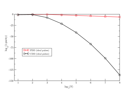
Figure 1: Simulation of PDD (square) and CDD (circles) for concatenation levels 1 to 8. Results shown are for one minus purity of the system qubit as a function of the number of pulses. The pulses used are ideal. Note the fantastically high purity achieved with CDD. In the case of PDD the horizontal axis gives $\log_{4}$ of the total number of pulses, while for CDD the numbers on the horizontal axis denote the concatenation level.

We performed a numerically exact simulation for comparing different pulse sequences for a qubit coupled to a small environment. We consider a spin chain of length $N$, where the central spin is from a different species (the electron in the dot versus the surrounding nuclei) and acts as the system qubit. The (undesired) couplings between the spins is given by Heisenberg interaction terms, so that the coupling Hamiltonians between two spins $i$ and $j$ at a distance $d$ (measured in units of the lattice constant) is given by $\frac{c}{2^{d}}(X_{i}X_{j}+Y_{i}Y_{j}+Z_{i}Z_{j})$, where $c$ depends on the species of the spins $i$ and $j$. We fix the coupling strengths and the number of spins so that the coupling strengths roughly correspond to GaAs our example: $J=1\text{MHz}$ and $\beta=10\text{KHz}$. The effective errors at the end of the concatenated cycles are so low (purity loss of around $10^{-100}$ – see Fig. 1) that we are forced to use extremely high precision linear algebra that significantly burdens simulation performance. To get practical results, we argue based on Lieb-Robinson bounds (see osborne:157202 ) that within the duration of the simulation, enlarging the spin chain will not modify the results. This was verified independently for a test case where there was no significant qualitative difference between $N=3,5,7$. Therefore the results presented here are for $N=3$ and they capture the essence of our estimates.

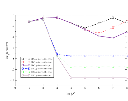
Figure 2: Simulation of PDD (squares) and CDD (circles) for concatenation levels 1 to 8 with non-ideal pulses. The pulse widths are set at 1ps, 10ps, and 100ps. Axes as in Fig. 1.

We fix the overall duration of the pulse sequence at $10^{-5}\text{s}$ so that $\beta T<1$ [see Eq. (28)]. This allows us to concentrate on the inter-pulse period and pulse-widths that are the main technological challenge for decoupling. Higher concatenation levels thus correspond to $\log(\text{number of pulses})$ [or to $\log(1/\text{inter-pulse period})$]. In Fig. 1, we compare CDD and PDD purities for ideal pulses at various levels of concatenation. The vertical axis displays the loss of purity of the system qubit, i.e., $1-\textrm{Tr}[(\rho_{S})^{2}]$, where $\rho_{S}=\textrm{Tr}_{B}(\rho)$, and $\rho$ is the joint system-bath density matrix at the final time $T$. The higher order data for PDD are obtained by simply repeating the basic sequence and shrinking the pulse-interval. This is necessary to get the long-term behavior of decoupling. The graphs show a progressive improvement in purity of the initial qubit state, $\frac{\left|0\right\rangle+\left|1\right\rangle}{\sqrt{2}}$, as a function of concatenation level. The environment part of the spin chain is initialized in a thermal state at a temperature of $1$K. In Fig. 2 we have depicted the effect of realistic pulse widths on decoupling. We note that in the case of PDD the performance of the pulse sequence deteriorates with increasing pulse width (as expected), but also (after an initial improvement, as in the ideal pulse case) as a function of the number of pulses used. This latter deterioration is somewhat surprising, and is due to the pulse width errors that simply accumulate over time. The point of deterioration shifts to the right as the pulse width is made smaller, as expected. The improvement seen for the $100$ps case at $\log_{4}(N)=7$ can be understood as being due to the essentially random-walk-on-a-circle-like nature of the accumulated errors, which will occassionally result in a recurrence. Concatenated sequences are naturally robust against these errors, as can be seen clearly in the figure, where CDD results in a saturation of the purity. The asymptotic purity level is roughly equal to the square of the per-pulse-error $\delta J$ (recall subsection III.3). For example, with $\delta=1$ps and $J=1$MHz we find $(\delta J)^{2}=10^{-12}$, in agreement with Fig. 2. While it is impossible to go to error rates below per-pulse-error, with concatenation we are able to maintain the error rate at this minimum.

V Higher Order (Trotter-Suzuki) Universal Decoupling

Suppose a universal dynamical decoupling sequence is known, i.e., essentially a series of unitarily transformed Hamiltonians $H_{j}=P_{j}H_{e}P_{j}^{{\dagger}}$ such that $\sum_{j}P_{j}H_{e}P_{j}^{{\dagger}}=B\otimes I_{S}$ for some environment operator $B$. As we saw previously, the sequential application of propagators generated by these Hamiltonians acts trivially on the system only up to the first order in $\|B_{\alpha}\|\tau_{0}$ where $\tau_{0}$ is a typical free-evolution period duration. Trotter-Suzuki expansion allows us to construct a sequence of these propagators that act trivially on the system up to any order $n$. Suppose $\{\epsilon A_{j}\}_{j=1}^{k}$ are dimensionless Hermitian operators such that $\sum A_{j}=A$ and $\epsilon$ is a small parameter. Trotter-Suzuki expansion allows us to find a sequence of indices $\{n_{i}\}_{i=1}^{N}$ ($n_{i}\in\{1\ldots k\}$) and real numbers $\{c_{i}\}_{i=1}^{N}$ such that

$$e^{\epsilon c_{1}A_{n_{1}}}e^{{\epsilon c_{2}A_{n_{2}}}}\ldots e^{{\epsilon c_{N}A_{n_{N}}}}=e^{\epsilon A+O(\epsilon^{n})}$$ (60)

The number $N$ of propagators required, scales with $e^{n^{2}}$. It is worth emphasizing that while numerous, the sequence of coefficients $c_{i}$ and indices $n_{i}$ can be constructed recursively Suzuki:76 ; Hatano:05 .

For practical purposes it is advantageous to use a variation on this expansion in which the coefficients $c_{i}$ are rational numbers. Once the sequence of propagators is known we can construct the Trotter-Suzuki decoupling sequence (TSDS) accordingly: Set up $A_{j}=iH_{j}$ and $A=iB\otimes I$ based on the universal DD cycle and employ the following DD sequence using the smallest pulse switching time $\tau_{\text{min}}$ available:

$$P_{n_{1}}\mathtt{f}[c_{1}\tau_{\text{min}}]P_{n_{1}}^{{\dagger}}P_{n_{2}}\mathtt{f}[c_{2}\tau_{\text{min}}]P_{n_{2}}^{{\dagger}}\ldots P_{n_{N}}\mathtt{f}[c_{N}\tau_{\text{min}}]P_{n_{N}}^{{\dagger}},$$ (61)

where $\mathtt{f}[\tau]$ denotes a free evolution period of duration $\tau$. By dimensional analysis, the error in Eq. (60), $\epsilon^{n}$, translates into left-over terms asymptotically bounded by products of operators $B_{\alpha}$ and is thus bounded by $O[(\tau_{\mathrm{min}}\max{\|B_{\alpha}\|})^{n}]$. We can thus asymptotically estimate the error phase as:

$$\Phi_{\text{TSDS}} = O\left[\left(\tau_{\text{min}}\max\{\|B_{\alpha}\|\}\right)^{n}\right]$$ (62)

$$= O\left[\left(T\max\{\|B_{\alpha}\|\}/N\right)^{\sqrt{\log N}}\right],$$

A serious problem is that negative $c_{i}$’s routinely appear in the TSDS (except for $n=3$). Clearly, this presents a major problem since one cannot have negative times in the free evolution segments in Eq. (61). For this reason, as presented the TSDS is not physically implementable. A solution for this problem is not yet available to us, but does not seem impossible.

Table (1) summarizes the asymptotic performance of PDD, CDD and TSDS in the limit of large number of pulses and the two regimes of $J<\beta$ and $\beta\ll J$.

DD Scheme	$\Phi$ for $J<\beta$	$\Phi$ for $\beta\ll J$
Periodic DD	$T^{2}\beta J/N$	$T^{2}J^{2}/N$
Concatenated DD	$(\beta T/N^{1/2})^{\log_{4}\!N}(JT)$	$N{({JT}/{N})}^{N^{\log_{4}(5/2)}}$
Trotter-Suzuki	$(\beta T/N)^{\sqrt{\log_{4}\!N}}$	$(JT/N)^{\sqrt{\log_{4}\!N}}$

Table 1: Asymptotic comparison of the error phase $\Phi$ for deterministic decoupling schemes. $T$ is the total experiment duration, $N$ the total number of pulses, $J$ and $\beta$ are defined in Eq. (18).

The TSDS performs remarkably well and is oblivious to the distinction between pure-bath and system-bath dynamics. Nonetheless, its performance is sensitive to small errors in pulse operation and the switching times that need to be precisely set (not required in PDD and CDD and randomized decoupling schemes). Thus it may not be a robust alternative to CDD, in spite of its superior convergence properties, but it may be used as a basic dynamical decoupling sequence at the base of a new concatenated pulse sequence. This is particularly useful with the TSDS at $n=3$.

Finally, we note that the Trotter-Suzuki expansion was also recently used by Brown et al. in a study of arbitrarily accurate composite pulse sequences Brown:04 . There the goal was to overcome systematic errors in the system control Hamiltonian, without considering decoherence.

VI Decoupling with Very Narrow Pulses Cannot Increase Error Norms

In this section we return to DD with ideal, zero width pulses, and argue that such DD sequences can never effectively strengthen the undesired terms and cannot cause extra errors. We then argue that even with finite-width, but sufficiently narrow pulses, error norms cannot increase under DD. These results are of independent interest and apply to any pulse-based error suppression strategy, including closed-loop quantum error correction.

Consider a sequence of ideal unitary operations $P_{i}$ applied to a quantum system (measurements can also be included by enlarging the Hilbert space), and suppose a sequence of intervals $\tau_{i}$ separates these operations, such that the pulse sequence is given by: $P_{1}{\small\mathtt{f}_{\tau_{1}}}P_{2}{\small\ldots\mathtt{f}_{\tau_{n-1}}}P_{n}$. In the absence of environmental couplings, the overall effect of the pulse sequence would be given by $Q_{n}=P_{1}\ldots P_{n}$ – the “ideal operation”. But in the presence of the environmental couplings in $H_{e}$, the overall propagator $U$ is modified by error terms. Letting $Q_{i}=P_{1}\ldots P_{i}$, we can define an effective unitary error operator corresponding to the whole sequence in the following manner:

$$U =P_{1}e^{-i\tau_{1}H_{e}}P_{2}e^{-i\tau_{2}H_{e}}P_{3}\ldots P_{n-1}e^{-i\tau_{n}H_{e}}P_{n}$$

$$=Q_{1}e^{-i\tau_{1}H_{e}}Q_{1}^{{\dagger}}Q_{2}e^{-i\tau_{2}H_{e}}Q_{2}^{{\dagger}}\ldots Q_{n-1}e^{-i\tau_{n-1}}Q_{n-1}^{{\dagger}}Q_{n}$$

$$=e^{-i\tau_{1}Q_{1}H_{e}Q_{1}^{{\dagger}}}e^{-i\tau_{2}Q_{2}H_{e}Q_{2}^{{\dagger}}}\ldots e^{-i\tau_{1}Q_{n-1}H_{e}Q_{n-1}^{{\dagger}}}Q_{n}$$

$$=:\exp(-iTH_{e}^{\prime})P_{1}\ldots P_{n}$$ (63)

Note that in the last line we have defined the overall duration $T=\sum\tau_{i}$, and isolated the effective error Hamiltonian $H_{e}^{\prime}$ from the desired, ideal unitary operation $Q_{n}=P_{1}\ldots P_{n}$.

As before, we use a unitary operator norm $\|.\|$ to compare the strength of the error Hamiltonians $H_{e}$ and $H_{e}^{\prime}$. Unitary operator norms Bhatia:book , such as the absolute difference between the largest and smallest eigenvalues, are invariant under unitary transformations (for unitary $U$, $\|UAU^{{\dagger}}\|=\|A\|$) and can be used as measures of fidelity errors in Hamiltonian error correction theory Terhal:04 . We now use the following existential theorem due to Thompson Thompson:86 ; Childs:03 : Let $A_{1}$, $A_{2}$ be Hermitian matrices. Then there exist unitaries $U_{1}$ and $U_{2}$ and a Hermitian matrix $A$ such that

$$e^{iA_{1}}e^{iA_{2}}=e^{iA};\hskip 14.22636ptA=U_{1}A_{1}U_{1}^{{\dagger}}+U_{2}A_{2}U_{2}^{{\dagger}}.$$

This theorem can be extended (induction on the number of exponentials) to products involving more than two matrix exponentials: $e^{iA_{1}}\cdots e^{iA_{n}}=e^{iA}$. Using Eq. (63) and Thompson’s theorem we have: $TH_{e}^{\prime}=\sum_{i}\tau_{i}U_{i}Q_{i}H_{e}Q_{i}^{{\dagger}}U_{i}^{{\dagger}}$, and we have the following inequality for the norm of $H_{e}^{\prime}$:

$$\|H_{e}^{\prime}\| =\frac{1}{T}\|\sum_{i}\tau_{i}U_{i}Q_{i}H_{e}Q_{i}^{{\dagger}}U_{i}^{{\dagger}}\|$$

$$\leq\frac{1}{T}\sum_{i}\tau_{i}\|U_{i}Q_{i}H_{e}Q_{i}^{{\dagger}}U_{i}^{{\dagger}}\|=\|H_{e}\|$$ (64)

Thus the norm of the effective error Hamiltonian does not increase under the action of ideal unitary operators.

In the case of non-ideal pulses carrying systematic errors per pulse (e.g., due to finite pulse-width), we can model the pulse error as a unitary error operator immediately preceding the ideal pulse. For single-qubit pulse errors due to finite pulse widths, one can again show that $\|H_{e}^{\prime}\|\leq\|H_{e}\|$ provided the pulse widths are small enough KhodjastehLidar:inprep . This allows us to use Thompson’s theorem to show that our argument in this section also applies to pulses of sufficiently narrow width on a single qubit. We expect this argument to apply to multi-qubit near-perfect operators in the presence of a bounded bath.

As a special case, this argument applies to dynamical decoupling. While positively reassuring that with ideal pulses the undesired couplings do not increase in strength, the present argument does not quantify the efficiency of dynamical decoupling. For this purpose we employed, above, approximations based on the Magnus expansion.

The same argument applies in a quantum error correction codes setting Knill:97a , in particular in non-Markovian fault-tolerance theory Aharonov:05 ; Aliferis:05 ; Terhal:04 , where a “time-resolved fault path” expansion has recently been used to decompose the action of errors in the course of a general evolution. Our argument can be used to further rationalize such expansions based on the fact that errors are well-behaved (in the sense of $\|H_{e}^{\prime}\|\leq\|H_{e}\|$) in the non-Markovian regime.

VII Summary and Discussion

Dynamical decoupling (DD) cannot be exactly analyzed without concrete reference to the details of the system-environment coupling, but an abstract picture of the interaction in terms of bounded environment operators – as pursued here – can yield useful performance estimates. Within this framework, we have provided an analytic estimate of the leading order decoupling error associated with the basic universal decoupling cycle for a qubit. We have analyzed and compared the performance of periodic DD (PDD) and concatenated DD (CDD) schemes. We have provided detailed calculations supporting the conclusion reported in KhodjastehLidar:04 , that CDD significantly outperforms PDD within practical boundaries of pulse parameter space. We have distinguished between two different limiting cases of fast versus slow environment dynamics. Fast dynamics of the environment limits the performance of higher order deterministic dynamical decoupling. This can be understood from the interaction picture, where the system-bath interaction Hamiltonian is fast fluctuating. Slow bath dynamics, on the other hand, can be exploited by CDD to result in super-exponential decoupling using an exponential number of pulses. Table 1 provides a convenient summary of the relative performance of PDD and CDD, as well as the new Trotter-Suzuki based pulse sequence we have introduced.

Our discussion was based on a pulsed control mode, but it is known that higher fidelities are possible via fine-tuned navigation of the control Hamiltonian Viola:02 . This direction can be especially useful when decoupling methods are to be used not for quantum state preservation but for performing an error-corrected quantum evolution. Dynamically error corrected evolution can also be achieved via a hybrid decoupling error correction method ByrdLidar:01a ; ByrdLidar:02a ; KhodjastehLidar:03 : Consider a stabilizer quantum error correcting code characterized by a stabilizer group of Pauli operators Calderbank:97 ; Gottesman:96 . Assume that this code corrects all single qubit errors, which means that each single qubit error anticommutes with at least one stabilizer generator. This anti-commutation condition translates into time reversal of the error, when exponentiated. Thus it is possible to use the generator set of the stabilizer to form a universal decoupling sequence for decoupling single qubit error terms on the code space. In this way decoupling integrates seamlessly with the encoded quantum operations on the code space generated by Hamiltonians written as the sum of normalizer elements of the code. This also allows us to perform quantum error detection and recovery within a hybrid decoupling-error correction setting, thus allowing the correction of errors in both the Markovian and the non-Markovian regimes KhodjastehLidar:inprep .

The open-loop approach of DD appears at first sight to be conceptually and practically very different from the method of closed-loop quantum error correcting codes Steane:99 . However, recent results on the theory of non-Markovian fault tolerant quantum error correction (FTQEC) Terhal:04 ; Aliferis:05 ; Aharonov:05 suggest that the error bounds applicable in the fault tolerant, concatenated version of DD are in fact very similar to the bounds relevant to FTQEC. Specifically, in both CDD and FTQEC it is essential that the system-bath interaction Hamiltonian is norm-bounded (see Refs. AlickiLidarZanardi:05 ; Alicki:07 for a critique of this assumption). In light of the much smaller degree of overhead involved in CDD, this suggests that in the non-Markovian regime one can profit significantly by incorporating CDD into a closed-loop QECC procedure. CDD can then remove the leading order bath-induced errors, while the QECC procedure can target primarily the random control errors for which CDD offers only limited protection.

We note that it is possible to view the CDD procedure as a discrete time dynamical system, whose ideal fixed point is a vanishing system-bath interaction. In this manner it should be possible to characterize the region of correctable errors using tools from the analysis of fixed points, and to incorporate perturbations of the pulse sequence. An analysis of CDD from this perspective may well be a fruitful endeavor. Indeed, there exists a dynamical maps approach to concatenated quantum error correction, which has proven to be very convenient in the analysis of the fault tolerance threshold Rahn:02 ; Fern:06 .

As a final comment we should emphasize that the ability to perform arbitrarily precise Hamiltonian control on the system Hamiltonian assumes a classical control mechanism, while every control system is really quantum in nature. Thus besides technological constraints, fundamental quantum fluctuations may limit the performance of DD as well, since perfect classical control simply does not exist. A systematic characterization of bounds on the fidelity of feedback-free error correction schemes such as DD, imposed by fundamental quantum fluctuations, is still an important open question.

Appendix A Validity of the Magnus Expansion

We analyze the convergence domain of approximations and the dynamical renormalization process, specifically as it applies to CDD. This recursive renormalization can be written as:

$$U^{(n+1)}:=\exp(-i\tau_{n+1}H_{e}^{(n+1)})=\prod\limits_{j=1}^{4}\exp(-i\tau_{n}H_{j}^{(n)})$$ (65)

where $\tau_{n+1}=4\tau_{n}$, i.e.,

$$\tau_{n}=4^{n}\tau_{0},$$ (66)

and where

$$H_{1}^{(n)} =B_{0}^{(n)}\otimes I+B_{X}^{(n)}\otimes X+B_{Y}^{(n)}\otimes Y+B_{Z}^{(n)}\otimes Z=IH_{e}^{(n)}I,$$

$$H_{2}^{(n)} =B_{0}^{(n)}\otimes I+B_{X}^{(n)}\otimes X-B_{Y}^{(n)}\otimes Y-B_{Z}^{(n)}\otimes Z=XH_{e}^{(n)}X,$$

$$H_{3}^{(n)} =B_{0}^{(n)}\otimes I-B_{X}^{(n)}\otimes X+B_{Y}^{(n)}\otimes Y-B_{Z}^{(n)}\otimes Z=YH_{e}^{(n)}Y,$$

$$H_{4}^{(n)} =B_{0}^{(n)}\otimes I-B_{X}^{(n)}\otimes X-B_{Y}^{(n)}\otimes Y+B_{Z}^{(n)}\otimes Z=ZH_{e}^{(n)}Z,$$ (67)

are the recursive generalization of Eqs. (8). The Magnus expansion of $U^{(n)}$ yields:

$$U^{(n)}=\exp(-i\tau_{n}H^{(n)})=\exp(\sum_{i=1}^{\infty}A_{i}^{(n)}),$$ (68)

whence

$$\tau_{n}H^{(n)}=i[A_{1}^{(n)}+A_{2}^{(n)}]+\tau_{n}C^{(n)},$$ (69)

where

$$A_{1}^{(n)} =-i\tau_{n-1}\sum_{i=1}^{4}H_{i}^{(n-1)},$$ (70)

$$A_{2}^{(n)} =-\frac{1}{2}\tau_{n-1}^{2}\sum_{1=i<j=4}[H_{j}^{(n-1)},H_{i}^{(n-1)}],$$ (71)

$$-i\tau_{n}C^{(n)} =\sum_{i=3}^{\infty}A_{i}^{(n)}=\sum_{i=3}^{\infty}m_{i}\tau_{n-1}^{i}\underset{i\text{ commutators}}{\underbrace{[H_{j}^{(n-1)},[H_{k}^{(n-1)},...]]}},$$ (72)

where $m_{i}$ is a numerical factor determined by explicit computation of the $i$th order Magnus expansion, and $C^{(n)}$ is an operator-valued correction to the second order Magnus expansion.

We would like to find an approximation for the $B_{\alpha}^{(n)}$. To do so we will first show that it is consistent to use the second order Magnus expansion for $H_{e}^{(n)}$, in the sense that

$$H_{1}^{(n)}=H_{e}^{(n)}\approx\frac{i}{\tau_{n}}(A_{1}^{(n)}+A_{2}^{(n)})=:\sum_{\alpha=0,X,Y,Z}\tilde{B}_{\alpha}^{(n)}\otimes S_{\alpha}\text{,}$$ (73)

where we can safely neglect $C^{(n)}$ [i.e., all $A_{i>2}^{(n)}$] as long as

$$\tau_{n}\beta\ll 1.$$ (74)

This is the recursive generalization of the result obtained above for $n=1$. Then the $\tilde{B}_{\alpha}^{(n)}$ will be the desired approximation to $B_{\alpha}^{(n)}$. The proof is by induction. We will require the following inequalities, satisfied for bounded operators $A$ and $B$ Bhatia:book :

$$\left\|[A,B]\right\| \leq 2\left\|A\right\|\left\|B\right\|,$$ (75)

$$\left\|AB\right\| \leq \left\|A\right\|\left\|B\right\|,$$ (76)

$$\left\|A+B\right\| \leq \left\|A\right\|+\left\|B\right\|.$$ (77)

Lemma 1

The following relations hold:

$$||C^{(n)}||\ll\frac{1}{\tau_{n}}||A_{2}^{(n)}||$$ (78)

and

$$||\tilde{B}_{\alpha}^{(n)}|| = O(\beta),\quad\alpha=X,Y,Z$$ (79)

$$B_{0}^{(n)} = B_{0}.$$ (80)

• We prove the lemma by induction. Let us call Eq. (78) “a($n$)”, Eq. (79) “b_α($n$)”, and Eq. (80) “b₀($n$)”. We have already established the case a($1$) [Eq. (19)], and b_α($1$) and b₀($1$) are based on our definitions and assumptions. We will show that (1) b_α($n-1$) & b₀($n-1$) $\Rightarrow$ a($n$), (2) b₀($n-1$) $\Rightarrow$ b₀($n$), and then (3) a($n$) & b_α($n-1$) $\Rightarrow$ b_α($n$). Recall all along that we have assumed $J<\beta$.

(1) Proof of a($n$): We have, using Eqs. (71),(72) and inequality (75)

$$\tau_{n}||C^{(n)}|| \leq\sum_{i=3}^{\infty}m_{i}\tau_{n-1}^{i}||\underset{i\text{ commutators}}{\underbrace{[H_{j}^{(n-1)},[H_{k}^{(n-1)},...]]}}||=O\left(\sum_{i=3}^{\infty}\tau_{n-1}^{i-2}\underset{i-2\text{ terms}}{\underbrace{(||H_{j}^{(n-1)}||\,||H_{k}^{(n-1)}||\cdots)}}||A_{2}^{(n)}||\right)$$

$$\overset{\text{b}_{\alpha}\text{(}n-1\text{) }\&\text{ b}_{0}\text{(}n-1\text{)}}{=}O\left(\sum_{i=3}^{\infty}\tau_{n-1}^{i-2}\beta^{i-2}||A_{2}^{(n)}||\right)\overset{\tau_{n-1}\beta\ll 1}{=}O(\tau_{n-1}\beta||A_{2}^{(n)}||)\ll||A_{2}^{(n)}||$$

(2) Proof of b₀($n$):

$$A_{1}^{(n)} =-i\tau_{n-1}\sum_{i=1}^{4}H_{i}^{(n-1)}=-i4\tau_{n-1}B_{0}^{(n-1)}\otimes I\overset{\text{b}_{0}\text{(}n-1\text{)}}{=}-i\tau_{n}B_{0}\otimes I.$$

(3) Proof of b_α($n$): From Eq. (73) we have

$$H_{e}^{(n)} =\sum_{\alpha=0,X,Y,Z}B_{\alpha}^{(n)}\otimes S_{\alpha}\overset{\text{a(}n\text{)}}{\approx}\frac{i}{\tau_{n}}(A_{1}^{(n)}+A_{2}^{(n)})=\sum_{\alpha=0,X,Y,Z}\tilde{B}_{\alpha}^{(n)}\otimes S_{\alpha}.$$

Since $A_{2}^{(n)}$ contains no pure-environment terms it determines the part contributing to the sum over $\alpha=X,Y,Z$:

$$\| \sum_{\alpha=X,Y,Z} \tilde{B}_{\alpha}^{(n)}\otimes S_{\alpha}\|=\frac{1}{\tau_{n}}||A_{2}^{(n)}||\overset{\text{Eq. (\ref{eq:A2n})}}{=}\frac{1}{\tau_{n}}||\frac{1}{2}\tau_{n-1}^{2}\sum_{1=i<j=4}[H_{j}^{(n-1)},H_{i}^{(n-1)}]||$$

$$\overset{\text{Ineq. (\ref{ineq:com})-(\ref{ineq:plu})}}{\leq} \frac{\tau_{n-1}^{2}}{4\tau_{n-1}}\sum_{1=i<j=4}||H_{j}^{(n-1)}||\,||H_{i}^{(n-1)}||\overset{\text{b}_{\alpha}\text{(}n-1\text{)}}{=}O(\tau_{n-1}J^{2})<O(\tau_{n-1}\beta^{2})<O(\beta).$$

Since the system operators all have $||S_{\alpha}||=O(1)$ and the environment operators $\tilde{B}_{\alpha}^{(n)}$ all have similar norm, we can conclude that, as required, $||\tilde{B}_{\alpha}^{(n)}||=O(\beta)$.

The upshot of this proof is the following:

Corollary 2

The recursive second-order Magnus expansion, Eq. (73), is a valid approximation provided we assume $\tau_{n}\beta\ll 1$.

The condition $\tau_{n}\beta\ll 1$ of course puts a physical upper limit on the number of levels of concatenation. Provided this condition is satisfied, it follows that, schematically, we have

$$H_{e},\tau_{0} \mapsto H_{e}^{(1)}\approx\frac{i}{\tau_{1}}(A_{1}^{(1)}+A_{2}^{(1)})=:\sum_{\alpha}\tilde{B}_{\alpha}^{(1)}\otimes S_{\alpha},$$

$$H_{e}^{(1)},4\tau_{0} \mapsto H_{e}^{(2)}\approx\frac{i}{\tau_{2}}(A_{1}^{(2)}+A_{2}^{(2)})=:\sum_{\alpha}\tilde{B}_{\alpha}^{(2)}\otimes S_{\alpha},$$

$$\vdots$$

$$H_{e}^{(n-1)},4^{n-1}\tau_{0} \mapsto H_{e}^{(n)}\approx\frac{i}{\tau_{n}}(A_{1}^{(n)}+A_{2}^{(n)})=:\sum_{\alpha}\tilde{B}_{\alpha}^{(n)}\otimes S_{\alpha}.$$ (81)

Note that in the body of the paper, for notational simplicity we dropped the tilde, with the convention being that we are only considering the environment operators defined by the second-order Magnus expansion.

Appendix B Finite Pulse Width Analysis for CDD

For brevity define

$$\beta_{\alpha}^{(n)}:=\|B_{\alpha}^{(n)}\|,\quad\beta_{\alpha}:=\beta_{\alpha}^{(0)},\quad\beta:=\beta_{0},$$ (82)

and use Ineqs. (75)-(77) to reproduce the recursive inequalities corresponding to $\beta_{\alpha}^{(n)}$ from Eqs. (29)-(32):

$$\beta_{0}^{(n)} =\beta,$$ (83)

$$\beta_{X}^{(n)} \leq 2(\tau_{n-1}-\delta)\beta\beta_{X}^{(n-1)}+\frac{\delta}{\tau_{n-1}}(\frac{1}{2}\beta_{X}+\frac{1}{\pi}\beta_{Y})$$ (84)

$$\beta_{Y}^{(n)} \leq(\tau_{n-1}-\delta)\beta\beta_{Y}^{(n-1)}+(\tau_{n-1}-2\delta)\beta_{X}^{(n-1)}\beta_{Z}^{(n-1)}$$

$$\hskip 14.22636pt+\frac{1}{\pi}\frac{\delta}{\tau_{n-1}}\beta_{Z}$$ (85)

$$\beta_{Z}^{(n)} \leq\delta\left[\frac{2}{\pi}\beta_{X}^{(n-1)}(\beta_{Z}+\beta_{X})+\beta_{Y}^{(n-1)}\beta_{X}\right]+\frac{\delta}{\tau_{n-1}}\beta_{Z}.$$ (86)

A necessary condition for convergence is $\beta_{\alpha}^{(1)}<\beta_{\alpha}^{(0)}\equiv\beta_{\alpha}$ for $\alpha=X,Y,Z$. Let us define constants $a,b$ such that

$$\beta_{Y}=a\beta_{X},\quad\beta_{Z}=b\beta_{X}.$$ (87)

Then we have for the $n=1$ case of Eq. (84)

$$\beta_{X}^{(1)}\leq 2(\tau_{0}-\delta)\beta\beta_{X}+\frac{\delta}{\tau_{0}}(\frac{1}{2}+\frac{a}{\pi})\beta_{X},$$ (88)

which must be smaller than $\beta_{X}$. We thus find the necessary condition

$$2(\tau_{0}-\delta)\beta+\frac{\delta}{\tau_{0}}(\frac{1}{2}+\frac{a}{\pi})<1.$$ (89)

Next consider the $n=1$ case of Eq. (86), and set it to be smaller than $\beta_{Z}$:

$$\beta_{Z}^{(1)}/\beta_{Z}\leq(\delta\beta_{X})\left[\frac{2}{\pi}(1+\frac{1}{b})+\frac{a}{b}\right]+\frac{\delta}{\tau_{0}}<1.$$ (90)

Both quantities $\delta\beta_{X},\delta/\tau_{0}$ are $\ll 1$ by our previous assumptions, so this inequality is automatically satisfied. Finally, consider the $n=1$ case of Eq. (85), and set it to be smaller than $\beta_{Y}$:

$$\beta_{Y}^{(1)}/\beta_{Y}\leq(\tau_{0}-\delta)\beta+(\tau_{0}-2\delta)\frac{b}{a}\beta_{X}+\frac{1}{\pi}\frac{\delta}{\tau_{0}}\frac{b}{a}<1.$$ (91)

We can simplify these results somewhat, as follows. We can replace $\beta_{X}$ by $J=\max(\left\|B_{X}\right\|,\left\|B_{Y}\right\|,\left\|B_{Z}\right\|)<\beta$ [Eq. (18)], and assume for simplicity $a=b=1$. We can then replace Ineqs. (89),(91) by

$$2(\tau_{0}-\delta)\beta+(\frac{1}{2}+\frac{1}{\pi})\frac{\delta}{\tau_{0}} < 1$$ (92)

$$(\tau_{0}-\delta)(\beta+J)-\delta J+\frac{1}{\pi}\frac{\delta}{\tau_{0}} < 1.$$ (93)

We can safely replace $J$ by $\beta$ (since $J<\beta$) and drop $\delta J$ . This turns the second inequality into $2(\tau_{0}-\delta)\beta+\frac{1}{\pi}\frac{\delta}{\tau_{0}}<1$, so it is subsumed by the first inequality.

Appendix C Concatenation of the CPMG pulse sequence

Consider an error Hamiltonian $H_{e}$ of the form

$$H_{e}=B_{z}\otimes Z+B_{0}\otimes I_{S}.$$

A simple dynamical decoupling sequence (also known as CPMG Carr:54 ; Meiboom:58 ) can decouple this error Hamiltonian:

$$\mathtt{p}_{1}=X\mathtt{f}X\mathtt{f}$$

where $\mathtt{f}$ denotes a free evolution interval of duration $\tau$. The propagator corresponding to this sequence is given by:

$$U=e^{-i\tau(-B_{z}\otimes Z+B_{0}\otimes I_{S})}e^{-i\tau(B_{z}\otimes Z+B_{0}\otimes I_{S})}.$$

A simple application of the Baker-Campbell-Hausdorf (BCH) Reinsch:00 expansion shows that $U$ can be written as

$$U=e^{-i2\tau(B_{0}\otimes I_{S}+F[B_{0},B_{Z}]\otimes Z)}$$

where $F[B_{0},B_{Z}]$ is a Hermitian operator in the Lie sub-algebra generated by $B_{0}$ and $B_{Z}$. One can show that $\|F[B_{0},B_{Z}]\|=O(\|B_{0}\|\|B_{Z}\|\tau)$ in the limit of $\tau\rightarrow 0$. We can thus use the same sequence for decoupling the undecoupled term $F[B_{0},B_{Z}]\otimes Z$ and construct 2nd and 3rd order CDD sequences:

$$\mathtt{p}_{2} =\mathtt{f}X\mathtt{f}\mathtt{f}X\mathtt{f}$$ (94)

$$\mathtt{p}_{3} =X\mathtt{f}X\mathtt{f}\mathtt{f}X\mathtt{f}X\mathtt{f}X\mathtt{f}\mathtt{f}X\mathtt{f}$$ (95)

Notice that concatenated CPMG requires far fewer pulses than concatenated universal DD. However, CPMG is not as robust with respect to systematic errors in the pulses as concatenated universal DD.

References

- (1) W.H. Zurek, Physics Today 44, 36 (1991).
- (2) R. Freeman, Spin Choreography: Basic Steps in High Resolution NMR (Oxford University Press, Oxford, 1998).
- (3) L. M. K. Vandersypen and I. L. Chuang, Rev. Mod. Phys. 76, 1037 (2004).
- (4) L. Viola, E. Knill and S. Lloyd, Phys. Rev. Lett. 82, 2417 (1999).
- (5) L. Viola and S. Lloyd, Phys. Rev. A 58, 2733 (1998).
- (6) P. Facchi, S. Tasaki, S. Pascazio, H. Nakazato, A. Tokuse, D.A. Lidar, Phys. Rev. A 71, 022302 (2005).
- (7) K. Shiokawa, D.A. Lidar, Phys. Rev. A 69, 030302(R) (2004).
- (8) M.S. Byrd and D.A. Lidar, Quant. Inf. Proc. 1, 19 (2001).
- (9) L. P. Pryadko and P. Sengupta, Phys. Rev. B 73, 085321 (2006).
- (10) P. Facchi, D.A. Lidar, and S. Pascazio, Phys. Rev. A 69, 032314 (2004).
- (11) L. Viola and E. Knill, Phys. Rev. Lett. 94, 060502 (2005).
- (12) L F. Santos and L. Viola, eprint quant-ph/0602168.
- (13) L. Viola and L.F. Santos, J. Mod. Optics, to be published (2007).
- (14) O. Kern and G. Alber, Phys. Rev. Lett. 95, 250501 (2005).
- (15) P. Zanardi, Phys. Lett. A 258, 77 (1999).
- (16) W. Magnus, Commun. Pure Appl. Math. 7, 649 (1954).
- (17) K. Khodjasteh and D.A. Lidar, Phys. Rev. Lett. 95, 180501 (2005).
- (18) M. Suzuki, Commun. Math. Phys. 51, 183 (1976).
- (19) D.A. Lidar, K.B. Whaley, in Irreversible Quantum Dynamics, Vol. 622 of Lecture Notes in Physics (Springer, Berlin, 2003), p. 83, eprint quant-ph/0301032.
- (20) This is not the only possibility; one may consider controlling the environment as well. See, e.g., A. Pechen and H. Rabitz, Phys. Rev. A 73, 062102 (2006).
- (21) L.-A. Wu, M.S. Byrd, D.A. Lidar, Phys. Rev. Lett. 89, 127901 (2002).
- (22) M.S. Byrd, D.A. Lidar, L.-A. Wu, and P. Zanardi, Phys. Rev. A 71, 052301 (2005).
- (23) P. Sengupta and L. P. Pryadko, Phys. Rev. Lett. 95, 037202 (2005).
- (24) P. C. Moan and J. A. Oteo, J. Math. Phys. 42, 501 (2001).
- (25) R. Bhatia, Matrix Analysis, No. 169 in Graduate Texts in Mathematics (Springer-Verlag, New York, 1997).
- (26) A. V. Khaetskii, D. Loss, L. Glazman, Phys. Rev. Lett. 88, 186802 (2002).
- (27) L. Viola and E. Knill, Phys. Rev. Lett. 90, 037901 (2003).
- (28) U. Haeberlen, High Resolution NMR in Solids, Advances in Magnetic Resonance Series, Supplement 1 (Academic Press, New York, 1976).
- (29) L.F. Santos and L. Viola, Phys. Rev. A 72, 062303 (2005).
- (30) W. Yao, R. Liu, and L. J. Sham, Phys. Rev. Lett. 98, 077602 (2007).
- (31) B.M. Terhal, G. Burkard, Phys. Rev. A 71, 012336 (2005).
- (32) I. A. Merkulov, Al. L. Efros, M. Rosen, Phys. Rev. B 65, 205309 (2002).
- (33) W.A. Coish, V.N. Golovach, J.C. Egues, and D. Loss, Physica Status Solidi (b) 243, 3658 (2006).
- (34) R. de Sousa, N. Shenvi, and K.B. Whaley, Phys. Rev. B 72, 045330 (2006).
- (35) H.Y. Carr and E.M. Purcell, Phys. Rev. 94, 630 (1954).
- (36) S. Meiboom and D. Gill, Rev. Sci. Instrum. 39, 6881 (1958).
- (37) T.J. Osborne, Phys. Rev. Lett. 97, 157202 (2006).
- (38) N. Hatano and M. Suzuki, eprint math-ph/0506007.
- (39) K.R. Brown, A.W. Harrow, I.L. Chuang, Phys. Rev. A 70, 052318 (2004).
- (40) R.C. Thompson, Linear Multilinear Algebra 19, 187 (1986).
- (41) A. M. Childs, H. L. Haselgrove, and M. A. Nielsen, Phys. Rev. A 68, 052311 (2003).
- (42) K. Khodjasteh, D.A. Lidar, in preparation.
- (43) E. Knill, R. Laflamme and W. Zurek, Proc. Roy. Soc. London Ser. A 454, 365 (1998).
- (44) D. Aharonov, A. Kitaev, J. Preskill, Phys. Rev. Lett. 96, 050504 (2006).
- (45) P. Aliferis, D. Gottesman, and J. Preskill, Quantum Inf. Comput. 6, 97 (2006).
- (46) M.S. Byrd and D.A. Lidar, Phys. Rev. Lett. 89, 047901 (2002).
- (47) M.S. Byrd and D.A. Lidar, J. Mod. Optics 50, 1285 (2003).
- (48) K. Khodjasteh and D.A. Lidar, Phys. Rev. A 68, 022322 (2003).
- (49) A.R. Calderbank, E.M. Rains, P.W. Shor, and N.J.A. Sloane, Phys. Rev. Lett. 78, 405 (1997).
- (50) D. Gottesman, Phys. Rev. A 54, 1862 (1996).
- (51) A.M. Steane, in Introduction to Quantum Computation and Information, edited by H.K. Lo, S. Popescu and T.P. Spiller (World Scientific, Singapore, 1999), pp. 184–212.
- (52) R. Alicki, D.A. Lidar, and P. Zanardi, Phys. Rev. A 73, 052311 (2006)
- (53) R. Alicki, eprint quant-ph/0702050.
- (54) B. Rahn, A.C. Doherty, and H. Mabuchi, Phys. Rev. A 66, 032304 (2002).
- (55) J. Fern, J. Kempe, S. Simic, S. Sastry, IEEE Trans. on Automatic Control 51, 448 (2006).
- (56) M.W. Reinsch, J. Math. Phys. 41, 2434 (2000).