Optimal Quantum Measurements of Expectation Values of Observables

Abstract

Experimental characterizations of a quantum system involve the measurement of expectation values of observables for a preparable state ${|}{\psi}{\rangle}$ of the quantum system. Such expectation values can be measured by repeatedly preparing ${|}{\psi}{\rangle}$ and coupling the system to an apparatus. For this method, the precision of the measured value scales as ${1\over\sqrt{N}}$ for $N$ repetitions of the experiment. For the problem of estimating the parameter $\phi$ in an evolution $e^{-i\phi H}$, it is possible to achieve precision $1\over N$ (the quantum metrology limit, see Giovannetti et al. (2006)) provided that sufficient information about $H$ and its spectrum is available. We consider the more general problem of estimating expectations of operators $A$ with minimal prior knowledge of $A$. We give explicit algorithms that approach precision $1\over N$ given a bound on the eigenvalues of $A$ or on their tail distribution. These algorithms are particularly useful for simulating quantum systems on quantum computers because they enable efficient measurement of observables and correlation functions. Our algorithms are based on a method for efficiently measuring the complex overlap of ${|}{\psi}{\rangle}$ and $U{|}{\psi}{\rangle}$, where $U$ is an implementable unitary operator. We explicitly consider the issue of confidence levels in measuring observables and overlaps and show that, as expected, confidence levels can be improved exponentially with linear overhead. We further show that the algorithms given here can typically be parallelized with minimal increase in resource usage.

I Introduction

Uncertainty relations such as Heisenberg’s set fundamental physical limits on the achievable precision when we extract information from a physical system. The goal of quantum metrology is to measure properties of states of quantum systems as precisely as possible given available resources. Typically, these properties are determined by experiments that involve repeated preparation of a quantum system in a state $\rho$ followed by a measurement. The property is derived from the measurement outcomes. Because the repetitions are statistically independent, the precision with which the property is obtained scales as ${1\over\sqrt{N}}$, where $N$ is the number of preparations performed. This is known as the standard quantum limit or the shot-noise limit, and it is associated with a purely classical statistical analysis of errors. It has been shown that in many cases of interest, the precision can be improved to ${1\over N}$ by using the same resources but with initial states entangled over multiple instances of the quantum system, or by preserving quantum coherence from one experiment to the next. It is known that it is usually not possible to attain a precision that scales better than ${1\over N}$. (See Giovannetti et al. (2004) for a review of quantum-enhanced measurements.) A setting where this limit can be achieved is the parameter estimation problem, where the property is given by the parameter $\phi$ in an evolution $e^{-i\phi H}$ for a known Hamiltonian $H$ Giovannetti et al. (2006), which captures some common measurement problems. The standard method for determining $\phi$ requires the ability to apply $e^{-i\phi H}$ and to prepare and measure an eigenstate of $H$ with known eigenvalue. If it is not possible to prepare such an eigenstate or if we wish to determine expectations with respect to arbitrary states, this method fails. Here we are interested in the more general and physically important expectation estimation problem, where the property to be determined is an expectation $\langle A\rangle=\mbox{tr}(A\rho)$ of an observable (Hermitian operator) or unitary $A$, for a possibly mixed state $\rho$. Both $A$ and $\rho$ are assumed to be experimentally sufficiently controllable, but other than a bound on the eigenvalues of $A$ or their tail distribution, no other properties of $A$ or $\rho$ need to be known. In particular, we need not be able to prepare eigenstates of $A$ or know the spectrum of $A$. The parameter estimation problem is a special instance of the expectation estimation problem. Parameter estimation reduces to the problem of determining $\mbox{tr}(e^{-i\phi H}{|}{\psi}{\rangle}{\langle}{\psi}{|})$ for ${|}{\psi}{\rangle}$ an eigenstate of $H$ with non-zero eigenvalue. We show that for solving the expectation estimation problem, precision scalings of ${1\over N^{1-\alpha}}$ for arbitrarily small $\alpha>0$ can be achieved with sequential algorithms, and the algorithms can be parallelized with minimal additional resources.

Our motivation for this work is the setting of quantum physics simulations on quantum computers. This is one of the most promising applications of quantum computing Feynman (1982) and enables a potentially exponential speedup for the correlation function evaluation problem Terhal and DiVincenzo (2000); Ortiz et al. (2001); Somma et al. (2003). The measurement of these correlation functions reduces to the measurement of the expectation of an operator for one or more states. Because the measurement takes place within a scalable quantum computer, the operators and states are manipulatable via arbitrarily low-error quantum gates. The quantum computational methods that have been described for the determination of these expectations have order ${1\over\sqrt{N}}$ precision. An example is the one-ancilla algorithm for measuring $\langle U\rangle=\mbox{tr}(U\rho)$ for unitary $U$ described in Ortiz et al. (2001); Somma et al. (2002); Miquel et al. (2002), which applies $U$ conditional on an ancilla ${\sf a}$ prepared in a superposition state (Fig. 1). Improving the precision without special knowledge of the operator or state requires more sophisticated algorithms.

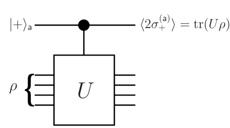
Figure 1: Quantum network for the one-ancilla algorithm to measure $\langle U\rangle=\mbox{tr}(U\rho)$ with ${|}{+}{\rangle}_{\sf a}=({|}{0}{\rangle}_{\sf a}+{|}{1}{\rangle}_{\sf a})/\sqrt{2}$ in the logical basis. The desired expectation is given by $\mbox{tr}(U\rho)=\langle 2\sigma_{+}^{\sf a}\rangle=\langle\sigma_{x}^{({\sf a})}\rangle+i\langle\sigma_{y}^{({\sf a})}\rangle$, where $\langle\sigma_{x}^{({\sf a})}\rangle$ and $\langle\sigma_{y}^{({\sf a})}\rangle$ are the expectations of the Pauli matrices $\sigma_{x}^{({\sf a})}$ and $\sigma_{y}^{({\sf a})}$ for the final state, which are estimated by repeating the experiment and measuring either $\sigma_{x}^{({\sf a})}$ or $\sigma_{y}^{({\sf a})}$ on the control (ancilla) qubit. Because these measurements have $\pm 1$ as possible outcomes, their statistics are determined by the binomial distribution.

Here we give quantum algorithms based on phase and amplitude estimation Cleve et al. (1998); Brassard et al. (2000) to improve the resource requirements to achieve a given precision. We begin by giving an “overlap estimation” algorithm (OEA) for determining the amplitude and phase of $\mbox{tr}(U\rho)$ for $U$ unitary. We assume that quantum procedures for preparing $\rho$ from a standard initial state and for applying $U$ are known and that it is possible to reverse these procedures. We determine the number of times $N$ that these procedures are used to achieve a goal precision $p$ and show that $N$ is of order $1/p$. To determine $\mbox{tr}(A\rho)$ for observables $A$ not expressible as a small sum of unitary operators, we assume that it is possible to evolve under $A$. This means that we can apply $e^{-iAt}$ for positive times $t$. The OEA can be used to obtain $\mbox{tr}(A\rho)t\approx i(\mbox{tr}(e^{-iAt}\rho)-1)$ for small $t$. The problem of how to measure $\mbox{tr}(A\rho)$ with precision $p$ requires determining $\mbox{tr}(e^{-iAt}\rho)$ with precision better than $pt$ and choosing $t$ small enough that the error in the approximation does not dominate. We solve this problem by means of an “expectation estimation” algorithm (EEA) with minimal additional knowledge on the eigenvalue distribution of $A$. For this situation, the relevant resources are not only the number $N$ of uses of $e^{-iAt}$ and of the state preparation algorithm, but also the total time $T$ of evolution under $A$. We show that to achieve a goal precision $p$, $N$ and $T$ are of order $1/(p^{1+\alpha})$ and $1/p$, respectively, with $\alpha>0$ arbitrarily small. The term $\alpha$ in the resource bound is due partly to the tail distribution of the eigenvalues of $A$ with respect to $\rho$. When it is known that $\rho$ is an eigenstate of $A$, so the distribution is a delta function, $\alpha=0$. This applies to the parameter estimation problem. In the case where $A$ is unbounded, $\alpha$ is still arbitrarily small if the tail distribution is exponentially decaying. But if only small moments of $A$ can be bounded, in which case the best bound on the tail distribution decays polynomially, $\alpha$ becomes finite.

It is important to properly define the meaning of the term “precision”. Here, when we say that we are measuring $\mbox{tr}(A\rho)$ with precision $p$, we mean that the probability that the measured value $a_{\mathrm{meas}}$ is within $p$ of $\mbox{tr}(A\rho)$ is bounded below by a constant $c>0$. In other words, the “confidence level” that $a_{\mathrm{meas}}-p\leq\mbox{tr}(A\rho)\leq a_{\mathrm{meas}}+p$ is at least $c$. Thus $a_{\mathrm{meas}}\pm p$ defines “confidence bounds” of the measurement for confidence level $c$. One interpretation of confidence levels is that if the measurement is independently repeated, the fraction of times the measured value is within the confidence bound is at least the confidence level. For measurement values $a_{\mathrm{meas}}$ that have an (approximately) gaussian distribution, it is conventional to use $c=0.68$ to identify the precision $p$ with the standard deviation. In this case, the confidence level that the measurement outcome is within $xp$ can be bounded by $\mathrm{erf}(x/\sqrt{2})$, where $\mathrm{erf}(y)$ is the error function, $\mathrm{erf}(x/\sqrt{2})\geq 1-e^{-x^{2}/2}$. This bound is often too optimistic, which is one reason to specify confidence levels explicitly. This becomes particularly important in our use of the “phase estimation” algorithm (PEA), whose standard version Cleve et al. (1998) has confidence levels that converge slowly toward $1$ with $x$. Because of these issues, our algorithms are stated so that they solve the problem of determining $\mbox{tr}(A\rho)$ with precision $p$ and confidence level $c$, where $p$ and $c$ are specified at the beginning. This requires that the resource usage be parameterized by both $p$ and $c$, and we show that the resource usage grows by a factor of order $|\log(1-c)|$ to achieve high confidence level $c$.

An important problem in measuring properties of quantum systems is how well the measurement can be parallelized with few additional resources. The goal of parallelizing is to minimize the time for the measurement by using more parallel resources. Ideally, the time for the measurement is independent of the problem. Typically we are satisfied if the time grows at most logarithmically. It is well known that for the parameter estimation problem, one can readily parallelize the measurement by exploiting entanglement in state preparation Bollinger et al. (1996). That this is still possible for the OEA and EEA given here is not obvious. In fact, we show that there are cases where parallelization either involves a loss of precision or requires additional resources. However, the entanglement method for parallelizing measurements works for expectation estimation and for overlap estimation when $|\mbox{tr}(U\rho)|$ is not close to $1$.

II Overlap Estimation

Let $U$ be a unitary operator and $\rho$ a state of quantum system $\mathsf{S}$. We assume that we can prepare $\rho$ and apply $U$ to any quantum system $\mathsf{S^{\prime}}$ that is equivalent to $\mathsf{S}$. Both the preparation procedure and $U$ must be reversible. In addition, we require that the quantum systems are sufficiently controllable and that $U$ can be applied conditionally (see below). We use labels to clarify which quantum system is involved. Thus, ${{\rho}^{({\mathsf{S^{\prime}}})}}$ is the state $\rho$ of system $\mathsf{S^{\prime}}$ and ${{U}^{({\mathsf{S^{\prime}}})}}$ is $U$ acting on system $\mathsf{S^{\prime}}$. This allows us to prepare $\rho$ and apply $U$ in parallel on multiple quantum systems.

When we say that we can prepare $\rho$, we mean that we can do this fully coherently. That is, we have access to a unitary operator $V^{(\mathsf{SE})}$ that can be applied to a standard initial state ${|}{0}{\rangle}_{{}_{\!\!\scriptstyle{\mathsf{SE}}}}$ of $\mathsf{S}$ and an ancillary system $\mathsf{E}$ (environment) such that ${{\rho}^{({\mathsf{S}})}}=\mbox{tr}_{\mathsf{E}}(V^{(\mathsf{SE})}{|}{0}{\rangle}_{{}_{\!\!\scriptstyle{\mathsf{SE}}}}\!\!{}^{\scriptstyle\mathsf{SE}}\!{\langle}{0}{|}(V^{(\mathsf{SE})})^{\dagger})$. The state $V^{(\mathsf{SE})}{|}{0}{\rangle}_{{}_{\!\!\scriptstyle{\mathsf{SE}}}}$ is a so-called purification of ${{\rho}^{({\mathsf{S}})}}$. For our purposes and without loss of generality, we can assume that $\rho$ is pure by merging systems $\mathsf{E}$ and $\mathsf{S}$ and letting unitaries act on the merged system. With this simplification we can write $\rho={|}{\psi}{\rangle}{\langle}{\psi}{|}=V{|}{0}{\rangle}{\langle}{0}{|}V^{\dagger}$ and use $\mathsf{S},\mathsf{S^{\prime}},\ldots$ to refer to equivalent merged systems. The goal of the OEA is now to estimate the overlap ${\langle}{\psi}{|}U{|}{\psi}{\rangle}$ of ${|}{\psi}{\rangle}$ with $U{|}{\psi}{\rangle}$.

The OEA and EEA require that $\mathsf{S}$ is sufficiently controllable. In particular, we require that it is possible to couple $\mathsf{S}$ to ancilla qubits and to implement conditional selective sign changes of ${|}{0}{\rangle}_{{}_{\!\!\scriptstyle{\mathsf{S}}}}$. Let ${{P_{0}}^{({\mathsf{S}})}}={{\mathbf{I}}^{({\mathsf{S}})}}-2{|}{0}{\rangle}_{{}_{\!\!\scriptstyle{\mathsf{S}}}}\!\!{}^{\scriptstyle\mathsf{S}}\!{\langle}{0}{|}$ be the selective sign change of ${|}{0}{\rangle}_{{}_{\!\!\scriptstyle{\mathsf{S}}}}$, with ${{\mathbf{I}}^{({\mathsf{S}})}}$ the identity (or no-action) operator. If an ancilla (control) qubit is labeled $\mathsf{a}$, an instance of the conditional selective sign change is defined by

$${{{{}^{c}\!P_{0}}}^{({\mathsf{aS}})}}={|}{0}{\rangle}_{{}_{\!\!\scriptstyle{\mathsf{a}}}}\!\!{}^{\scriptstyle\mathsf{a}}\!{\langle}{0}{|}{{\mathbf{I}}^{({\mathsf{S}})}}+{|}{1}{\rangle}_{{}_{\!\!\scriptstyle{\mathsf{a}}}}\!\!{}^{\scriptstyle\mathsf{a}}\!{\langle}{1}{|}{{P_{0}}^{({\mathsf{S}})}}.$$ (1)

If $\mathsf{S}$ consists of qubits and ${|}{0}{\rangle}_{{}_{\!\!\scriptstyle{\mathsf{S}}}}$ is the usual starting state with all qubits in logical state ${|}{0}{\rangle}$, then this is essentially a many-controlled sign flip and has efficient implementations Barenco et al. (1995).

As mentioned above, for the OEA we require that $U$ can be applied conditionally. This means that the unitary operator

$${{{{}^{c}\!U}}^{({\mathsf{aS}})}}={|}{0}{\rangle}_{{}_{\!\!\scriptstyle{\mathsf{a}}}}\!\!{}^{\scriptstyle\mathsf{a}}\!{\langle}{0}{|}{{\mathbf{I}}^{({\mathsf{S}})}}+{|}{1}{\rangle}_{{}_{\!\!\scriptstyle{\mathsf{a}}}}\!\!{}^{\scriptstyle\mathsf{a}}\!{\langle}{1}{|}{{U}^{({\mathsf{S}})}}$$ (2)

is available for use. When $U$ is associated with an evolution simulated on a quantum computer, this is no problem since all quantum gates are readily “conditionalized” Barenco et al. (1995). Nevertheless, we note that ${{}^{c}\!U}$ is not required if only the amplitude $|{\langle}{\psi}{|}U{|}{\psi}{\rangle}|$ of ${\langle}{\psi}{|}U{|}{\psi}{\rangle}$ is needed.

The “amplitude estimation” algorithm (AEA) Brassard et al. (2000) can almost immediately be applied to obtain $|{\langle}{\psi}{|}U{|}{\psi}{\rangle}|$. To accomplish our goals we need to adapt it for arbitrarily prepared states and use a version that avoids the complexities of the full quantum Fourier transform Shor (1997). Before we describe and analyze the version of the AEA needed here, we show how the OEA uses it to estimate the phase and amplitude of ${\langle}{\psi}{|}U{|}{\psi}{\rangle}$. Let $\mathrm{AE}(U,{|}{\psi}{\rangle},p)$ be the estimate of $|{\langle}{\psi}{|}U{|}{\psi}{\rangle}|$ obtained by the AEA for goal precision $p$. (We specify the meaning of the precision parameter below.)

• Given are $U$, ${|}{\psi}{\rangle}$ (in terms of a preparation unitary $V:{|}{0}{\rangle}\mapsto{|}{\psi}{\rangle}$) and the goal precision $p$. An estimate of ${\langle}{\psi}{|}U{|}{\psi}{\rangle}$ is to be returned.

• Obtain $a=\mathrm{AE}(U,{|}{\psi}{\rangle},p/4)$, so that $a$ is an estimate of $|{\langle}{\psi}{|}U{|}{\psi}{\rangle}|$ with precision $p/4$.

• Obtain $b_{0}=\mathrm{AE}({{{{}^{c}\!U}}^{({\mathsf{aS}})}},{|}{+\psi}{\rangle}_{{}_{\!\!\scriptstyle{\mathsf{aS}}}}={|}{+}{\rangle}_{{}_{\!\!\scriptstyle{\mathsf{a}}}}{|}{\psi}{\rangle},p/16)$.

  Note that ${}^{\scriptstyle\mathsf{aS}}\!{\langle}{+\psi}{|}{{{{}^{c}\!U}}^{({\mathsf{aS}})}}{|}{+\psi}{\rangle}_{{}_{\!\!\scriptstyle{\mathsf{aS}}}}=(1+{\langle}{\psi}{|}U{|}{\psi}{\rangle})/2$.

• Obtain $b_{\pi/2}=\mathrm{AE}(e^{i{{\sigma_{z}}^{({\mathsf{a}})}}\pi/4}{{{{}^{c}\!U}}^{({\mathsf{aS}})}},{|}{+\psi}{\rangle}_{{}_{\!\!\scriptstyle{\mathsf{aS}}}},p/16)$.

  Note that ${}^{\scriptstyle\mathsf{aS}}\!{\langle}{+\psi}{|}e^{i{{\sigma_{z}}^{({\mathsf{a}})}}\pi/4}{{{{}^{c}\!U}}^{({\mathsf{aS}})}}{|}{+\psi}{\rangle}_{{}_{\!\!\scriptstyle{\mathsf{aS}}}}=e^{i\pi/4}(1-i{\langle}{\psi}{|}U{|}{\psi}{\rangle})/2$.

• Estimate the phase $\theta$ of ${\langle}{\psi}{|}U{|}{\psi}{\rangle}$ by computing the argument of the complex number $y$ defined by

  $$\mathrm{Re}(y) = (4b_{0}^{2}-a^{2}-1)/2,$$

  $$\mathrm{Im}(y) = (4b_{\pi/2}^{2}-a^{2}-1)/2.$$ (3)

  If $a$, $b_{0}$ and $b_{\pi/2}$ were the exact values of the amplitudes estimated by the three instances of the AEA, then we would have $y={\langle}{\psi}{|}U{|}{\psi}{\rangle}$. For example, the formula for $\mathrm{Re}(y)$ may be obtained by geometrical reasoning, as shown in Fig. 2.

• Estimate ${\langle}{\psi}{|}U{|}{\psi}{\rangle}$ as $e^{i\theta}a$. The reason for not using $y$ directly is that if the overlap has amplitude near $1$, then the error in the amplitude of $y$ can be substantially larger than the error in $a$. (This is because of the way we estimate $y$ using a PEA; see below.)

We define $\mathrm{OE}(U,{|}{\psi}{\rangle},p)$ to be the value returned by the OEA. A flowchart for the algorithm is depicted in Fig. 3.

Figure 2: Geometrical construction for computing $\mathrm{Re}({\langle}{\psi}{|}U{|}{\psi}{\rangle})$ from $a=|{\langle}{\psi}{|}U{|}{\psi}{\rangle}|$ and $2b_{0}=|(1+{\langle}{\psi}{|}U{|}{\psi}{\rangle})|$. According to the law of cosines, $(2b_{0})^{2}=a^{2}+1+2a\cos(\theta)$, and we have $\mathrm{Re}({\langle}{\psi}{|}U{|}{\psi}{\rangle})=a\cos(\theta)=((2b_{0})^{2}-a^{2}-1)/2$.

Figure 3: OEA flowchart. An estimate of the overlap $\langle\psi|U|\psi\rangle$ is obtained. The algorithm requires three state preparations and calls the AEA three times. The amplitude of the returned value shown in the flowchart may need to be adjusted according to the value of $a$ to optimize the precision. For details see the text.

When $a=|{\langle}{\psi}{|}U{|}{\psi}{\rangle}|$ is close to $1$, the absolute precision with which $a$ is obtained is as much as quadratically better for the same resources. To avoid this nonuniformity of the precision to resource relationship, we define the precision $\delta$ of an overlap by means of a parameterization of ${\langle}{\psi}{|}U{|}{\psi}{\rangle}$ using the points $(x_{1},x_{2},x_{3})$ on the upper hemisphere of the surface of a unit sphere in three dimensions. For this purpose, define $h(x_{1},x_{2},x_{3})=x_{1}+ix_{2}$ for $x_{1}^{2}+x_{2}^{2}+x_{3}^{2}=1$ and $x_{3}\geq 0$. Define the distance between $(x_{1},x_{2},x_{3})$ and $(x_{1}^{\prime},x_{2}^{\prime},x_{3}^{\prime})$ to be the angular distance along a great circle. The precision of the value $o$ returned by the OEA is determined by the distance $\delta$ between the liftings $h^{-1}(o)$ and $h^{-1}({\langle}{\psi}{|}U{|}{\psi}{\rangle})$ (see Fig. 4). We define the precision of the value returned by the AEA similarly, by restricting the parametrization to the positive reals. The precision parameters with which the AEA is called in the OEA are chosen so that the returned overlap has precision $\delta\leq p$ with respect to our parametrization (see Note not (a)).

Figure 4: Visualization of the parameterization of the overlap in terms of points on the upper hemisphere of a unit sphere. The function $h$ is defined by $h(x_{1},x_{2},x_{3})=x_{1}+ix_{2}$. Note that for overlaps $|{\langle}{\psi}{|}U{|}{\psi}{\rangle}|$ approaching $1$ and small $\delta$, $\delta^{\prime}$ approaches $\delta^{2}/2\ll\delta$.

The AEA is based on a trick for converting amplitude into phase information, so that an efficient PEA can be applied. Let ${|}{\psi_{0}}{\rangle}={|}{\psi}{\rangle}$ and ${|}{\psi_{1}}{\rangle}=U{|}{\psi}{\rangle}$. Let $S_{0}=\mathbf{I}-2{|}{\psi_{0}}{\rangle}{\langle}{\psi_{0}}{|}=VP_{0}V^{\dagger}$ be the selective sign change of ${|}{\psi_{0}}{\rangle}$ and $S_{1}=\mathbf{I}-2{|}{\psi_{1}}{\rangle}{\langle}{\psi_{1}}{|}=UVP_{0}V^{\dagger}U^{\dagger}$ the selective sign change of ${|}{\psi_{1}}{\rangle}$. The composition $S=S_{0}S_{1}$ is a unitary operator that rotates ${|}{\psi_{0}}{\rangle}$ toward ${|}{\psi_{1}}{\rangle}$ in the two-dimensional subspace ${\cal Q}$ spanned by ${|}{\psi_{0}}{\rangle}$ and ${|}{\psi_{1}}{\rangle}$. The rotation is by a Bloch-sphere angle of $2\phi=4\arccos(|\langle\psi_{0}|\psi_{1}\rangle|)$. Thus, the eigenvalues of $S$ in ${\cal Q}$ are $e^{\pm i\phi}$. The Bloch sphere picture of the states and the rotation are shown in Fig. 5. When $|\langle\psi_{0}|\psi_{1}\rangle|=|{\langle}{\psi}{|}U{|}{\psi}{\rangle}|=1$, $S$ is the identity operator. The PEA for $S$ with initial state ${|}{\psi_{0}}{\rangle}$ determines the phase $\phi$ of one of these eigenvalues, where each of the signs has equal probability of being returned. The overlap $|{\langle}{\psi}{|}U{|}{\psi}{\rangle}|$ is obtained from $\phi$ by the formula $|{\langle}{\psi}{|}U{|}{\psi}{\rangle}|=\cos(\phi/2)$. The PEA requires use of the conditional $S$ operator, ${{}^{c}\!S}$. As defined, this needs to be decomposed into a product of ${{}^{c}\!P_{0}}$, ${{}^{c}\!U}$ and ${{}^{c}\!V}$. A significant simplification is to not condition $U$ and $V$ and to write ${{}^{c}\!S}=V{{}^{c}\!P_{0}}V^{\dagger}UV{{}^{c}\!P_{0}}V^{\dagger}U^{\dagger}$. This works because if the controlling qubit is in state ${|}{0}{\rangle}$, all the $U$’s and $V$’s are canceled by matching $U^{\dagger}$’s and $V^{\dagger}$’s Somma et al. (2002).

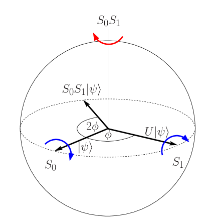
Figure 5: Bloch sphere picture of the rotations induced on the subspace spanned by ${|}{\psi}{\rangle}$ and $U{|}{\psi}{\rangle}$ by the operators $S_{0}$ and $S_{1}$.

Let $\mathrm{PE}(W,{|}{\psi^{\prime}}{\rangle},p)$ be a phase returned by the PEA for unitary operator $W$ and initial state ${|}{\psi^{\prime}}{\rangle}$ with precision goal $p$. The AEA may be summarized as follows.

• Given are $U$, ${|}{\psi}{\rangle}$ (in terms of a preparation unitary $V:{|}{0}{\rangle}\mapsto{|}{\psi}{\rangle}$) and the goal precision $p$. An estimate of $|{\langle}{\psi}{|}U{|}{\psi}{\rangle}|$ is to be returned.

• Let $\phi=\mathrm{PE}(S,{|}{\psi}{\rangle},2p)$ with $S=S_{0}S_{1}=VP_{0}V^{\dagger}UVP_{0}V^{\dagger}U^{\dagger}$.

• Estimate $|{\langle}{\psi}{|}U{|}{\psi}{\rangle}|$ as $|\cos(\phi/2)|$.

The precision parameter for the PEA has the conventional interpretation (modulo $2\pi$). Because $\arccos(|{\langle}{\psi}{|}U{|}{\psi}{\rangle}|)$ is the angle along the semicircle in the parametrization of the overlap defined above, the precision $2p$ of the value returned by the PEA translates directly to the desired precision in the value to be returned by the AEA.

The PEA Cleve et al. (1998) for a unitary operator $W$ and initial state ${|}{\psi^{\prime}}{\rangle}$ returns an estimate of the phase $\phi$ (“eigenphase”) of an eigenvalue $e^{i\phi}$ of $W$, where the probability of $\phi$ is given by the probability amplitude of ${|}{\psi^{\prime}}{\rangle}$ in the $e^{i\phi}$-eigenspace of $W$. In the limit of perfect precision, it acts as a von Neumann measurement of $W$ on state ${|}{\psi^{\prime}}{\rangle}$ in the sense that the final state is projected onto the $e^{i\phi}$-eigenspace of $W$. For finite precision, the eigenspaces may be decohered and the projection is incomplete, unless there are no other eigenvalues within the precision bound. The error in the projection is related to the confidence level with which the precision bound holds.

The original PEA is based on the binary quantum Fourier transform Shor (1997). It determines an eigenphase $\phi$ with precision $1\over 2^{n}$ with $2^{n}-1$ uses of the conditional ${{}^{c}\!W}$ operator to obtain a phase kickback to ancilla qubits. The original PEA begins by preparing $n$ qubits labeled $\mathsf{1}\ldots\mathsf{n}$ in state ${|}{+}{\rangle}_{{}_{\!\!\scriptstyle{\mathsf{1}}}}\ldots{|}{+}{\rangle}_{{}_{\!\!\scriptstyle{\mathsf{n}}}}$ and system $\mathsf{S}$ in state ${|}{\psi^{\prime}}{\rangle}_{{}_{\!\!\scriptstyle{\mathsf{S}}}}$. Next, for each $m=1,\ldots,n$, ${{}^{c}\!W}$ is applied from qubit $\mathsf{m}$ to system $\mathsf{S}$ $2^{m-1}$ times. The binary quantum Fourier transform is applied to the $n$ qubits, and the qubits are measured in the logical basis ${|}{0}{\rangle},{|}{1}{\rangle}$. The measurement outcomes give the first $n$ digits of the binary representation of $\phi/(2\pi)+\epsilon/2^{n}$, where $|\epsilon|<1/2$ with probability at least $0.405$ Cleve et al. (1998).

The PEA as outlined in the previous paragraph makes suboptimal use of quantum resources. We prefer a one-qubit version of the algorithm based on the measured quantum Fourier transform Griffiths and Niu (1996) that has been experimentally implemented on an ion trap quantum computer Chiaverini et al. (2005). An advantage of this approach is that it does not require understanding the quantum Fourier transform and is readily related to more conventional approaches for measuring phases. To understand how the algorithm given below works, note that the eigenstates of $W$ are invariant under ${{}^{c}\!W}$. The only interaction with $\mathsf{S}$ is via uses of ${{}^{c}\!W}$. Therefore, without loss of generality, we can assume that $\mathsf{S}$ is initially projected to an $e^{i\phi}$-eigenstate of $W$ with $0\leq\phi<2\pi$. The bits of an approximation of $\phi/(2\pi)$ are determined one by one, starting with the least significant one that we wish to learn. Given $n$, let $[.b_{1}\ldots b_{n}]_{2}=\sum_{i=1}^{n}b_{i}/2^{i}$ (with $b_{i}=0,1$) be a best $n$-digit binary approximation to $\phi/(2\pi)$, where the notation $[x]_{2}$ is used to convert a sequence of binary digits $x$ to the number that it represents. Write $\epsilon=(\phi/(2\pi)-[.b_{1}\ldots b_{n}]_{2})2^{n}$.

• Given are $W$, ${|}{\psi^{\prime}}{\rangle}$ (as a state of a quantum system) and the goal precision $p$. An estimate of an eigenphase $\phi$ of $W$ is to be returned, where the probability of $\phi$ is given by the population of ${|}{\psi^{\prime}}{\rangle}$ in the corresponding eigenspace.

• Let $n$ be the smallest natural number such that $2^{n}\geq 1/p$.

  • Prepare ${|}{+}{\rangle}_{{}_{\!\!\scriptstyle{\mathsf{a}}}}$ in an ancilla qubit $\mathsf{a}$ and apply ${{{{}^{c}\!W}}^{({\mathsf{aS}})}}$ $2^{n-1}$ times. With the auxiliary assumption that ${|}{\psi^{\prime}}{\rangle}$ is an $e^{i\phi}$-eigenstate of $W$, the effect is a phase kickback, changing ${|}{+}{\rangle}_{{}_{\!\!\scriptstyle{\mathsf{a}}}}$ to $({|}{0}{\rangle}_{{}_{\!\!\scriptstyle{\mathsf{a}}}}+e^{i2^{n-1}\phi}{|}{1}{\rangle}_{{}_{\!\!\scriptstyle{\mathsf{a}}}})/\sqrt{2}$.

  • Measure $\mathsf{a}$ in the ${|}{+}{\rangle},{|}{-}{\rangle}$ basis, so that measurement outcome $0$ ($1$) is associated with detecting ${|}{+}{\rangle}$ (${|}{-}{\rangle}$). Let $b^{\prime}_{n}$ be the measurement outcome. With the auxiliary assumption, the probability that $b^{\prime}_{n}=b_{n}$ is $\cos(\pi\epsilon/2)^{2}$.

• Do the following for each $k=(n-1),\ldots,1$:

  • Prepare ${|}{+}{\rangle}_{{}_{\!\!\scriptstyle{\mathsf{a}}}}$ in an ancilla qubit $\mathsf{a}$ and apply ${{{{}^{c}\!W}}^{({\mathsf{aS}})}}$ $2^{k-1}$ times. With the auxiliary assumption, this changes ${|}{+}{\rangle}_{{}_{\!\!\scriptstyle{\mathsf{a}}}}$ to $({|}{0}{\rangle}_{{}_{\!\!\scriptstyle{\mathsf{a}}}}+e^{i2^{k-1}\phi}{|}{1}{\rangle}_{{}_{\!\!\scriptstyle{\mathsf{a}}}})/\sqrt{2}$.

  • Compensate the phase of ${|}{1}{\rangle}_{{}_{\!\!\scriptstyle{\mathsf{a}}}}$ by changing it by $e^{-i\pi[.b^{\prime}_{k+1}\ldots b^{\prime}_{n}]_{2}}$. With the auxiliary assumption, this changes the state of the ancilla to $({|}{0}{\rangle}_{{}_{\!\!\scriptstyle{\mathsf{a}}}}+e^{i(2^{k-1}\phi-\pi[.b^{\prime}_{k+1}\ldots b^{\prime}_{n}]_{2})}{|}{1}{\rangle}_{{}_{\!\!\scriptstyle{\mathsf{a}}}})/\sqrt{2}$.

  • Measure $\mathsf{a}$ in the ${|}{+}{\rangle},{|}{-}{\rangle}$ basis to obtain $b^{\prime}_{k}$. With the auxiliary assumption and if $b^{\prime}_{l}=b_{l}$ for $l>k$, the probability that $b^{\prime}_{k}=b_{k}$ is $\cos(\pi\epsilon/2^{n-k+1})^{2}$.

• Estimate $\phi$ as $2\pi[.b^{\prime}_{1}\ldots b^{\prime}_{n}]_{2}$.

A step of the algorithm is depicted in Fig. 6.

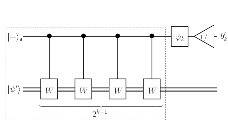
Figure 6: Step 2 of the PEA to estimate bit $k$ of the eigenphase, where $k=3$. The phase $\hat{\varphi}_{k}$ is computed according to previously obtained information about the eigenphase. By applying it before the measurement, the probability of obtaining the optimal value for bit $k$ is maximized. The measurement is denoted by the triangle pointing left with $+/-$ inside and is a measurement in the ${|}{+}{\rangle}/{|}{-}{\rangle}$ basis. The outlined part of the network will be parallelized in Sect. V.

The probability $P(\epsilon)$ that the value returned by the PEA is $2\pi[.b_{1}\ldots b_{n}]_{2}$ is the product of the probabilities $\cos(\pi\epsilon/2^{l})^{2}$ for $l=1,\ldots,n$ and is bounded below by $\sin(\pi\epsilon)^{2}/(\pi\epsilon)^{2}$. This bound can be obtained by taking the limit $n\rightarrow\infty$ in $P(\epsilon)$. The worst case is given for $|\epsilon|=1/2$, leading to the bound $P(\epsilon)\geq 4/\pi^{2}\approx 0.405$ Cleve et al. (1998). Since the goal precision is $2^{-n}$, it is acceptable for the algorithm to obtain the next best binary approximation to $\phi$. For this, the value obtained for $b_{n}^{\prime}$ may not be the one with maximum probability, but the subsequent bits $b_{k}^{\prime}$ are always the best possible given $b_{n}^{\prime}$. Taking this into account, the probability that the phase returned is within $2^{-n}$ is given by $P(\epsilon)+P(1-\epsilon)\geq 8/\pi^{2}\approx 0.81$ (see Note not (b)).

The key step of the one-qubit phase estimation procedure is to modify the phase kickback by the previously obtained phase estimate. This differentiates it from an adaptive phase measurement method that determines the bits of an approximation of $\phi/(2\pi)$ starting with the most significant bit, and making sufficiently many measurements with different phase compensations for each bit to achieve high confidence level. This is the phase estimation method given in Kitaev (1995) and mentioned in Giovannetti et al. (2006), which approximates what is done in practice for the efficient determination of an unknown frequency or pulse time.

The resources required by the PEA, AEA and OEA can be summarized as follows.

• This requires $N(p)=2^{\lceil\log_{2}(1/p)\rceil}-1$ uses of $W$. ${|}{\psi^{\prime}}{\rangle}$ is prepared once. Here, $\lceil x\rceil$ denotes the least integer $m\geq x$.

• This calls $\mathrm{PE}$ once. It requires $N(2p)$ uses of $S=VP_{0}V^{\dagger}UVP_{0}V^{\dagger}U^{\dagger}$ and one use of $V$ to prepare the initial state. We count this as being equivalent to $4N(2p)+1$ state preparations and $2N(2p)$ applications of $U$.

• This contains three calls to the AEA with higher precision. The total resource count is $8N(p/8)+4N(p/2)+3$ state preparations and $4N(p/8)+2N(p/2)$ uses of $U$.

Since $N(p)$ is of order $1/p$, each of these algorithms uses resources of order $1/p$.

III Confidence Bounds

The PEA as described in the previous section obtains an estimate $\phi_{\mathrm{est}}$ of an eigenphase $\phi$ such that the prior probability that $\left|\phi_{\mathrm{est}}-\phi\right|<2^{-n+1}\pi$ is at least $0.81$, regardless of the value of $\phi$, where $n=\lceil\log_{2}(1/p)\rceil$. (The comparison of $\phi_{\mathrm{est}}$ to $\phi$ is modulo $2\pi$, so that $\left|\phi_{\mathrm{est}}-\phi\right|$ is angular distance between $e^{i\phi_{\mathrm{est}}}$ and $e^{i\phi}$.) Thus, after having obtained $\phi_{\mathrm{est}}$, we say that $\phi=\phi_{\mathrm{est}}\pm 2^{-n+1}\pi$ with confidence level $0.81$ or $P[\phi_{\mathrm{est}}-2^{-n+1}\pi<\phi<\phi_{\mathrm{est}}+2^{-n+1}\pi]=0.81$. The error bound of $2^{-n+1}\pi$ must not be confused with a standard deviation. Suppose that we use a single sample from a gaussian distribution with standard deviation $\sigma$ to infer the mean. We would expect that the confidence level increases as $1-e^{-\Omega((\Delta/\sigma)^{2})}$ for an error bound of $\Delta$. (The notation $\Omega(x)$ means a quantity asymptotically bounded below by something proportional to $x$, that is, there exists a constant $C>0$ such that the quantity is eventually bounded below by $Cx$.) In general, it is desirable to have confidence levels that increase at least exponentially as a function of distance $\Delta$ or as a function of additional resources used. Unfortunately, for a single instance of the PEA, we cannot do better than have confidence level $1-O(1/\Delta)$ for $\phi=\phi_{\mathrm{est}}\pm 2^{-n+1}\pi\Delta$ Cleve et al. (1998). (Here, $O(x)$ denotes a quantity that is of order $x$, that is a quantity that is eventually bounded above by $Cx$ for some constant $C$. The meaning of “eventually” depends on context. Here it means “for sufficiently small $x$”. If the asymptotics of the argument require that it go to infinity, it means “for sufficiently large $x$”.) The method suggested in Cleve et al. (1998) for increasing the confidence level is to use the PEA with a higher goal precision of $p/2^{l}$. However this improves the confidence level on $\phi=\phi_{\mathrm{est}}\pm 2^{-n+1}\pi\Delta$ to only $1-\Omega(1/(\Delta 2^{l}))$ and requires a $2^{l}$ resource overhead, which is not an efficient improvement in confidence level.

A reasonable goal is to attain confidence level $c=1-e^{-\Omega(r)}$ that $\phi=\phi_{\mathrm{est}}\pm 2^{-n+1}\pi$ with a resource overhead of a factor of $O(r)$. This modifies the resource counts from the previous section from $O(1/p)$ to $O(|\log(1-c)|/p)$, where $c$ is the confidence level achieved. To attain this goal, we modify each step of the PEA by including repetition to improve the confidence level that acceptable values for the bits are determined. Let the two nearest $n$-digit binary approximations to $\phi/(2\pi)$ be given by $\phi/(2\pi)=[.b_{1}\ldots b_{n}]_{2}+\delta/2^{n}$ and $\phi/(2\pi)=[.\tilde{b}_{1}\ldots\tilde{b}_{n}]_{2}+(\delta-1)/2^{n}$, where $0\leq\delta<1$. We wish to obtain one of these approximations with high confidence level. For the first step of the PEA, we perform two sets of $r$ experiments to obtain a good estimate of $\delta^{\prime}=\pi(\delta+b_{n})$. The first set consists of $r$ $({|}{+}{\rangle}_{{}_{\!\!\scriptstyle{\mathsf{a}}}},{|}{-}{\rangle}_{{}_{\!\!\scriptstyle{\mathsf{a}}}})$-measurements of the state ${{}^{c}\!W}^{2^{n-1}}{|}{+}{\rangle}_{{}_{\!\!\scriptstyle{\mathsf{a}}}}{|}{\psi}{\rangle}_{{}_{\!\!\scriptstyle{\mathsf{S}}}}$. The second consists of $r$ $({|}{+}{\rangle}_{{}_{\!\!\scriptstyle{\mathsf{a}}}},{|}{-}{\rangle}_{{}_{\!\!\scriptstyle{\mathsf{a}}}})$-measurements of the state ${{}^{c}\!W}^{2^{n-1}}({|}{0}{\rangle}_{{}_{\!\!\scriptstyle{\mathsf{a}}}}-i{|}{1}{\rangle}_{{}_{\!\!\scriptstyle{\mathsf{a}}}})/\sqrt{2}{|}{\psi}{\rangle}_{{}_{\!\!\scriptstyle{\mathsf{S}}}}$. Let $x_{1},x_{2}$ be the sample means of the measurement outcomes of the two sets of experiments. In the limit of large $r$, $x_{1}$ and $x_{2}$ approach $\sin(\delta^{\prime}/2)^{2}$ and $\sin(\delta^{\prime}/2-\pi/4)^{2}$, respectively. We have

$$\sin(\delta^{\prime})=\cos(\delta^{\prime}-\pi/2)=1-2\sin(\delta^{\prime}/2-\pi/4)^{2},\;\cos(\delta^{\prime})=1-2\sin(\delta^{\prime}/2)^{2},$$ (4)

so we can estimate $\delta^{\prime}$ from $x_{1}$ and $x_{2}$ by letting $\delta^{\prime}_{\mathrm{est}}$ be the phase of the complex vector $(1-2x_{1})+i(1-2x_{2})$. The probability of the event $E$ that $\delta^{\prime}$ differs from $\delta^{\prime}_{\mathrm{est}}$ by more than $\pi/4$ modulo $2\pi$ can be bounded as follows. For this event, $|\sin(\delta^{\prime})+i\cos(\delta^{\prime})-((1-2x_{1})+i(1-2x_{2}))|^{2}\geq 1/2$. It follows that either $|\sin(\delta^{\prime}/2)^{2}-x_{1}|\geq 1/4$ or $|\sin(\delta^{\prime}/2-\pi/4)^{2}-x_{2}|\geq 1/4$. The probability of each of these possibilities is bounded by the probability that the mean of $r$ samples of the binomial distribution with probability $p$ of outcome $1$ differs from $p$ by at least $x=1/4$. The probability of this event is bounded by $2e^{-2rx^{2}}=2e^{-r/8}$ (Hoeffding’s bound Hoeffding (1963)). This bound can now be doubled to obtain a bound of $4e^{-r/8}$ on the probability of $E$.

Let $a_{n}=1$ if $\delta^{\prime}_{\mathrm{est}}$ is closer to $\pi$ than $0$, and $a_{n}=0$ otherwise. Then $a_{n}=b_{n}$ or $a_{n}=\tilde{b}_{n}$. Which equality holds does not affect the subsequent arguments, so without loss of generality, assume that $a_{n}=b_{n}$. Suppose that event $E$ did not happen and that we have correctly obtained $a_{n}=b_{n},\ldots,a_{k+1}=b_{k+1}$. For the step of the algorithm that determines the $k$’th bit, modify the original step by compensating the phase of ${|}{1}{\rangle}_{{}_{\!\!\scriptstyle{\mathsf{a}}}}$ by $e^{-i(\pi[.b_{k+1}\ldots b_{n-1}]_{2}+\delta^{\prime}_{\mathrm{est}}/2^{n-k})}$ and repeating the measurement $r$ times. We set $a_{k}=1$ if the majority of the measurement outcomes is $1$ and $a_{k}=0$ otherwise. For each measurement, the probability that the measurement outcome does not agree with $b_{k}$ is at most $\sin((\delta^{\prime}-\delta^{\prime}_{\mathrm{est}})/2^{n-k+1})^{2}$. Our assumptions imply that this is at most $\sin(\pi/2^{n-k+3})^{2}\leq(\pi/2^{n-k+3})^{2}$. Using Hoeffding’s bound again, the probability that $a_{k}\not=b_{k}$ is bounded by $2e^{-2r(1/2-(\pi/2^{n-k+3})^{2})}<2e^{-r/2}$ (for a loose upper bound).

Summing the probabilities, we find that the probability that we do not learn $b_{1}\ldots b_{n}$ or $\tilde{b}_{1}\ldots\tilde{b}_{n}$ is bounded by $x(n,r)=2(n-1)e^{-r/2}+4e^{-r/8}$. We can therefore say that the modified PEA yields the desired phase to within $\pi/2^{n-1}$ with confidence level $1-x(n,r)$, where $x(n,r)$ decreases exponentially in $r$. Note again that this confidence bound still should not be confused with a similar confidence bound for a gaussian random variable. Increasing the confidence bound does not result in the expected increase in confidence level. In order to have confidence level increasing exponentially toward $1$ with increasing confidence bound and an additional overhead of at most $O(|\log(p)|)$, we can repeat the determination of the $k$’th bit $2^{n-k}r$ instead of $r$ many times.

For the purpose of having high confidence level in the precision with which a quantity is estimated, our algorithms require the confidence level goal as an input. The modified PEA may be outlined as follows.

• Given are $W$, ${|}{\psi^{\prime}}{\rangle}_{{}_{\!\!\scriptstyle{\mathsf{S}}}}$, a goal precision $p$ and a goal confidence level $c$. An eigenphase $\phi$ of $W$ is to be returned, where the probability of $\phi$ is given by the population of ${|}{\psi^{\prime}}{\rangle}$ in the corresponding eigenspace. The final state of $\mathsf{S}$ consists of states with eigenphases in the range $\phi\pm p$ with prior probability at least $c$.

• Let $n$ be the smallest natural number such that $2^{n}\geq 1/p$. Let $r$ be the smallest natural number such that $x(n,r)<(1-c)$.

• Obtain $\delta^{\prime}_{\mathrm{est}}$ with the two sets of $r$ measurements described above. Let $a_{n}=1$ if $\delta^{\prime}_{\mathrm{est}}$ is closer to $\pi$ than $0$ and $a_{n}=0$ otherwise.

• Do the following for each $k=(n-1),\ldots,1$, in this order:

  • Obtain an estimate of the $k$’th bit $a_{k}$ of a binary approximation to $\phi/(2\pi)$ by $r$ repetitions of the measurement of steps 2.a-c given previously, but with a phase compensation that uses $\delta^{\prime}_{\mathrm{est}}$ as well as the previously obtained bits.

• Return $2\pi[.a_{1}\ldots a_{n}]_{2}$.

We define $\mathrm{PE}(W,{|}{\psi^{\prime}}{\rangle},p,c)$ to be the value returned by the modified PEA.

The resources required grow by a factor of less than $2r$, where $r=O(|\log(1-c)|)$. The constant hidden by the order notation may be determined from the expression for $r$ in step 0 and is not very large. To modify the AEA to attain confidence level $c$, it suffices to change the call to $\mathrm{PE}$ by including $c$ as an argument. Because the OEA has three independent calls to the AEA, it needs to make these calls with confidence level arguments of $1-(1-c)/3$ to ensure that the final confidence level is $c$. The resource requirements of all three algorithms are $O(|\log(1-c)|/p)$, where this applies to both the uses of $U$ and of the state preparation operator $V$ in the case of the AEA and OEA.

IV Expectation Estimation

Let $A$ be an observable and assume that it is possible to evolve under $\pm A$ for any amount of time. This means that we can implement the unitary operator $e^{-iAt}$ for any $t$. The traditional idealized procedure for measuring $\langle A\rangle=\mbox{tr}(A\rho)$ is to adjoin a system consisting of a quantum particle in one dimension with momentum observable $\hat{p}$ and apply the coupled evolution $e^{-iA\otimes\hat{p}}$ to the initial state $\rho\otimes{|}{0}{\rangle}{\langle}{0}{|}$, where ${|}{0}{\rangle}$ is the position “eigenstate” with eigenvalue $0$. Measuring the position of the particle yields a sample from the distribution of eigenvalues of $A$ von Neumann (1971); Ortiz et al. (2001). This procedure requires unbounded energy, both for preparing ${|}{0}{\rangle}$ and to implement the coupled evolution. Performing this measurement $N$ times yields an estimate of $\langle A\rangle$ with precision of order $\mathrm{var}(A)/\sqrt{N}$, where the variance is $\mathrm{var}(A)=\langle(A-\langle A\rangle)^{2}\rangle$. It is desirable to improve the precision and to properly account for the resources required to implement the coupling.

We focus on measurement methods that can be implemented in a quantum information processor. In order to accomplish this, some prior knowledge of the distribution of eigenvalues of $A$ with respect to $\rho$ is required. Suppose we have an upper bound $b$ on $|\mbox{tr}(A\rho)|$ and a bound on the tail distribution $F(\Delta)\geq\mbox{tr}([|A-\langle A\rangle|>\Delta]\rho)$, where $[|A-\langle A\rangle|>\Delta]$ denotes the projection operator onto eigenspaces of $A$ with eigenvalues $\lambda$ satisfying $|\lambda-\langle A\rangle|>\Delta$. That is, $F(\Delta)\geq\sum_{|\lambda-\langle A\rangle|>\Delta}p_{\lambda}$ with $p_{\lambda}=\mbox{tr}({|}{\lambda}{\rangle}{\langle}{\lambda}{|}\rho)$. Without loss of generality, $F$ is non-increasing in $\Delta$. An estimate on the tail distribution is needed to guarantee the confidence bounds on $\mbox{tr}(A\rho)$ derived from measurements by finite means. Here are some examples: If the maximum eigenvalue of $A$ is $\lambda_{\mathrm{max}}$, we can set $b=\lambda_{\mathrm{max}}$ and use $F(\Delta)=1$ if $\Delta<\lambda_{\mathrm{max}}$ and $F(\Delta)=0$, otherwise. Suppose that we have an upper bound $v$ on the variance $\mathrm{var}(A)$. If we know that the distribution of eigenvalues of $A$ is gaussian, we can estimate $F(\Delta)$ by means of the error function for gaussian distributions. With no such prior knowledge, the best estimate is $F(\Delta)=\min(1,v/\Delta^{2})$. (Observe that $v\geq\Delta^{2}\sum_{|\lambda-\langle A\rangle|>\Delta}p_{\lambda}$.) Such “polynomial” tails result in significant overheads for measuring $\langle A\rangle$. “Good” tails should drop off at least exponentially for large $\Delta$ (“exponential tails”).

We give an EEA based on overlap estimation. The relevant resources for the EEA are the number $M$ of times a unitary operator of the form $e^{-iAt}$ is used, the total time $T$ that we evolve under $A$, and the number $N$ of preparations of $\rho$. The total time $T$ is the sum of the absolute values of exponents $t$ in uses of $e^{-iAt}$. For applying the OEA, it is necessary to be able to evolve under $-\!A$ as well as $A$. If the evolution is implemented by means of quantum networks, this poses no difficulty. However, if the evolution uses physical Hamiltonians, this is a nontrivial requirement. The complexity of realizing $e^{-iAt}$ may depend on $t$ and the precision required. Since this is strongly dependent on $A$ and the methods used for evolving under $A$, we do not take this into consideration and assume that the error in the implementation of $e^{-iAt}$ is sufficiently small compared to the goal precision. In most cases of interest this is justified by results such as those in Berry et al. (2005), which show that for a large class of operators $A$, $e^{-iAt}$ can be implemented with resources of order $t^{1+\alpha^{\prime}}/\epsilon^{\alpha^{\prime}}$, where $\epsilon$ is the error of the implementation and $\alpha^{\prime}$ is arbitrarily small.

For exponential tails $F$, our algorithm achieves $M,N=O(1/p^{1+\alpha})$ and $T=O(1/p)$ for arbitrarily small $\alpha$. The order notation hides constants and an initialization cost that depends on $b$ and $F$. The strategy of the algorithm is to measure $\mbox{tr}(e^{-iAt}\rho)$ for various $t$. In the limit of small $t$, $\mbox{tr}(e^{-iAt}\rho)=1+O(t^{2})-i(\langle A\rangle t+O(t^{3}))$, so that $\langle A\rangle$ can be determined to $O(t^{3})$ from the imaginary part of $\mbox{tr}(e^{-iAt}\rho)$. The first problem is to make an initial determination of $\langle A\rangle$ to within a deviation of $A$ as determined by $F$. This is an issue when $b$ is large compared to the deviation. To solve the first problem, we can use phase estimation. We also give a more efficient method based on amplitude estimation. The second problem is to avoid excessive resources to achieve the desired precision while making $t$ small. To solve this problem requires choosing $t$ carefully and taking advantage of higher-order approximations of $\langle A\rangle$ by linear combinations of $\mbox{tr}(e^{-iAt}\rho)$ for different times $t$.

To bound the systematic error in the approximation of $\langle A\rangle$ by $i\mbox{tr}(e^{-iAt}\rho)$, note that $|\mathrm{Im}(e^{i\theta})-\theta|\leq\theta^{3}/6$. To see this it is sufficient to bound the Lagrange remainder of the Taylor series of $\sin(\theta)$. This bound suffices for achieving $\alpha=1/2$ in the bounds on $M$ and $N$. Reducing $\alpha$ requires a better approximation, which we can derive from the Taylor series of the principal branch of $\ln(x+1)$. For $|x|<1$,

$$|\ln(x+1)-\sum_{k=1}^{K}(-1)^{k-1}x^{k}/k|\leq|x|^{K+1}/((K+1)(1-|x|)^{K+1}).$$ (5)

To apply these series to the problem of approximating $\langle A\rangle$, we compute

$$\sum_{k=1}^{K}(-1)^{k-1}(e^{-iBt}-1)^{k}/k=\sum_{l=0}^{K}C_{l}e^{-iBlt},$$ (6)

for real constants $C_{l}$ satisfying $|C_{l}|\leq 2^{K}$. In particular, if $B$ is an operator satisfying $|B|<x/t$, we can estimate

$$\left|t\,\mbox{tr}(B\rho)+\sum_{l=0}^{K}C_{l}\ \mathrm{Im}\ \mbox{tr}(e^{-iBlt}\rho)\right|\leq|x|^{K+1}/((K+1)(1-|x|)^{K+1}).$$ (7)

Define $G_{e}(\Delta)=\Delta F(\Delta)+\int_{\Delta}^{\infty}F(s)ds$. Then $G_{e}(\Delta)$ is an upper bound on the contribution to the mean from eigenvalues of $A$ that differ from the mean by more than $\Delta$. That is, $G_{e}(\Delta)\geq\mbox{tr}(|A-\langle A\rangle|[|A-\langle A\rangle|>\Delta]\rho)=\sum_{|\lambda-\langle A\rangle|>\Delta}|\lambda-\langle A\rangle|\ p_{\lambda}$. Like $F(\Delta)$, $G_{e}(\Delta)$ is non-increasing. We assume that a non-increasing bound $G(\Delta)\geq G_{e}(\Delta)$ is known and that $G(\Delta)\rightarrow 0$ as $\Delta\rightarrow\infty$. Because $F(\Delta)\leq G_{e}(\Delta)/\Delta$, we can use $G$ to bound both $G_{e}$ and $F$. For $x>0$, define $G^{-1}(x)=\inf\{\Delta|G(\Delta)\leq x\}$. The behavior of $G^{-1}$ as $x$ goes to $0$ determines the resource requirements for the EEA. If $A$ is a bounded operator with bound $\lambda_{\mathrm{\max}}$, then we can use $G^{-1}(x)\leq\lambda_{\mathrm{max}}$ independent of $x>0$. If $F$ is exponentially decaying, then so is $G$, and $G^{-1}(x)=O(|\log(x)|)$. For polynomial tails with $F(\Delta)=O(1/\Delta^{2+\beta})$, we have $G(\Delta)=O(1/\Delta^{1+\beta})$ and $G^{-1}(x)=O(1/x^{1/(1+\beta)})$.

The EEA has two stages. The first is an initialization procedure to determine $\langle A\rangle$ with an initial precision that is of the order of a bound on the deviation of $A$ from its mean, where the deviation is determined from $F$ and $G$. This initialization procedure involves phase estimation to sample from the eigenvalue distribution of $A$. Its purpose is to remove offsets in the case where the expectation of $A$ may be very large compared to the width of the distribution of eigenvalues as bounded by $F$ and $G$. The second stage zooms in on $\mbox{tr}(A\rho)$ by use of the overlap estimation procedure. As before, we can assume without loss of generality that $\rho$ is pure, $\rho={|}{\psi}{\rangle}{\langle}{\psi}{|}$. We first give a version of the EEA that achieves $M,N=O(1/p^{3/2})$ and then refine the algorithm to achieve better asymptotic efficiency.

• Given are $A$, ${|}{\psi}{\rangle}$ (in terms of a preparation unitary $V:{|}{0}{\rangle}\mapsto{|}{\psi}{\rangle}$), a goal precision $p$ and the desired confidence level $c$. The returned value is within $p$ of $\langle A\rangle=\mbox{tr}(A{|}{\psi}{\rangle}{\langle}{\psi}{|})$ with probability at least $c$.

  • Choose $\Delta$ such that $F(\Delta/2)<1/4$ and $\Delta\geq p$. $\Delta$ should be chosen as small as possible. Let $t_{i}=\pi/(4(b+\Delta))$. Let $r$ be the minimum natural number such that $2e^{-r/8}\leq(1-c)/4$ and set $c^{\prime}$ according to the identity $r(1-c^{\prime})=(1-c)/4$.

  • Obtain $\Lambda_{1},\ldots,\Lambda_{r}$ from $r$ instances of the PEA, $\Lambda_{k}=\mathrm{PE}(e^{-iAt_{i}},{|}{\psi}{\rangle},\Delta t_{i}/2,c^{\prime})$, where $2\pi$ is subtracted for any return values between $\pi$ and $2\pi$ to ensure that $-\pi\leq\Lambda_{k}<\pi$.

  • Let $\Lambda_{m}$ be the median of $\Lambda_{1},\ldots,\Lambda_{r}$. We show below that the probability that $|\Lambda_{m}/t_{i}+\langle A\rangle|>\Delta$ is bounded by $2e^{-r/8}+r(1-c^{\prime})\leq(1-c)/2$.

  • Let $a_{0}=-\Lambda_{m}/t_{i}$. We expect $a_{0}$ to be within $\Delta$ of $\langle A\rangle$ with confidence level $1-(1-c)/2$.

  • If $p=\Delta$, return $a_{0}$ and skip this stage.

  • Choose $\theta_{\max}$ and $t$ so that they satisfy

    $$\begin{array}[b]{lrcl}\textrm{(A)}&\theta_{\max}^{3}/6&\leq&(t/2)p/4,\\ \textrm{(B)}&G(\theta_{\max}/t)&\leq&\theta_{\max}p/8,\\ \textrm{(C)}&\theta_{\max}&\leq&1,\\ \textrm{(D)}&t\Delta&\leq&\theta_{\max}.\end{array}$$ (8)

    The constraints and how they can be satisfied are explained below. The parameter $t$ should be chosen as large as possible to minimize resource requirements.

  • Obtain $x={\rm OE}(e^{-i(A-a_{0})(t/2)},{|}{\psi}{\rangle},(t/2)p/4,1-(1-c)/2)$.

  • Return $-\mathrm{Im}(x)/(t/2)+a_{0}$.

Consider stage I of the algorithm. The probability that $|\Lambda_{m}/t_{i}+\langle A\rangle|>\Delta$ may be bounded as follows. The choice of $t_{i}$ ensures that eigenvalues $\Lambda$ of $-At_{i}$ within $\Delta t_{i}$ of the mean are between $\pm\pi/4$ and do not get “aliased” by $e^{-iAt_{i}}$ in the calls to the PEA. With probability at least $1-r(1-c^{\prime})$, each $\Lambda_{k}$ returned by these calls is within $t_{i}\Delta/2$ of an eigenvalue of $-At_{i}$ sampled according to the probability distribution induced by ${|}{\psi}{\rangle}$. Assume that the event described in the previous sentence occurred. The probability that $|\Lambda_{m}/t_{i}+\langle A\rangle|>\Delta$ is upper bounded by the probability that at least $\lceil r/2\rceil$ of the $r$ samples fall outside the range $[-\langle A\rangle t_{i}-\Delta t_{i},-\langle A\rangle t_{i}+\Delta t_{i}]$. The choice of $\Delta$ with respect to $F$ implies that Hoeffding’s bound can be applied to bound this probability by $2e^{-r/8}$. Thus, we can bound the overall prior probability $P$ that $|\Lambda_{m}/t_{i}+\langle A\rangle|>\Delta$ by $P<2e^{-r/8}+r(1-c^{\prime})\leq(1-c)/2$.

The resources required for stage I include $N=r=O(|\log(1-c)|)$ preparations of ${|}{\psi}{\rangle}$, $M=O(|\log(1-c)|(b+\Delta)/\Delta)$ uses of $e^{-iAs}$ (specifically, $M$ is within a factor of $2$ of $2r/\Delta t_{i}$) and a total evolution time of $T=O(|\log(1-c)|/\Delta)$ (where $T$ is within a factor of $2$ of $2r\Delta$). Note that none of these resource bounds depend on the $p$ and that $\Delta$ is a bound on a deviation of $A$ from the mean with respect to ${|}{\psi}{\rangle}$. Also, if $\Delta$ is of the same order as $b$, the formulation of stage I of the algorithm is such that the uses of phase estimation require minimal precision. In fact, in this case, stage I of the algorithm could be skipped with minor adjustments to stage II. We show below that stage I can be modified so that the overhead as a function of $b$ is logarithmic. The modification requires that the number of state preparations $N$ is of the same order as $M$.

In the special case of parameter estimation (see the introduction), $\Delta=p$. Consequently stage II is skipped and the resources of stage I are the total resources required. The algorithm therefore achieves the optimal $O(1/p)$ resource requirements for this situation.

Consider stage II of the algorithm. The error $|-\mathrm{Im}(x)/(t/2)+a_{0}-\langle A\rangle|$ may be bounded as follows. We assume that all the precision constraints of stage I and II are satisfied. The confidence level that this is true is $c$ overall. With this assumption, $x/(t/2)$ is within $p/4$ (the “precision error”) of $\mbox{tr}(e^{-i(A-a_{0})(t/2)}\rho)/(t/2)$. There are three contributions to the “approximation error”, which is the difference between $-\mathrm{Im}\,\mbox{tr}(e^{-i(A-a_{0})(t/2)}\rho)/(t/2)$ and $\mbox{tr}((A-a_{0})\rho)$. For all contributions, we have to consider the fact that $a_{0}$ approximates $\langle A\rangle$ to within only $\Delta$, which is why we need constraint (D) of Eq. (8). The first arises from eigenvalues of $(A-a_{0})(t/2)$ in $[-\theta_{\max},+\theta_{\max}]$ due to $|\mathrm{Im}(e^{i\theta})-\theta|$ not being zero and is bounded by $\theta_{\max}^{3}/(6(t/2))=p/4$ (constraint (A) of Eq. (8)). The second and third come from eigenvalues of $(A-a_{0})(t/2)$ outside $[-\theta_{\max},+\theta_{\max}]$. Constraint (D) of Eq. (8) implies that $|(a_{0}-\langle A\rangle)(t/2)|\leq\theta_{\max}/2$. Constraints (B) and (C) of Eq. (8) imply that the contribution to $\langle A\rangle$ of eigenvalues differing from the mean by more than $\theta_{\max}/(2(t/2))$ is at most $\theta_{\max}p/8\leq p/8$. However the same eigenvalues still contribute to the measurement, each contributing at most $1$ to $x$. Constraint (B) of Eq. (8) together with the inequality $F(\Delta)\leq G(\Delta)/\Delta$ imply that $F(\theta_{\max}/(2(t/2)))\leq tp/8$ so this contribution has probability at most $tp/8$ and therefore adds at most another $p/4$ (after dividing by $t/2$) to the approximation error. Thus, the combination of the approximation and precision error is less than $p$, as desired. Clearly these estimates are suboptimal, tighter choices of $\theta_{\max}$ and $t$ could be made. However, this does not affect the asymptotics of the resource requirements.

To find good solutions $\theta_{\max}$ and $t$ subject to the constraints given in Eq. (8), we can rewrite the constraints as follows:

$$\begin{array}[t]{lc}\textrm{(A')}&G^{-1}(\theta_{\max}p/8)\leq\theta_{\max}/t\leq(p/8)/(\theta_{\max}^{2}/6),\\ \textrm{(B')}&\theta_{\max}\leq 1,\;\theta_{\max}/t\geq\Delta.\end{array}$$ (9)

The first inequality of (A’) is implied by constraint (B) and the second by constraint (A) of Eq. (8). To satisfy these constraints, we first find $\theta_{\max}\leq 1$ as large as possible so that

$$\begin{array}[c]{lc}\textrm{(A'')}&\Delta\leq G^{-1}(\theta_{\rm max}p/8)\leq(p/8)/(\theta_{\max}^{2}/6),\end{array}$$ (10)

and then set $t=\theta_{\max}/G^{-1}(\theta_{\max}p/8)$. Consider the three examples of bounded, exponential and polynomial tails. For the case of bounded tails, constraint (A”) of Eq. (10) can be solved by setting $\theta_{\max}$ according to $\lambda_{\max}=(p/8)/(\theta_{\max}^{2}/6)$, so that $\theta_{\max}=(3p/(4\lambda_{\max}))^{1/2}$. The parameter $t$ is given by $\theta_{\max}/\lambda_{\max}=(3p/4)^{1/2}/\lambda_{\max}^{3/2}=\Omega(p^{1/2})$. For the case of exponential tails, we can use $G^{-1}(x)=O(|\log(x)|)$ to show that $\theta_{\max}=\Omega((p/|\log(p)|)^{1/2})$ and $t=\Omega(p^{1/2}/|\log(p)|^{3/2})$ (see Note not (c)). For polynomial tails with $G^{-1}(x)=O(x^{-1/(1+\beta)})$, we get $\theta_{\max}=\Omega(p^{(2+\beta)/(1+2\beta)})$ and $t=\Omega(p^{(5+6\beta+\beta^{2})/((1+\beta)(1+2\beta))})$ (see Note not (d)).

The resource requirements for stage II of the EEA can be estimated as $M=O(|\log(1-c)|/tp)$ uses of an exponential of the form $e^{-iAs}$, $N=O(|\log(1-c)|/tp)$ state preparations, and a total time of $T=O(|\log(1-c)|/p)$, in terms of the parameter $t$ computed in step 0 (of stage II). The dependence on $G$ shows up in the value of $t$. With $t$ as computed in the previous paragraph, for bounded $A$, $M$ and $N$ are $O(|\log(1-c)|/p^{3/2})$. For exponential tails, $M$ and $N$ are $O(|\log(1-c)|/(p/|\log(p)|)^{3/2})$. For polynomial tails, they are $O(|\log(1-c)|/p^{\gamma(\beta)})$, where $\gamma(\beta)$ is a polynomial satisfying $\gamma(\beta)\rightarrow 1+1/2$ for $\beta\rightarrow\infty$ and $\gamma(\beta)=1+5$ for $\beta=0$.

To reduce the resource requirements of stage II of the EEA, we use overlap estimation at multiple values of $t$ and Eq. (6). Here is the modified stage. We assume that $K\geq 2$.

• Choose $\theta_{\max}$ and $t$ so that they satisfy

  $$\begin{array}[b]{lrcl}\textrm{(A)}&\theta_{\max}^{K+1}/((K+1)(1-\theta_{\max})^{K+1})&\leq&(t/2)p/4,\\ \textrm{(B)}&G(\theta_{\max}/t)&\leq&\theta_{\max}p/(8K2^{K}),\\ \textrm{(C)}&\theta_{\max}&\leq&1,\\ \textrm{(D)}&t\Delta&\leq&\theta_{\max}.\end{array}$$ (11)

  The parameter $t$ should be chosen as large as possible to minimize resource requirements.

• For $l=1,\ldots,K$, obtain $y_{l}={\rm OE}(e^{-i(A-a_{0})(lt/2)},{|}{\psi}{\rangle},(t/2)p/(4K2^{K}),1-(1-c)/(2K))$. Let $y_{0}=1$.

• Return $-\mathrm{Im}(\sum_{l=0}^{K}C_{l}y_{l})/(t/2)+a_{0}$.

The precisions and the confidence levels in the calls to the OEA have been adjusted so that the final answer has the correct precision and confidence level. The explanation for this is similar to that for the original stage II (see Note not (e)).

The earlier method for finding $\theta_{\max}$ and $t$ is readily adapted to the constraints in stage II’. Constraint A” of Eq. (10) now reads as

$$\begin{array}[c]{lc}\textrm{(A'')}&\Delta\leq G^{{}^{-}1}(\theta_{\max}p/(8K2^{K}))\leq(p/8)(K+1)(1-\theta_{\max})^{K+1}/\theta_{\max}^{K},\end{array}$$ (12)

and we can set $t=\theta_{\max}/G^{-1}(\theta_{\max}p/(8K2^{K}))$. To simplify the right hand side of Eq. (12), we add the inequality $\theta_{\max}\leq 1/(K+1)$, and use the inequality $1/4\leq(2/3)^{3}\leq(1-1/(K+1))^{K+1}$ (for $K\geq 2$) to replace the right hand side by $(p/32)(K+1)/\theta_{\max}^{K}$. Thus for bounded tails, $\theta_{\max}=\Omega(\min(1/K,(Kp)^{1/K}))$ and $t=\Omega(\min(1/K,(Kp)^{1/K}))$, where we give the asymptotic dependence on $K$ explicitly but suppress parameters not depending on $K$ or $p$ (see Note not (f)). For exponential tails, $\theta_{\max}=\Omega(\min(1/K,(p/|\log(p)|)^{1/K}))$ and $t=\Omega(\min(1/(K(|\log(p)|+K)),p^{1/K}/(|\log(p)|^{1/K}(|\log(p)|+K))))$ (see Note not (g)). For polynomial tails with exponent $\beta$, $\theta_{\max}=\Omega(\min(1/K,p^{(2+\beta)/(K-1+K\beta)}))$ and $t=\Omega(\min(1/(K(2^{K/(1+\beta)}(Kp^{-1})^{1/(1+\beta)})),2^{-K/(1+\beta)}p^{(2+\beta)^{2}/((1+\beta)(K-1+K\beta))+1/(1+\beta)}))$ (see Note not (h)).

With the expressions from the previous paragraph, we can estimate the resources requirements of stage II’. In terms of $t$, $M$ and $N$ are $O(K^{2}2^{K}|\log(1-c)|/tp)$, and $T=O(K^{3}2^{K}|\log(1-c)|/p)$, where the powers of $K$ account for the $K$ calls to the OEA, the coefficient in the denominator of the precision, and in the case of $T$, the factor of $l$ in the evolution time. For bounded tails, we obtain $M,N=O(|\log((1-c))|K^{3}2^{K}/p^{1+1/(K)})$, where we have loosely increased the power of $K$ by $1$ to account for the upper bound of $O(1/K)$ on $t$. For exponential tails, $M,N=O(|\log((1-c)/K)|K^{4}2^{K}/(p/|\log(p)|)^{1+1/(K+1)})$ (with appropriate increases in the power of $K$), and for polynomial tails, $M,N=O(|\log((1-c)/K)|K^{4}2^{3K}/p^{\gamma(\beta,K)})$ (with conservative increases in the power of $K$ and the exponent of $2$), where $\gamma(\beta,K)$ approaches $1+1/(1+\beta)$ for large $K$. Note that for $\beta=0$, this approaches the “classical” resource bound as a function of precision.

The final task of this section is to modify stage I so that the dependence of the resource requirements on $b$ is logarithmic rather than linear in $b$. The basic idea is to use logarithmic search to reduce the uncertainty in $\langle A\rangle$ to $\Delta$. Define $q$ by $b=q\Delta$.

• Chose $\Delta$ minimal so that $G(\Delta)<\Delta/6$ and $F(\Delta)<1/18$. Set the initial estimate of $\langle A\rangle$ to $a=0$ and the initial precision to $p_{a}=b=q\Delta$.

• Repeat the following until $p_{a}\leq\Delta$:

• Set $t=1/(p_{a}+\Delta)$ and obtain $x=\mathrm{OE}(e^{-i(A-a)t},{|}{\psi}{\rangle},1/18,1-(1-c)/(2\lceil\log_{2}(q)\rceil))$.

• Update $a$ and $p_{a}$ according to the assignments $a\leftarrow a-\mathrm{Im}(x)/t$ and $p_{a}\leftarrow(\Delta/6+(5/18)(p_{a}+\Delta)$.

We claim that at the end of this stage, we have determined $\langle A\rangle$ to within $\Delta$ with overall confidence level $1-(1-c)/2$, so that we can continue with the second stage, as before. To verify the claim, it is necessary to confirm that at the end of step 1.b., the updated estimate $a$ of $\langle A\rangle$ has precision $p_{a}$. The error in $a$ can be bounded as we have done for stage II. Let $a_{0}$ be the estimate of $A$ used in the call to the OEA. There is an error of less than $1/(18t)=(p_{a_{0}}+\Delta)/18$ due to precision of $x$ in the call to the OEA. The remaining error is due to the approximation of $\mbox{tr}((A-a_{0})t\rho)$ by $-\mathrm{Im}(\mbox{tr}(e^{-i(A-a)t}\rho))$. For eigenvalues $\lambda$ of $A$ within $1/t$ of $a$, this is bounded by $|\lambda t+\mathrm{Im}(e^{-i\lambda t})|\leq 1/6$, which translates into an approximation error of at most $1/(6t)=(p_{a_{0}}+\Delta)/6$. Eigenvalues of $A$ further from $a$ than $1/t=p_{a_{0}}+\Delta$ are at least $\Delta$ from $\langle A\rangle$. This requires the inductive assumption that the $|a_{0}-\langle A\rangle|\leq p_{a_{0}}$. The contribution to the mean from such eigenvalues is bounded by $\Delta/6$, and the bias resulting from their contribution to $x$ is at most $F(\Delta)/t=(p_{a_{0}}+\Delta)/18$. Adding up the errors gives the $p_{a}$ computed in step 1.b. The confidence levels in the calls to the OEA are chosen so that the final confidence level is $1-(1-c)/2$. To see this requires verifying that the number of calls of the OEA is at most $\lceil\log_{2}(q)\rceil$. It suffices to show that if $p_{a_{0}}\geq 2\Delta$, then $\Delta/6+(5/18)(\Delta+p_{a_{0}})\leq p_{a_{0}}/2$. Rewrite the left hand side as $(8/18)\Delta+(5/18)p_{a_{0}}$, which for $p_{a_{0}}\geq 2\Delta$ is less than $(4/18)p_{a_{0}}+(5/18)p_{a_{0}}=p_{a_{0}}/2$.

Each call to the OEA in stage II’ has constant precision, which implies that $M$ and $N$ are both $O(\log(q))=O(\log(b/\Delta))$ for large $q$. The total time $T$ is $O(1/\Delta)$.

V Parallelizability

To what extent are the algorithms given in the previous sections parallelizable? Consider the OEA. At its core is the PEA with a unitary operator $S$ that has two eigenvalues $e^{\pm i\phi}$ on the relevant state space. In the sequential implementation, one of the eigenvalues is eventually obtained with the desired precision. Which eigenvalue is returned cannot be predicted beforehand. The initial state is such that each one has equal probability. If it is possible to deterministically (or near-deterministically) prepare an eigenstate ${|}{\psi_{\phi}}{\rangle}$ with (say) eigenvalue $e^{i\phi}$ using sufficiently few resources, then we can use the entanglement trick in Bollinger et al. (1996) to parallelize the algorithm. Instead of applying $V$ sequentially $2^{k-1}$ many times to determine bit $k$ of the phase, we prepare the entangled state $({|}{0\ldots 0}{\rangle}_{{}_{\!\!\scriptstyle{\mathsf{a}}}}+{|}{1\ldots 1}{\rangle}_{{}_{\!\!\scriptstyle{\mathsf{a}}}})/\sqrt{2}$ on $2^{k-1}$ ancilla qubits and $2^{k-1}$ copies of ${|}{\psi_{\phi}}{\rangle}$. We next apply ${{}^{c}\!S}$ between the $j$’th ancilla and the $j$’th copy of ${|}{\psi_{\phi}}{\rangle}$ and then make a measurement of $({|}{0\ldots 0}{\rangle}_{{}_{\!\!\scriptstyle{\mathsf{a}}}}\pm{|}{1\ldots 1}{\rangle}_{{}_{\!\!\scriptstyle{\mathsf{a}}}})/\sqrt{2})$. On a quantum computer, the measurement requires decoding the superposition into a qubit, which can be done with $O(2^{k})$ gates. The decoding procedure can be parallelized to reduce the time to $O(k)$ (see Note not (i)). Using this trick reduces the time of the PEA to $O(\log(1/p))$ (the number of bits to be determined), counting only the sequential uses of $U$ and ignoring the complexity of preparing the initial states ${|}{\psi_{\phi}}{\rangle}$ and the decoding overhead in the measurement. The repetitions required for achieving the desired confidence level are trivially parallelizable and do not contribute to the time. It is possible to reduce the time from $O(\log(1/p))$ to $O(1)$ by avoiding the feed-forward phase correction used in the algorithm and reverting to the algorithm in Kitaev (1995) and mentioned in Giovannetti et al. (2006).

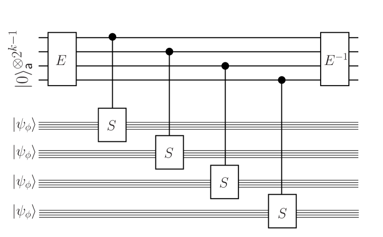
Figure 7: Parallelization of the PEA algorithm to estimate the bit $k=3$ of the phase. This replaces the outlined parts of the network in Fig. 6. $E$ is an entangler such that $E|0\rangle_{\sf a}^{\otimes 2^{k-1}}=({|}{0\cdots 0}{\rangle}_{\sf a}+{|}{1\cdots 1}{\rangle}_{\sf a})/\sqrt{2}$, and $E|100\cdots 0\rangle_{\sf a}=({|}{0\cdots 0}{\rangle}_{\sf a}-{|}{1\cdots 1}{\rangle}_{\sf a})/\sqrt{2}$. $E^{-1}$ is the decoding operation that maps $E^{-1}{|}{0\cdots 0}{\rangle}_{\sf a}={|}{+0\cdots 0}{\rangle}_{\sf a}$, and $E^{-1}{|}{1\cdots 1}{\rangle}_{\sf a}={|}{-0\cdots 0}{\rangle}_{\sf a}$, where ${|}{\pm}{\rangle}=({|}{0}{\rangle}\pm{|}{1}{\rangle})/\sqrt{2}$. The $k$’th bit is estimated from the measurement outcome of the first ancilla qubit in the logical basis.

Based on the discussion in the previous paragraph, the main obstacle to parallelizing the OEA is the preparation of ${|}{\psi_{\phi}}{\rangle}$. If $\phi=2\arccos(|\mbox{tr}(S\rho)|)$ is not close to $0$, ${|}{\psi_{\phi}}{\rangle}$ can be prepared near deterministically with relatively few resources as follows. Suppose we have a lower bound $\epsilon$ on $\phi$. With the original initial state, use sequential phase estimation with precision $\epsilon/2$ and confidence level $1-(1-c)p/B$ to determine whether we have projected onto the eigenstate ${|}{\psi_{\phi}}{\rangle}$ with eigenvalue $e^{i\phi}$ or the one with $e^{-i\phi}$. The occurrence of $p$ in the confidence level accounts for the total number of states that need to be prepared. The parameter $B$ is a constant that provides an additional adjustment to the confidence level. It must be chosen sufficiently large, and other confidence level parameters must be adjusted accordingly, to achieve the desired overall confidence level. If we have projected onto ${|}{\psi_{\phi}}{\rangle}$, return the state. If not, either try again, or adapt the parallel PEA to use the inverse operator $S^{\dagger}$ instead of $S$ for this instance of the initial state. The (sequential) resources required are of the order of $|\log((1-c)p)|/\epsilon$, but all the needed states can be prepared in parallel. For $\epsilon$ constant, the time required by the parallel PEA is increased by a factor of $O(|\log((1-c)p)|)$. The parallel overlap estimation for a unitary operator $U$ based on these variations of phase estimation thus requires $O(|\log((1-c)p)|)$ time, provided $|{\langle}{\psi}{|}U{|}{\psi}{\rangle}|$ is not too close to $1$.

For $|{\langle}{\psi}{|}U{|}{\psi}{\rangle}|$ close to $1$, the OEA is intrinsically not parallelizable without increasing the total resource cost by a factor of up to $O(\sqrt{p})$. This is due to the results in Zalka (1999), where it is shown that Grover’s algorithm cannot be parallelized without reducing the performance to that of classical search. For example, consider the problem of determining which unique state ${|}{k}{\rangle}$ of the states ${|}{0}{\rangle},\ldots{|}{2^{n}}{\rangle}$ has its sign flipped by a “black-box” unitary operator $V$. This can be done with $n$ many uses of the OEA by preparing the states ${|}{\psi_{b}}{\rangle}$ that are uniform superpositions of the ${|}{i}{\rangle}$ for which the number $i$ has $1$ as its $b$’th bit. If ${\langle}{\psi_{b}}{|}U{|}{\psi_{b}}{\rangle}=1/2^{n-1}$, then the $b$’th bit of $k$ is $1$. If ${\langle}{\psi_{b}}{|}U{|}{\psi_{b}}{\rangle}=0$, then it is $0$. It suffices to use an unparametrized (Fig. 4) precision of $1/2^{n-1}$ and confidence level sufficiently much bigger than $1-1/n$. Because $|1-\cos(\phi)|=O(\phi^{2})$, the parameterized precision required is $\Theta(1/2^{n/2})$. ($\Theta(x)$ is a quantity that is both $O(x)$ and $\Omega(x)$.) Thus $O(n2^{n/2})$ sequential resources suffice, which is close to the optimum attained by Grover’s algorithm. However, the results of Zalka (1999) imply that implementing quantum search with depth (sequential time) $d$ requires $\Omega(2^{n}/d)$ uses of $V$ for $d<2^{n/2}$. This implies that to achieve a parameterized precision of $\Theta(1/2^{n/2})$ for $1-|{\langle}{\psi}{|}U{|}{\psi}{\rangle}|=O(1/2^{n})$ using time $O(2^{n/2}/P)$ requires $\Omega(2^{n/2}P)$ resources.

The EEA was described so that overlap estimation is used with small $\phi$, and therefore can not be immediately parallelized without loss of precision or larger resource requirements. However, for the version of overlap estimation needed for stages I’ and II’, it is only the imaginary part of the overlap that is needed, and the parameters are chosen so that the overlap’s phase is expected to be within $1$ of $0$ (because $\theta_{\max}\leq 1$). The actual precision required is absolute in the overlap, not the parameterization of the overlap in terms of the upper hemisphere in Fig. 4. This implies that we can call the parallel overlap algorithm with an intentionally suppressed overlap. If the desired overlap is ${\langle}{\psi}{|}U{|}{\psi}{\rangle}$, one way to suppress it is to replace ${{U}^{({\mathsf{S}})}}$ by ${{{{}^{c}\!U}}^{({\mathsf{aS}})}}$ and the initial state by $({{\mathbf{I}}^{({\mathsf{a}})}}/2){|}{\psi}{\rangle}_{{}_{\!\!\scriptstyle{\mathsf{S}}}}\!\!{}^{\scriptstyle\mathsf{S}}\!{\langle}{\psi}{|}$. The suppression ensures that the phases in the calls to the PEA are sufficiently distinguishable to allow the near deterministic preparation of the appropriate eigenstates discussed above. This adds at most a constant overhead to the EEA due to the additional precision required to account for the scaling associated with the overlap suppression.