Photon wave functions and quantum interference experiments

Abstract

We present a general theory to describe two-photon interference, including a formal description of few photon intereference in terms of single-photon amplitudes. With this formalism, it is possible to describe both frequency entangled and separable two-photon interference in terms of single-photon wave functions. Using this description, we address issues related to the physical interpretation of two-photon interference experiments. We include a discussion on how few-photon interference can be interpreted as a bosonic exchange effect, and how this relates to traditional exchange effects with fermions.

Newton and WignerNW first discussed the non-localizability of photons, which prevents the introduction of a position-representation wave function in the usual sense of a wave function for a massive particle. Nonetheless, it has been known for years that it is possible to present physically meaningful descriptions of photon detection in finite regions of spaceMANDELETC . This has led to a host of approaches to introduce a “photon wave function” SIPEBIAL , each of which establishes at least a limited analogy to massive particle wave functions. Today there is no single accepted definition of such a photon wave function, as there are a variety of possible analogies, and the most convenient often depends on the system one would like to describe. For example, Chan et al. CHAN discuss a wave function associated with a photon spontaneously emitted from an atom in terms Schmidt pairs of atomic and photonic eigenfunctions, whereas Resch et al. RESCH find it useful to consider a photon wave function based on the Glauber detection probabilityMW in understanding an absorptive exchange effect. Given the variety of convenient types of “photon wave functions” introduced in the literature, it is perhaps best not to insist on a particular definition, but rather to understand the term to refer broadly to any approach for describing a photon in a manner analogous to the usual massive particle wavefunctions introduced in nonrelativistic physics. That is the point of view we take here, where we use photon wave functions to describe few-photon interference experiments. Although in the particulars of our discussion we use a photon wave function definition based on the Glauber detection formula, within the usually relevant approximations an easy translation into other photon wave function definitions could be made.

Yet one might ask, “why bother?” After all, the measurement results of two-photon interference experiments can be predicted with relatively simple, well-known calculations. Still, what seems to be a less straightforward task is the physical interpretation of the experiments. Few-photon interference is often discussed loosely in terms of interfering Feynman paths, or the overlap of wave packets, or the distinguishability of a particular set of outcomes. In this paper we formally address what one must mean if one wishes to discuss the interference of individual photon amplitudes leading to a particular detection event. Using photon wave functions, we explicitly show that second-order interference experiments can be understood in terms of single-photon amplitudes. Consequently, this approach yields considerable insight into few-photon interference experiments, and illustrates the relevance of the bosonic nature of the photonFEARN1 by contrasting the corresponding description that would result for fermions. It is with a photon wave function description that one can perhaps best isolate non-classical interference terms, and discuss the interference of single-photon amplitudes corresponding to a particular detection.

Perhaps the most familiar few-photon interference experiment involves the Hong-Ou-Mandel interferometerHOM . We show how second-order interference of this type manifests itself as an exchange effect in the photon wave function picture. This seems to be appreciated by many workers in the field, although we have not been able to find an explicit discussion of this point in the literature. We then move on to other experiments. We show how the elimination of which-path distinguishing information restores the exchange effect in quantum eraser experimentsQE . And while in their discussion of a postponed compensation experimentPITTMAN1 Pittman et al. emphasize the limitations of using a pair of photon wave packets to describe frequency entangled two-photon interference, we show that it is indeed possible to understand this experiment in terms of the interference of single photon amplitudes. Before proceeding to these issues in section II below, we identify our definition and notation for few-photon wave functions in section I; our conclusions are presented in section III.

I Photon wave functions

Photon wave functions can be extracted from the usual field theory description of photodetection, and used in a way similar to the use of massive particle wave functions in describing the detection of those particles. To establish this analogy we recall some well-known results from the field theory for nonrelativistic massive particles, in which an arbitrary single-particle state $\left|S\right\rangle$ can be written as

$$\left|S\right\rangle=\sum_{\lambda}g^{S}(\lambda)a^{\dagger}\left(\lambda\right)\left|vac\right\rangle,$$ (1)

where each $\lambda$ identifies one of a set of normalized, orthogonalized single-particle modes, $\left|vac\right\rangle$ is the vacuum state, and $a^{\dagger}\left(\lambda\right)$ is the associated particle creation operator. For particles in free space we can take $\lambda=(\mu,{\bf k})$ to label both the spin state $\mu$ and the wave vector ${\bf k}$ of a plane wave. Here $g^{S}(\lambda)$ is a normalized amplitude, satisfying

$$\sum_{\lambda}\left|g^{S}(\lambda)\right|^{2}=1.$$ (2)

We can write this state (1) in terms of the creation operator for a particle with spin label $\mu$ at ${\bf r}$,

$$\widehat{\Psi}_{\mu}^{\dagger}\left({\bf r}\right)=\frac{1}{\sqrt{V}}\sum_{{\bf k}}a^{\dagger}\left(\lambda\right)e^{i{\bf k\cdot r}}$$

where $V$ is a normalization volume, as

$$\left|S\right\rangle=\sum_{\mu}\int d{\bf r\,}G_{\mu}^{S}({\bf r})\widehat{\Psi}_{\mu}^{\dagger}\left({\bf r}\right)\left|vac\right\rangle,$$ (3)

where

$$G_{\mu}^{S}({\bf r})=\frac{1}{\sqrt{V}}\sum_{{\bf k}}g^{S}(\lambda)e^{i{\bf k\cdot r}},$$

and we anticipate the passage to the limit of infinite $V$ and the resulting continuous range of ${\bf k}$ over plane wave modes. We can now identify the single-particle wave function $\Phi_{\mu}^{S}({\bf r},t)$ associated with the single particle state $\left|S\right\rangle$. The state $\widehat{\Psi}_{\mu}\left({\bf r,}t\right)\left|S\right\rangle$, where $\widehat{\Psi}_{\mu}\left({\bf r,}t\right)=$ $\widehat{U}\left(t,0\right)\widehat{\Psi}_{\mu}\left({\bf r}\right)\widehat{U}^{\dagger}\left(t,0\right)$ and $\widehat{U}\left(t,0\right)$ is the time evolution operator from $0$ to $t$ determined by the Schrödinger equation, is proportional to the vacuum state; the wave usual function $\Phi_{\mu}^{S}({\bf r},t)$ of elementary quantum mechanics provides just that proportionality,

$$\widehat{\Psi}_{\mu}\left({\bf r,}t\right)\left|S\right\rangle=\Phi_{\mu}^{S}\left({\bf r,}t\right)\left|vac\right\rangle,$$ (4)

as can be easily confirmed. The probability of detecting the particle within $d{\bf r}$ of ${\bf r}$ at time $t$ can now be written in either the particle or field theory notation,

$$\sum_{\mu}\left|\Phi_{\mu}^{S}\left({\bf r,}t\right)\right|^{2}d{\bf r}=\sum_{\mu}\left\langle S\right|\widehat{\Psi}_{\mu}^{\dagger}\left({\bf r,}t\right)\widehat{\Psi}_{\mu}\left({\bf r,}t\right)\left|S\right\rangle\,d{\bf r}.$$ (5)

Moving to two-particle states, we can construct the most general such state $\left|T\right\rangle$ according to

$$\left|T\right\rangle=N^{T}\sum_{\lambda,\lambda^{\prime}}f^{T}\left(\lambda,\lambda^{\prime}\right)a^{\dagger}\left(\lambda\right)a^{\dagger}\left(\lambda^{\prime}\right)\left|vac\right\rangle=\sum_{\mu,\mu^{\prime}}\int\int d{\bf r}d{\bf r}^{\prime}F_{\mu\mu^{\prime}}^{T}\left({\bf r},{\bf r}^{\prime}\right)\widehat{\Psi}_{\mu}^{\dagger}\left({\bf r}\right)\widehat{\Psi}_{\mu^{\prime}}^{\dagger}\left({\bf r}^{\prime}\right)\left|vac\right\rangle,$$ (6)

where for later convenience we have introduced an explicit normalization constant $N^{T}$ such that $\left\langle T|T\right\rangle=1$, and

$$F_{\mu\mu^{\prime}}^{PQ}\left({\bf r},{\bf r}^{\prime}\right)=\frac{N^{T}}{V}\sum_{{\bf k,k}^{\prime}}f^{T}\left(\lambda,\lambda^{\prime}\right)e^{i{\bf k\cdot r}}e^{i{\bf k^{\prime}\cdot r}^{\prime}}.$$

Without loss of generality the amplitude $f^{T}\left(\lambda,\lambda^{\prime}\right)$ can be taken to be symmetric with respect to the interchange of $\lambda$ and $\lambda^{\prime}$ for bosons, and antisymmetric with respect to that interchange for fermions. A two-time, two-particle wave function (or bi-particle wave function), $\Phi_{\mu\mu^{\prime}}^{T}\left({\bf r},{\bf r}^{\prime},t,t^{\prime}\right)$, can be introduced according to

$$\frac{1}{\sqrt{2}}\widehat{\Psi}_{\mu}\left({\bf r,}t\right)\widehat{\Psi}_{\mu^{\prime}}\left({\bf r}^{\prime}{\bf,}t^{\prime}\right)\left|T\right\rangle=\Phi_{\mu\mu^{\prime}}^{T}\left({\bf r},{\bf r}^{\prime},t,t^{\prime}\right)\left|vac\right\rangle.$$ (7)

It is easy to show that $\Phi_{\mu\mu^{\prime}}^{T}({\bf r,r}^{\prime},t,t)$ is the usual two-particle wave function at time $t$, symmetric (or antisymmetric) with the interchange of $({\bf r,}\mu)$ and $({\bf r}^{\prime},\mu^{\prime})$, if we deal with bosons (or fermions). And considering detection processess activated at time $t$, a standard calculation easily done at the wave function level shows that the probability of detecting one particle within $d{\bf r}$ of ${\bf r}$ and a second particle within $d{\bf r}^{\prime}$ of ${\bf r}^{\prime}$ is given by GRAHAM

$$\sum_{\mu\mu^{\prime}}\left|\Phi_{\mu\mu^{\prime}}^{T}\left({\bf r},{\bf r}^{\prime},t,t\right)\right|^{2}d{\bf r}d{\bf r}^{\prime}=\frac{1}{2}\sum_{\mu\mu^{\prime}}\left\langle T\left|\widehat{\Psi}_{\mu^{\prime}}^{\dagger}\left({\bf r}^{\prime}{\bf,}t\right)\widehat{\Psi}_{\mu}^{\dagger}\left({\bf r,}t\right)\widehat{\Psi}_{\mu}\left({\bf r,}t\right)\widehat{\Psi}_{\mu^{\prime}}\left({\bf r}^{\prime}{\bf,}t\right)\right|T\right\rangle d{\bf r}d{\bf r}^{\prime}.$$ (8)

We now introduce photon wave functions in such a way that the equivalences (5,8) between wave functions and field theory descriptions hold when the standard Glauber detection formulas are used to model photodetection probabilities. Between detector activations we assume that the electromagnetic field evolves as a free radiation field. A modified version of this approach can be written down if this is not the case, but we will not do so here. We begin by introducing a single-photon state by analogy with (1),

$$\left|S\right\rangle=\sum_{\lambda}g^{S}(\lambda)a^{\dagger}\left(\lambda\right)\left|vac\right\rangle$$ (9)

where $a^{\dagger}\left(\lambda\right)$ is the photon creation operator for a mode $\lambda$, where the index $\lambda$ labels both the polarization (or helicity) and the wave vector ${\bf k}$, and the amplitudes $\left\{g^{S}(\lambda)\right\}$ again satisfy (2). The single-photon wave function at position ${\bf r}$ and time $t$, ${\bf\Phi}^{S}({\bf r,}t{\bf)}$ is defined by

$${\bf E}^{+}({\bf r},t)\left|S\right\rangle={\bf\Phi}^{S}({\bf r},t)\left|vac\right\rangle$$ (10)

where

$${\bf E}^{+}({\bf r},t) = i\sum_{\lambda}K_{k}\hat{e}_{\lambda}a\left(\lambda\right)e^{i({\bf k\cdot r}-\omega_{k}t)},$$ (11)

$${\bf E}^{-}({\bf r},t) = \left({\bf E}^{+}({\bf r},t)\right)^{\dagger}$$

are respectively the positive and negative frequency components of the electric field operator ${\bf E(r},t)=$ ${\bf E}^{+}({\bf r},t)+{\bf E}^{-}({\bf r},t),$ $K_{k}=\sqrt{2\pi\hbar\omega_{k}/V}$ with $V$ as the normalization volume, $\hat{e}_{\lambda}$ is the unit vector indicating the polarization, and $\omega_{k}=c\left|{\bf k}\right|$ is the angular frequency of wave vector ${\bf k}$. The analogy of this photon wave function with the single particle wave function of a nonrelativistic particle lies in the fact that, for the single photon state, the Glauber detection rate of a single ideal detector at position ${\bf r}$ and at time $t$ is proportional to the first order correlation function, given byMW

$$w^{(1)}({\bf r},t)=\left\langle S\right|{\bf E}^{-}({\bf r},t)\cdot{\bf E}^{+}({\bf r},t)\left|S\right\rangle=\left|{\bf\Phi}^{S}({\bf r},t)\right|^{2},$$ (12)

cf. (5). For photon wave functions this is, of course, not a fundamental postulate of the theory, but is derived from the Glauber detection model; in particular, we use a form of the model where the detector is assumed isotropic. The dynamics of ${\bf\Phi}^{S}({\bf r},t)$ are not governed by the Schrödinger equation, as in the massive particle case, but rather by Maxwell’s equations.

The analogy with massive particles carries on to states with more than one excitation. A general two-photon state of the radiation field is described by

$$\left|T\right\rangle=N^{T}\sum_{\lambda,\lambda^{\prime}}f^{T}\left(\lambda,\lambda^{\prime}\right)a^{\dagger}\left(\lambda\right)a^{\dagger}\left(\lambda^{\prime}\right)\left|vac\right\rangle$$ (13)

where $N^{T}$ is the normalization factor, which for photons (or massive bosons) can be taken to be

$$N^{T}=\left(\sum_{\lambda,\lambda^{\prime}}\left|f^{T}\left(\lambda,\lambda^{\prime}\right)\right|^{2}+\sum_{\lambda,\lambda^{\prime}}\left[f^{T}\left(\lambda^{\prime},\lambda\right)\right]^{\ast}f^{T}\left(\lambda,\lambda^{\prime}\right)\right)^{-\frac{1}{2}},$$ (14)

to guarantee $\left\langle T|T\right\rangle=1.$ We do not choose the function $f^{T}$ itself to be normalized, as it is convenient to write the normalization factor separately when comparing two-photon states to corresponding single-photon states. A special case is that for which the amplitude $f^{T}\left(\lambda,\lambda^{\prime}\right)$ in some basis (taken here to be that of polarizations or helicities and wave vectors) can be written as the symmetric product of a function of $\lambda$ and a function of $\lambda^{\prime}$. Each of these functions can then be associated with a one-photon state. In such a case we write $f^{T}(\lambda,\lambda^{\prime})$ as the function $f^{PQ}\left(\lambda,\lambda^{\prime}\right)=g^{P}(\lambda)g^{Q}(\lambda^{\prime})+g^{P}(\lambda^{\prime})g^{Q}(\lambda),$ where $\left\{g^{P}(\lambda)\right\}$ and $\left\{g^{Q}(\lambda)\right\}$ are normalized spectral amplitudes (2) associated with single photon states, and we call the two-photon state separable. As is usually done in the literature, one can describe the same state with the simpler non-symmetric function $f^{PQ}\left(\lambda,\lambda^{\prime}\right)=g^{P}(\lambda)g^{Q}(\lambda^{\prime})$ since the additional component does not change the state (13).  With this choice of $f^{PQ}\left(\lambda,\lambda^{\prime}\right)$, for such separable states,

$$N^{PQ}=\left(1+\left|\sum_{\lambda}\left[g^{P}(\lambda)\right]^{*}g^{Q}(\lambda)\right|^{2}\right)^{-\frac{1}{2}},$$ (15)

and $N^{PQ}=1$ only if the two single photon amplitudes are orthogonal; if $P=Q$ we have a state of two identical photons, and $N^{PQ}=2^{-1/2}$.

We introduce a two-photon wave function (sometimes called a biphotonRUBIN1 ) that satisfies

$$\frac{1}{\sqrt{2}}E_{j}^{+}({\bf r}_{2},t_{2})E_{i}^{+}({\bf r}_{1},t_{1})\left|T\right\rangle=\Phi_{{}_{ij}}^{T}({\bf r}_{1},{\bf r}_{2},t_{1},t_{2})\left|vac\right\rangle,$$ (16)

where Roman subscripts denote Cartesian components, and $\Phi_{{}_{ij}}^{T}({\bf r}_{1},{\bf r}_{2},t_{1},t_{2})$ are the components of the wave function associated with the state $\left|T\right\rangle$. In a general two-photon state, the coincidence detection rate of two ideal detectors at positions ${\bf r}_{1}$, ${\bf r}_{2}$ and at times $t_{1}$, $t_{2}$ is proportional to the second order correlation functionMW

$$w^{\left(2\right)}({\bf r}_{1},{\bf r}_{2},t_{1},t_{2}) = \sum_{ij}\left\langle T\left|E_{i}^{-}({\bf r}_{1},t_{1})E_{j}^{-}({\bf r}_{2},t_{2})E_{j}^{+}({\bf r}_{2},t_{2})E_{i}^{+}({\bf r}_{1},t_{1})\right|T\right\rangle$$

$$= 2\sum_{ij}\left|\Phi_{{}_{ij}}^{T}({\bf r}_{1},{\bf r}_{2},t_{1},t_{2})\right|^{2},$$

cf. (8), where $\Phi_{ij}^{T}({\bf r}_{1},{\bf r}_{2},t_{1},t_{2})$ is symmetric under exchange of $(i,{\bf r}_{1},t_{1})$ with $(j,{\bf r}_{2},t_{2})$.

II Interference experiments

We now examine a type of quantum interference, observed in a number of few-photon experiments, that is associated with the measurement of particular coincidence detection rates. We discuss these rates in terms of interfering single-photon amplitudes, and show that the interference can be associated with photon exchange effects.

The simplest type of two-photon state is a separable one, in which we can write $f^{PQ}\left(\lambda,\lambda^{\prime}\right)=g^{P}(\lambda)g^{Q}(\lambda^{\prime})$. Here we can say that one photon has the spectral properties of ‘Photon $P$’ and one photon has the properties of ‘Photon $Q$’ referring to the single-photon states $\left|P\right\rangle$ and $\left|Q\right\rangle$. For massive fermions, the analogous kind of separable spectral amplitude corresponds to a standard Hartree-Fock, single-determinant wave function. In many-body physics one usually characterizes such a state as free of the “correlation effects” that arise due to electron-electron interactions in more sophisticated models of the full, many-electron wave function. Nonetheless, there are dynamical consequences due to exchange effects even in separable states, which arise for bosons as well, and in particular photons. After considering the separable case, we generalize the discussion to address frequency entangled few-photon interference experiments that explicitly involve correlation effects.

The two-photon wave function for a separable two-photon state takes the form

$$\Phi_{{}_{ij}}({\bf r}_{1},{\bf r}_{2},t_{1},t_{2})=\frac{N^{PQ}}{\sqrt{2}}\left[\Phi_{{}_{i}}^{P}({\bf r}_{1},t_{1})\Phi_{{}_{j}}^{Q}({\bf r}_{2},t_{2})+\Phi_{{}_{i}}^{Q}({\bf r}_{1},t_{1})\Phi_{{}_{j}}^{P}({\bf r}_{2},t_{2})\right],$$ (18)

with the $+$ arising instead of a $-$ because photons are bosons, and where $\Phi_{i}^{P}({\bf r},t)$ and $\Phi_{j}^{Q}({\bf r},t)$ are the single-particle wave functions associated with photons $P$ and $Q$ respectively. It is in this form that one can discuss interference in terms of individual photon amplitudes. The second-order correlation function is

$$w^{\left(2\right)}({\bf r}_{1},{\bf r}_{2},t_{1},t_{2}) = \sum_{ij}\left|N^{PQ}\right|^{2}\bigg{[}\left|\Phi_{{}_{i}}^{P}({\bf r}_{1},t_{1})\right|^{2}\left|\Phi_{{}_{j}}^{Q}({\bf r}_{2},t_{2})\right|^{2}+\left|\Phi_{{}_{j}}^{Q}({\bf r}_{1},t_{1})\right|^{2}\left|\Phi_{{}_{i}}^{P}({\bf r}_{2},t_{2})\right|^{2}$$

$${}+\left[\Phi_{{}_{i}}^{P}({\bf r}_{1},t_{1})\right]^{\ast}\Phi_{{}_{i}}^{Q}({\bf r}_{1},t_{1})\left[\Phi_{{}_{j}}^{Q}({\bf r}_{2},t_{2})\right]^{\ast}\Phi_{{}_{j}}^{P}({\bf r}_{2},t_{2})$$

$${}+\left[\Phi_{{}_{i}}^{Q}({\bf r}_{1},t_{1})\right]^{\ast}\Phi_{{}_{i}}^{P}({\bf r}_{1},t_{1})\left[\Phi_{{}_{j}}^{Q}({\bf r}_{2},t_{2})\right]^{\ast}\Phi_{{}_{j}}^{Q}({\bf r}_{2},t_{2}){}\bigg{]}.$$

The first two terms on the right-hand side of (II) are the classical independent-particle terms. If only these terms were present, the detection coincidence would be simply identified with the alternatives “photon $P$ at $({\bf r}_{1},t_{1})$ and photon $Q$ at $({\bf r}_{2},t_{2})$” or “photon $Q$ at $({\bf r}_{1},t_{1})$ and photon $P$ at $({\bf r}_{2},t_{2})$” characteristic of independent detection events. The last two terms on the right-hand side are the interference or exchange terms. One can see that the exchange terms are proportional to the indistinguishability, or overlap, of the $P$ and $Q$ single-photon amplitudes in the region of interest. Non-zero exchange terms are indicative of the “indistinguishable Feynman paths” or “overlapping single-photon amplitudes” sometimes mentioned in the few-photon literature.

It is important to consider the finite detection window of a realistic detector. Though the exchange terms in (II) may be non-zero for some values of $t_{1}$ and $t_{2}$, the exchange terms may integrate to zero over a finite detection time. Particularity if one were to consider photons in different frequency ranges, one would find that spatially overlapping single-photon amplitudes would give rise to instantaneously non-zero exchange terms that would integrate to zero over a realistic detection time. It would be possible to observe interference between photons in different frequency ranges provided that the detection window were sufficiently short, but in practice no interference would be observed regardless of the spatial configuration of the photon wavefunctions in the region of detection. In contrast, if the photons have the same peak frequency, the spatial overlap of single-photon amplitudes in the detection region is sufficient to give rise to exchange terms that do not integrate to zero over a realistic detection time. In the subsequent discussion we assume that we are dealing with photons that have the same peak frequency, and thus where there are overlapping single-photon amplitudes in the detection region there are exchange effects in coincidence measurements.

We now apply this formalism to several important two-photon interference experiments, and demonstrate that in each case the interference can be understood as single-photon wave function amplitudes giving rise to an exchange effect.

II.1 The Hong-Ou-Mandel interferometer

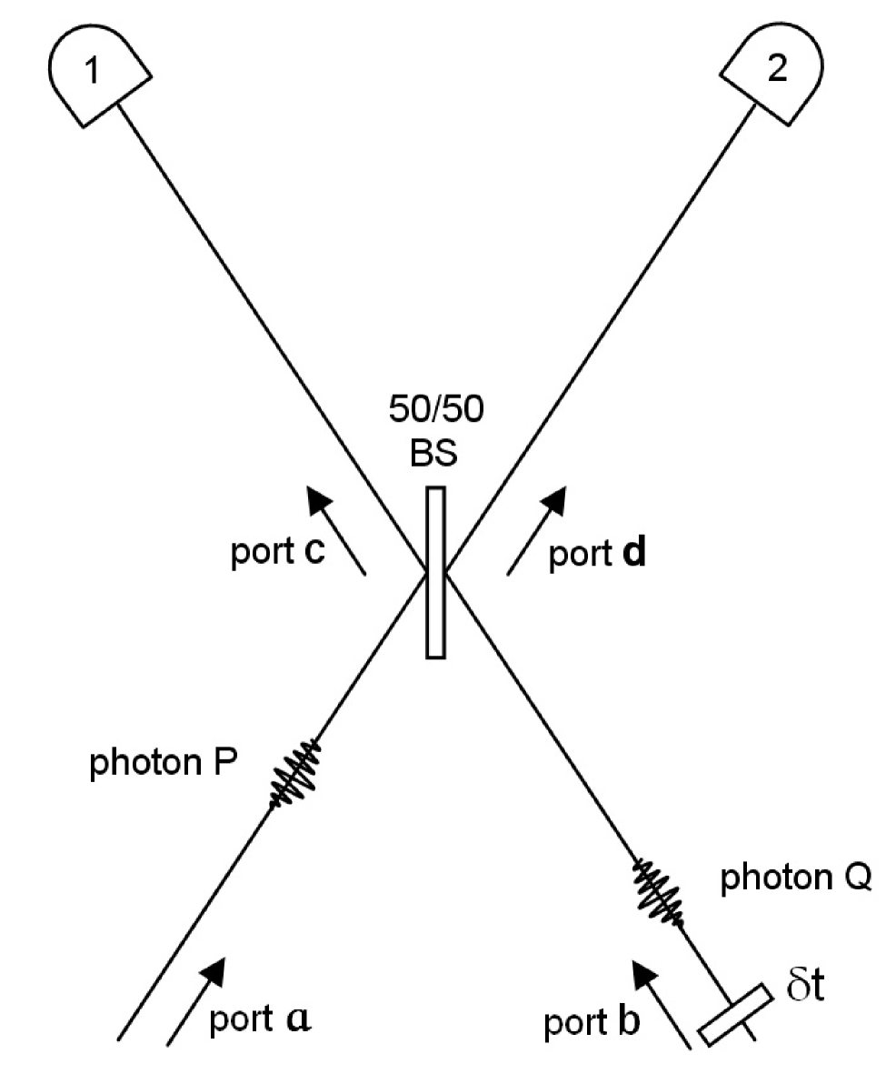
Figure 1: A schematic diagram of the Hong-Ou-Mandel interferometer. Two like-polarized photons are incident on a beam splitter. The arrival of the photon in port $b$ is delayed by $\delta t$. Interference is observed in the coincidence detection rate of the two detectors. The origins of ports $c$ and $d$ are at the beam splitter, while the origins of ports $a$ and $b$ are at distance $c\Delta$ behind the beam splitter.

First we consider the simple case of the Hong-Ou-Mandel interferometer. A schematic diagram of this experiment is shown in Fig. 1, where we label the input ports $a$ and $b$, and the output ports $c$ and $d$. Two photons are incident on the 50/50 beam splitter, with one of the photons delayed in time by $\delta t$. We use a simplified notation, taking only one linear polarization associated with each port, and considering small wave packets with a narrow spread of wave vector components perpendicular to the direction identified by the port. Hence a one-dimensional treatment is possible for each port. We use, for example, $a_{b}^{\dagger}\left(k\right)$ to denote a creation operator associated with a wave vector of magnitude $k$ and in the propagation direction relevant for port $b$. In this shorthand the initial separable two-photon state, at a time just before the photon wave functions impinge on the beam-splitter, can be written as

$$\left|P_{a},Q_{b}\right\rangle=\int\int dkdk^{\prime}g^{P}(k)g^{Q}(k^{\prime})a_{a}^{\dagger}\left(k\right)a_{b}^{\dagger}\left(k^{\prime}\right)\left|vac\right\rangle,$$ (20)

where we have gone to a continuous range of wave numbers. In the full notation used in the previous section the functions $g^{P}({\bf k})$ and $g^{Q}({\bf k})$ would of course be orthogonal, since the single-photon wave functions do not overlap. But in our shorthand notation we take photons $P_{a}$ and $Q_{b}$ to be the same when referenced to their own ports, with only the second delayed by a time $\delta t$ from the first; thus $g^{Q}(k)=g^{P}(k)e^{i\omega_{k}\delta t}$. In order to reduce the calculation to simple integration over one-dimensional coordinates we use the scalars, $x_{n}$, and mode indices, $j_{n}$, where $x_{n}$ is the spatial coordinate for the input port $j_{n}$, together to identify a position ${\bf r}$ of interest. With this notation and Eq. (20) the two-photon wave function in the region just before the beam splitter can be written as

$$\Phi(j_{1},x_{1};j_{2},x_{2};t_{1},t_{2})=\frac{1}{\sqrt{2}}\left[\Phi^{P}(j_{1},x_{1};t_{1})\Phi^{Q}(j_{2},x_{2};t_{2})+\Phi^{Q}(j_{1},x_{1};t_{1})\Phi^{P}(j_{2},x_{2};t_{2})\right],$$ (21)

where the single-photon wavefunction $\Phi^{P}(j,x;t)$ is defined by the obvious simplification of (10) and

$$\Phi^{P}(a,x;t) = \int dkg^{P}(k)e^{i(kx-\omega_{k}t)}=V^{P}(x,t),$$ (22)

$$\Phi^{Q}(b,x;t) = \int dkg^{Q}(k)e^{i(kx-\omega_{k}t)}=V^{Q}(x,t),$$

$$\Phi^{P}(b,x;t) = \Phi^{Q}(a,x;t)=0.$$

The origins of ports $a$ and $b$ are equally distant from the beam splitter, as shown in Fig. 1. We have given the one-dimensional single-photon wave functions in this input region a special label, $V^{P(Q)}(x,t),$ so that we can illustrate how these input wave functions interfere in the detection region. The wave function amplitude corresponding to a two-photon detection event in the input region before the beam splitter is

$$\Phi(a,x_{1};b,x_{2};t_{1},t_{2}) = \Phi(b,x_{2};a,x_{1};t_{2},t_{1})=\frac{1}{\sqrt{2}}\left[V^{P}(x_{1},t_{1})V^{Q}(x_{2},t_{2})\right]$$

$$= \frac{1}{\sqrt{2}}\left[V^{P}(x_{1},t_{1})V^{P}(x_{2},t_{2}-\delta t)\right]$$

and, as one would expect, the square modulus of this function does not give rise to exchange terms and there is no interference in this region. We now wish to evaluate the two-photon detection rate in the output ports $c$ and $d$; the origin of each of these ports is taken at the beam splitter. As is well known, the effect of the beam splitter is to effect a canonical transformation on the port operatorsBACHOR1 ,

$$a_{a}^{\dagger}\left(k\right) \rightarrow \frac{e^{i\omega_{k}\Delta}}{\sqrt{2}}\left[a_{d}^{\dagger}\left(k\right)-ia_{c}^{\dagger}\left(k\right)\right]$$ (24)

$$a_{b}^{\dagger}\left(k\right) \rightarrow \frac{e^{i\omega_{k}\Delta}}{\sqrt{2}}\left[a_{c}^{\dagger}\left(k\right)-ia_{d}^{\dagger}\left(k\right)\right],$$

where $\Delta$ is the time required for light to travel from the origins associated with ports $(a,b)$ to the beam-splitter, and it will be convenient below to use delayed time coordinates $\overline{t}_{1(2)}=t_{1(2)}-\Delta$. The two-photon wave function in the region of the detectors has the following components

$$\Phi(c,x_{1};c,x_{2};t_{1},t_{2}) = \frac{1}{2\sqrt{2}}\left[\Phi^{P}(c,x_{1};\overline{t}_{1})\Phi^{Q}(c,x_{2};\overline{t}_{2})+\Phi^{Q}(c,x_{1};\overline{t}_{1})\Phi^{P}(c,x_{2};\overline{t}_{2})\right]$$

$$\Phi(d,x_{1};d,x_{2};t_{1},t_{2}) = \frac{1}{2\sqrt{2}}\left[\Phi^{P}(d,x_{1};\overline{t}_{1})\Phi^{Q}(d,x_{2};\overline{t}_{2})+\Phi^{Q}(d,x_{1};\overline{t}_{1})\Phi^{P}(d,x_{2};\overline{t}_{2})\right]$$ (25)

$$\Phi(c,x_{1};d,x_{2};t_{1},t_{2}) = \Phi(d,x_{2};c,x_{1};t_{2},t_{1})=\frac{1}{2\sqrt{2}}\left[\Phi^{P}(c,x_{1};\overline{t}_{1})\Phi^{Q}(d,x_{2};\overline{t}_{2})+\Phi^{Q}(c,x_{1};\overline{t}_{1})\Phi^{P}(d,x_{2};\overline{t}_{2})\right].$$

We can write the wave function in terms of the single-photon input amplitude since

$$\Phi^{P}(c,x;t) = -iV^{P}(x,t)$$

$$\Phi^{P}(d,x;t) = V^{P}(x,t)$$ (26)

$$\Phi^{Q}(c,x;t) = V^{Q}(x,t)=V^{P}(x,t-\delta t)$$

$$\Phi^{Q}(d,x;t) = -iV^{Q}(x,t)=-iV^{P}(x,t-\delta t)$$

and we have

$$\Phi(c,x_{1};c,x_{2};t_{1},t_{2}) = \Phi(d,x_{1};d,x_{2};t_{1},t_{2})=\frac{-i}{2\sqrt{2}}\left[V^{Q}(x_{1},\overline{t}_{1})V^{P}(x_{2},\overline{t}_{2})+V^{P}(x_{1},\overline{t}_{1})V^{Q}(x_{2},\overline{t}_{2})\right]$$ (27)

$$\Phi(c,x_{1};d,x_{2};t_{1},t_{2}) = \Phi(d,x_{2};c,x_{1};t_{2},t_{1})=\frac{1}{2\sqrt{2}}\left[V^{Q}(x_{1},\overline{t}_{1})V^{P}(x_{2},\overline{t}_{2})-V^{P}(x_{1},\overline{t}_{1})V^{Q}(x_{2},\overline{t}_{2})\right].$$ (28)

One can see how the input amplitudes for the individual photons interfere when the two-photon wave function is written in terms of the input wave functions. As per the usual discussion, each photon is either reflected or transmitted by the beam splitter giving four possible “outcomes”. For each outcome there is a corresponding wave function component in equations (27)-(28). The $\Phi(c,x_{1};c,x_{2};t_{1},t_{2})$ and $\Phi(d,x_{1};d,x_{2};t_{1},t_{2})$ components are the amplitudes for a detection event when both detectors are in the same output port.  The amplitudes in (28) are those relevant to this experiment since we are interested in the coincidence detection rate where one photon is detected in each output port. The negative sign in (28) is the important feature that allows for destructive interference. A $-i$ phase shift occurs when a photon wavefunction is reflected and the amplitude corresponding to a detection where both photons are reflected by the beam splitter accumulates a $\pi$ phase shift relative to the amplitude of both photons being transmitted. The coincidence detection rate of the detectors is then proportional to

$$\left|\Phi(c,x_{1};d,x_{2};t_{1},t_{2})\right|^{2} = \frac{1}{8}\bigg{[}\left|V^{P}(x_{1},\overline{t}_{1})\right|^{2}\left|V^{P}(x_{2},\overline{t}_{2}-\delta t)\right|^{2}+\left|V^{P}(x_{1},\overline{t}_{1}-\delta t)\right|^{2}\left|V^{P}(x_{2},\overline{t}_{2})\right|^{2}$$

$${}-V^{P}(x_{1},\overline{t}_{1})\left[V^{P}(x_{1},\overline{t}_{1}-\delta t)\right]^{\ast}V^{P}(x_{2},\overline{t}_{2}-\delta t)\left[V^{P}(x_{2},\overline{t}_{2})\right]^{\ast}$$

$${}-\left[V^{P}(x_{1},\overline{t}_{1})\right]^{\ast}V^{P}(x_{1},\overline{t}_{1}-\delta t)\left[V^{P}(x_{2},\overline{t}_{2}-\delta t)\right]^{\ast}V^{P}(x_{2},\overline{t}_{2})\bigg{]}{}.$$

The last two terms of Eq. (II.1) are the exchange terms corresponding to the second two terms of (II). As the $P$ and $Q$ (delayed) photon amplitudes overlap in the detection region, the exchange terms bring the detection rate to zero. At zero delay there is maximum interference and the coincidence detection rate is zero: The exchange terms completely cancel out the classical independent-particle amplitude for a two-photon detection.  Similarily, evaluating

$$\left|\Phi(c,x_{1};c,x_{2};t_{1},t_{2})\right|^{2} = \frac{1}{8}\bigg{[}\left|V^{P}(x_{1},\overline{t}_{1})\right|^{2}\left|V^{P}(x_{2},\overline{t}_{2}-\delta t)\right|^{2}+\left|V^{P}(x_{1},\overline{t}_{1}-\delta t)\right|^{2}\left|V^{P}(x_{2},\overline{t}_{2})\right|^{2}$$

$${}+V^{P}(x_{1},\overline{t}_{1})\left[V^{P}(x_{1},\overline{t}_{1}-\delta t)\right]^{\ast}V^{P}(x_{2},\overline{t}_{2}-\delta t)\left[V^{P}(x_{2},\overline{t}_{2})\right]^{\ast}$$

$${}+\left[V^{P}(x_{1},\overline{t}_{1})\right]^{\ast}V^{P}(x_{1},\overline{t}_{1}-\delta t)\left[V^{P}(x_{2},\overline{t}_{2}-\delta t)\right]^{\ast}V^{P}(x_{2},\overline{t}_{2})\bigg{]}{}$$

shows the constructive interference exchange effect that arises when measuring the coincidence detection rate of two detectors in the same output port.  Assuming the photons are of finite temporal width, for large delay $\delta t$ we find $\left|\Phi(c,x_{1};c,x_{2};t_{1},t_{2})\right|^{2}=\left|\Phi(c,x_{1};d,x_{2};t_{1},t_{2})\right|^{2}.$ This may at first sight be surprising. According to the beam splitter transformations, each photon has a probability of $0.5$ of being detected in port $c$, and a probability of $0.5$ of being detected in port $d$. Since for large $\delta t$ we expect the photons to be independent, this would lead to a probability of $0.5$ that the photons are detected in separate exit ports, and a probability of only $0.25$ that they would both be detected in port $c$, for example. However, it is important to recall that we have based the theory on the Glauber detection model where it is assumed that the interaction between the radiation field and detector is weak. When two detectors are located in the same port this allows for each photon in that port to interact with both detectors, in some sense double-counting the photons.  This is the standard result of calculations based on the Glauber detection model.

We now expand the discussion to include the non-separable case, where we allow for the possibility of “frequency entanglement”. In the frequency entangled case Eq. (18) does not apply, and one cannot separately address the amplitudes of individual photons as previously discussed. Nonetheless, the photon wave function formalism can be used to describe frequency entangled two-photon interference in a slightly different way. Consider a two-port single-polarization gaussian entangled two-photon state as an input for the Hong-Ou-Mandel interferometer:

$$\left|P_{a},Q_{b}\right\rangle_{C} = N\left(\sigma\right)\int\int dkdk^{\prime}g^{P}(k)g^{Q}(k^{\prime})e^{-\frac{\left(\omega_{k}+\omega_{k^{\prime}}-2\omega_{k_{o}}\right)^{2}}{\sigma^{2}}}a_{a}^{\dagger}\left(k\right)a_{b}^{\dagger}\left(k^{\prime}\right)\left|vac\right\rangle$$ (31)

$$= N\left(\sigma\right)\frac{\sigma}{2\sqrt{\pi}}\int dte^{-\frac{\sigma^{2}t^{2}}{4}}e^{-2i\omega_{k_{o}}t}\left|\Psi\left(t\right)\right\rangle$$ (32)

where $\sigma$ is the entanglement width,

$$\left|\Psi\left(t\right)\right\rangle = \int\int dkdk^{\prime}g^{P}(k)e^{i\omega_{k}t}g^{Q}(k^{\prime})e^{i\omega_{k^{\prime}}t}a_{a}^{\dagger}\left(k\right)a_{b}^{\dagger}\left(k^{\prime}\right)\left|vac\right\rangle,$$ (33)

$$N\left(\sigma\right) = \left[\int\int dkdk^{\prime}\left|g^{P}(k)\right|^{2}\left|g^{Q}(k^{\prime})\right|^{2}e^{-\frac{2\left(\omega_{k}+\omega_{k^{\prime}}-2\omega_{k_{o}}\right)^{2}}{\sigma^{2}}}\right]^{-\frac{1}{2}},$$ (34)

and $2\omega_{k_{o}}$ is the peak entanglement angular frequency. One can think of this state as a superposition of separable two-photon states (33), each with the two photons temporally displaced by a time $t$. In the superposition (32) the amplitude of each component contain a phase factor that varies rapidly with this displacement time. The degree of the frequency entanglement determines the weighted distribution of these single-photon wave functions in time. It is in this form that one can discuss frequency entangled two-photon interference in terms of separable single-photon amplitudes.

For the Hong-Ou-Mandel experiment with frequency entangled photons, one can describe the interference in terms of the separable input wave function amplitudes with a superposition of two-photon wave functions distributed in time. The two-photon detection amplitude becomes

$$\Phi(c,x_{1};d,x_{2};t_{1},t_{2})=\frac{1}{4\sqrt{2}}N\left(\sigma\right)\frac{\sigma}{\sqrt{\pi}}\int e^{-\frac{\sigma^{2}t^{2}}{4}}e^{-2i\omega_{k_{o}}t}dt\left[V^{P}(x_{1},\overline{t}_{1}-t)V^{Q}(x_{2},\overline{t}_{2}-t)-V^{Q}(x_{1},\overline{t}_{1}-t)V^{P}(x_{2},\overline{t}_{2}-t)\right].$$ (35)

Comparing with (28) one can see that the phase shift of the reflected single-photon amplitudes once again allow for destructive interference. The detection rate is proportional to

$$\left|\Phi(c,x_{1};d,x_{2};t_{1},t_{2})\right|^{2} = \frac{1}{32}\left|N\left(\sigma\right)\right|^{2}\frac{\sigma^{2}}{\pi}\int\int e^{-\frac{\sigma^{2}\left(t+T\right)^{2}}{4}}e^{-2i\omega_{k_{o}}\left(t-T\right)}dtdT$$

$$\bigg{[}\left[V^{P}(x_{1},\overline{t}_{1}-t)\right]^{\ast}V^{P}(x_{1},\overline{t}_{1}-T)\left[V^{Q}(x_{2},\overline{t}_{2}-t)\right]^{\ast}V^{Q}(x_{2},\overline{t}_{2}-T)$$

$$+\left[V^{P}(x_{2},\overline{t}_{2}-t)\right]^{\ast}V^{P}(x_{2},\overline{t}_{2}-T)\left[V^{Q}(x_{1},\overline{t}_{1}-t)\right]^{\ast}V^{Q}(x_{1},\overline{t}_{1}-T)$$

$$-\left[V^{P}(x_{1},\overline{t}_{1}-t)\right]^{\ast}V^{Q}(x_{1},\overline{t}_{1}-T)\left[V^{Q}(x_{2},\overline{t}_{2}-t)\right]^{\ast}V^{P}(x_{2},\overline{t}_{2}-T)$$

$${}-V^{P}(x_{1},\overline{t}_{1}-T)\left[V^{Q}(x_{1},\overline{t}_{1}-t)\right]^{\ast}V^{Q}(x_{2},\overline{t}_{2}-T)\left[V^{P}(x_{2},\overline{t}_{2}-t)\right]^{\ast}\bigg{]}{}.$$

Here we have the possibility of exchange interference between amplitudes at different temporal displacements. Using this form it is possible to investigate the effect of frequency-entanglement on few-photon interference by examining the exchange terms. We will show that for a Hong-Ou-Mandel interferometer with a large enough delay such that the exchange terms are zero (no interference) with separable input photons, no amount of frequency-entanglement can introduce interference. We will begin with the assumption that the input wave functions can be well approximated as having finite temporal width, that is, if $\left|a\right|>\beta$ then $V^{P}(x,t)V^{P}(x,t+a)=0,$ where $\beta$ is a photon width parameter. Given $\left|\delta t\right|>\beta$, the exchange terms in (II.1) are zero and there is no interference in the separable case. To show that in this case there is no interference between temporally displaced two-photon wavefunctions, from examining the exchange terms in (II.1) we see we must show that for all $(t,T)$

$$\left[V^{P}(x_{1},t_{1}+t)\right]^{\ast}V^{P}(x_{1},t_{1}+\delta t+T)\left[V^{P}(x_{2},t_{2}+\delta t+t)\right]^{\ast}V^{P}(x_{2},t_{2}+T)=0.$$ (37)

The proof is by contradiction. First we suppose that Eq. (37) is does not hold.  With the finite temporal width assumption, this implies both $\left|\delta t+(T-t)\right|<\beta$ and $\left|\delta t-(T-t)\right|<\beta.$ But this is impossible to satisfy since $\left|\delta t\right|>\beta$. Hence (37) must hold and regardless of the entanglement, the exchange terms are zero if the initial relative photon delay, $\delta t$, is larger than temporal width of the single-photon wave functions. One can see this in Fig. 2, which shows a pictorial representation of the exchange terms in (II.1). In order for the exchange terms to contribute to the coincidence detection rate, all four single-photon wave functions must overlap at some value of $(t,T)$. Regardless of the temporal displacements, the single photon amplitudes in the exchange terms do not overlap for $\delta t$ larger than temporal width of the photon wave functions. We will discuss later how this is not the case for the postponed compensation experiment, where the frequency-entanglement is more significant.

II.2 Quantum eraser experiments

The version of the quantum eraserSCULLY1 we discuss here illustrates how the photon wave function formalism deals with multiple polarizations. The basic idea of the two-photon quantum eraser is as follows: It is possible to introduce distinguishing information in the input of an interferometer that would destroy second-order interference if the information were not “erased” at some stage before detectionQE . In our context, erasing distinguishing information is equivalent to producing overlapping wave functions in the detection region.

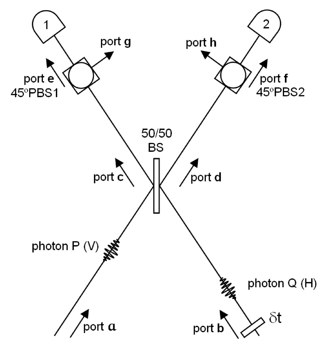
Figure 3: A schematic diagram of a quantum eraser. Orthogonally polarized photons are incident on a beam splitter. Interference in the coincidence detection rate is observed only in the region beyond the polarizing beam splitters PBS1 and PBS2.

Fig. 3 is a schematic diagram of a basic quantum eraser interferometer. Two orthogonally polarized photons in ports (a,b) interact with a beam splitter similar to the Hong-Ou-Mandel scenario. Since the photons are orthogonally polarized, it is possible to distinguish the final states of the two paths leading to a coincidence detection in ports c and d. It is the presence of the 45 degree polarizing beam splitters in front of the detectors that causes the distinguishing information to be destroyed so that second-order interference can occur. The input state is described by

$$\left|P_{aH},Q_{bV}\right\rangle=\int\int dkdk^{\prime}g^{P}(k)g^{Q}(k^{\prime})a_{aH}^{\dagger}\left(k\right)a_{bV}^{\dagger}\left(k^{\prime}\right)\left|vac\right\rangle$$ (38)

where, for example, $a_{aH}^{\dagger}\left(k\right)$ denotes a creation operator associated with a horizontally polarized photon of wave vector magnitude $k$ in the propagation direction relevant for port $a$. As in the previous subsection, we define the input region wave functions. The two-photon wave function in the region just before the beam splitter has two components:

$$\Phi_{HV}(a,x_{1};b,x_{2};t_{1},t_{2})=\Phi_{VH}(b,x_{2};a,x_{1};t_{2},t_{1})=\frac{1}{\sqrt{2}}V^{P}(x_{1},t_{1})V^{Q}(x_{2},t_{2}),$$

cf. (II.1). Once again the relevant action of the beam splitter maps the input ports ($a$,$b$) to the output ports ($c$,$d$) in the following way:

$$a_{aH}^{\dagger}\left(k\right) \rightarrow \frac{e^{i\omega_{k}\Delta}}{\sqrt{2}}\left[a_{dH}^{\dagger}\left(k\right)-ia_{cH}^{\dagger}\left(k\right)\right]$$ (39)

$$a_{bV}^{\dagger}\left(k\right) \rightarrow \frac{e^{i\omega_{k}\Delta}}{\sqrt{2}}\left[a_{cV}^{\dagger}\left(k\right)-ia_{dV}^{\dagger}\left(k\right)\right].$$

The components of the two-photon wavefunction just beyond the beam splitter are:

$$\Phi_{HV}(d,x_{1};d,x_{2};t_{1},t_{2}) = \Phi_{VH}(d,x_{2};d,x_{1};t_{2},t_{1})=-\frac{i}{2\sqrt{2}}V^{P}(x_{1},\overline{t}_{1})V^{Q}(x_{2},\overline{t}_{2})$$

$$\Phi_{HV}(c,x_{1};c,x_{2};t_{1},t_{2}) = \Phi_{VH}(c,x_{2};c,x_{1};t_{2},t_{1})=-\frac{i}{2\sqrt{2}}V^{P}(x_{1},\overline{t}_{1})V^{Q}(x_{2},\overline{t}_{2})$$ (40)

$$\Phi_{HV}(c,x_{1};d,x_{2};t_{1},t_{2}) = \Phi_{VH}(d,x_{2};c,x_{1};t_{2},t_{1})=-\frac{1}{2\sqrt{2}}V^{P}(x_{1},\overline{t}_{1})V^{Q}(x_{2},\overline{t}_{2})$$

$$\Phi_{VH}(c,x_{1};d,x_{2};t_{1},t_{2}) = \Phi_{HV}(d,x_{2};c,x_{1};t_{2},t_{1})=\frac{1}{2\sqrt{2}}V^{Q}(x_{1},\overline{t}_{1})V^{P}(x_{2},\overline{t}_{2}),$$

cf. (25). To demonstrate that it is indeed the presence of the 45 degree polarizing beam splitters that change the system as to allow interference, we use the wave functions in this region to calculate the coincidence detection rate of the two detectors in absence of the polarizing beam splitters. In calculating this detection rate the square magnitude of $\Phi_{HV}(c,x_{1};d,x_{2};t_{1},t_{2})$ and $\Phi_{VH}(c,x_{1};d,x_{2};t_{1},t_{2})$ are added separately, since

$$w^{\left(2\right)}(c,x_{1};d,x_{2};t_{1},t_{2})=\frac{1}{8}\left|V^{P}(x_{1},\overline{t}_{1})V^{Q}(x_{2},\overline{t}_{2})\right|^{2}+\frac{1}{8}\left|V^{Q}(x_{1},\overline{t}_{1})V^{P}(x_{2},\overline{t}_{2})\right|^{2}.$$ (41)

No interference occurs if one removes the polarizing beam splitters since there are no exchange terms in (41). Now consider the experiment as shown. The effect of the 45 degree polarizing beam splitters is to map the ports (c,d) to the ports (e,f) as follows:

$$a_{cV}^{\dagger}\left(k\right) \rightarrow \frac{e^{i\omega_{k}\Delta^{\prime}}}{\sqrt{2}}\left[a_{e+}^{\dagger}\left(k\right)+a_{g-}^{\dagger}\left(k\right)\right],a_{cH}^{\dagger}\left(k\right)\rightarrow\frac{e^{i\omega_{k}\Delta^{\prime}}}{\sqrt{2}}\left[a_{e+}^{\dagger}\left(k\right)-a_{g-}^{\dagger}\left(k\right)\right]$$ (42)

$$a_{dV}^{\dagger}\left(k\right) \rightarrow \frac{e^{i\omega_{k}\Delta^{\prime}}}{\sqrt{2}}\left[a_{f+}^{\dagger}\left(k\right)+a_{h-}^{\dagger}\left(k\right)\right],a_{dH}^{\dagger}\left(k\right)\rightarrow\frac{e^{i\omega_{k}\Delta^{\prime}}}{\sqrt{2}}\left[a_{f+}^{\dagger}\left(k\right)-a_{h-}^{\dagger}\left(k\right)\right],$$

where $\Delta$ and $\Delta^{\prime}$ are the time intervals between the origins of the ports, and it is convenient to use delayed time coordinates $\overline{t}_{1(2)}=t_{1(2)}-\Delta$, $\widetilde{t}_{1(2)}=\overline{t}_{1(2)}-\Delta^{\prime}$. Here we have used the $+$ and $-$ symbols to denote the $+45$ degree and $-45$ degree polarization bases respectively. The two-photon wave function component relevant to coincidence detection is

$$\Phi_{++}(e,x_{1};f,x_{2};t_{1},t_{2})=\Phi_{++}(f,x_{2};e,x_{1};t_{2},t_{1})=\frac{1}{4\sqrt{2}}\left[V^{Q}(x_{1},\widetilde{t}_{1})V^{P}(x_{2},\widetilde{t}_{2})-V^{P}(x_{1},\widetilde{t}_{1})V^{Q}(x_{2},\widetilde{t}_{2})\right]$$ (43)

which is the same form as the relevant wave function component in the detection region of the Hong-Ou-Mandel interferometer. Given that the photons initially have the same spectral decomposition and no relative delay, $g^{P}(k)=g^{Q}(k)$, and there is complete destructive interference and the coincidence detection rate of the detectors shown is zero as $\Phi_{++}(e,x_{1};f,x_{2};t_{1},t_{2})=0$.

II.3 The postponed compensation experiment

The postponed compensation experiment was originally performed by Pittman et al.PITTMAN1 . The authors claim to have demonstrated an interference effect with two photons which do not arrive simultaneously at the beam splitter in an unbalanced Hong-Ou-Mandel type interferometer. They conclude that this effect can not be described in terms of the overlap of the individual photon wave packets on a beam splitter, and hence “two-photon interference” can not be considered as the “interference of two photons”. As we show below, the approach we have introduced here allows for a more precise formulation of such statements, thus both clearly identifying the physical insight they express and evaluating their validity.

Fig. 4 shows the schematic diagram for the postponed compensation experiment. The input state consists of orthogonally polarized photons, with the vertically polarized photon in port b delayed by time $\tau_{1}$ with respect to the horizontally polarized photon in port a. A relative delay, $\tau_{2}$, is introduced in the horizontally polarized mode in the right arm of the interferometer. When $\tau_{2}=2\tau_{1}$ the second delay compensates for the initial vertical photon delay in such a way as to create maximum interference for frequency entangled photons. While frequency entangled photons are used as the input state in this experiment, in order to understand this interferometer in the photon wave function picture we first suppose that one begins with the separable input state

$$\left|P_{aH},P_{bV}\right\rangle=\int\int dkdk^{\prime}g^{P}(k)g^{P}(k^{\prime})a_{aH}^{\dagger}\left(k\right)a_{bV}^{\dagger}\left(k^{\prime}\right)\left|vac\right\rangle$$ (44)

for which the two-photon input wave function is given by

$$\Phi_{HV}(a,x_{1};b,x_{2};t_{1},t_{2})=\Phi_{VH}(b,x_{2};a,x_{1};t_{2},t_{1})=\frac{1}{\sqrt{2}}\left[V^{P}(x_{1},t_{1})V^{P}(x_{2},t_{2})\right].$$ (45)

The relevant action of the optics is to map the input ports in the following way

$$a_{aH}^{\dagger}\left(k\right) \rightarrow \frac{e^{i\omega_{k}\Delta}}{2}\left[\left\{a_{d+}^{\dagger}\left(k\right)-a_{f-}^{\dagger}\left(k\right)\right\}e^{i\omega_{k}\tau_{2}}-i\left\{a_{c+}^{\dagger}\left(k\right)-a_{e-}^{\dagger}\left(k\right)\right\}\right]$$ (46)

$$a_{bV}^{\dagger}\left(k\right) \rightarrow \frac{e^{i\omega_{k}\Delta}}{2}\left[\left\{a_{c+}^{\dagger}\left(k\right)+a_{e-}^{\dagger}\left(k\right)\right\}e^{i\omega_{k}\tau_{1}}-i\left\{a_{d+}^{\dagger}\left(k\right)+a_{f-}^{\dagger}\left(k\right)\right\}e^{i\omega_{k}\tau_{1}}\right],$$

which leads to the relevant two-photon wave function component in the region of the detectors

$$\Phi_{++}(c,x_{1};d,x_{2};t_{1},t_{2})=\frac{1}{4\sqrt{2}}\left[V^{P}(x_{2},\overline{t}_{2}-\tau_{2})V^{P}(x_{1},\overline{t}_{1}-\tau_{1})-V^{P}(x_{1},\overline{t}_{1})V^{P}(x_{2},\overline{t}_{2}-\tau_{1})\right],$$ (47)

where $\overline{t}_{1(2)}=t_{1(2)}-\Delta.$ When the interferometer is adjusted so that, $\tau_{2}=2\tau_{1}$, one can see that the separable photon input yields no interference. The coincidence detection rate at maximum interference is proportional to

$$\left|\Phi_{++}(c,x_{1};d,x_{2};t_{1},t_{2})\right|^{2} = \frac{1}{32}\bigg{[}\left|V^{P}(x_{2},\overline{t}_{2}-2\tau_{1})\right|^{2}\left|V^{P}(x_{1},\overline{t}_{1}-\tau_{1})\right|^{2}+\left|V^{P}(x_{1},\overline{t}_{1})\right|^{2}\left|V^{P}(x_{2},\overline{t}_{2}-\tau_{1})\right|^{2}$$

$$-\left[V^{P}(x_{2},\overline{t}_{2}-2\tau_{1})V^{P}(x_{1},\overline{t}_{1}-\tau_{1})\right]^{\ast}V^{P}(x_{1},\overline{t}_{1})V^{P}(x_{2},\overline{t}_{2}-\tau_{1})$$

$$-V^{P}(x_{2},\overline{t}_{2}-2\tau_{1})V^{P}(x_{1},\overline{t}_{1}-\tau_{1})\left[V^{P}(x_{1},\overline{t}_{1})V^{P}(x_{2},\overline{t}_{2}-\tau_{1})\right]^{\ast}\bigg{]}{}$$

and the exchange terms are always zero, assuming the time delay $\tau_{1}$ is much greater than the width of the wave functions. With the separable input state there are indeed no overlapping single photon amplitudes at the beam splitter, as Pittman et al. claim. However, one also does not observe any interference!

It is only when the input photons are frequency entangled that one can measure an interference effect. Consider the frequency entangled input state

$$\left|P_{aH},P_{bV}\right\rangle_{C}=N\left(\sigma\right)\int\int dkdk^{\prime}g^{P}(k)g^{P}(k^{\prime})e^{-\frac{\left(\omega_{k}+\omega_{k^{\prime}}-2\omega_{k_{o}}\right)^{2}}{\sigma^{2}}}a_{aH}^{\dagger}\left(k\right)a_{bV}^{\dagger}\left(k^{\prime}\right)\left|vac\right\rangle$$ (49)

which leads to the relevant two-photon wave function component

$$\Phi_{++}(c,x_{1};d,x_{2};t_{1},t_{2})=\frac{1}{4\sqrt{2}}N\left(\sigma\right)\frac{\sigma}{\sqrt{\pi}}\int e^{-\frac{\sigma^{2}t^{2}}{4}}e^{-2i\omega_{k_{o}}t}dt\left[\begin{array}[]{c}V^{P}(x_{2},\overline{t}_{2}-\tau_{2}-t)V^{P}(x_{1},\overline{t}_{1}-\tau_{1}-t)\\ -V^{P}(x_{1},\overline{t}_{1}-t)V^{P}(x_{2},\overline{t}_{2}-\tau_{1}-t)\end{array}\right].$$ (50)

The coincidence detection rate at maximum interference is then proportional to

$$\left|\Phi_{++}(c,x_{1};d,x_{2};t_{1},t_{2})\right|^{2} = \frac{1}{32}\left|N\left(\sigma\right)\right|^{2}\frac{\sigma^{2}}{\pi}\int\int e^{-\frac{\sigma^{2}\left(t+T\right)^{2}}{4}}e^{-2i\omega_{k_{o}}\left(t-T\right)}dtdT$$

$$\bigg{[}\left[V^{P}(x_{1},\overline{t}_{1}-t)\right]^{\ast}V^{P}(x_{1},\overline{t}_{1}-T)\left[V^{P}(x_{2},\overline{t}_{2}-\tau_{1}-t)\right]^{\ast}V^{P}(x_{2},\overline{t}_{2}-\tau_{1}-T)$$

$$+\left[V^{P}(x_{2},\overline{t}_{2}-2\tau_{1}-t)\right]^{\ast}V^{P}(x_{2},\overline{t}_{2}-2\tau_{1}-T)\left[V^{P}(x_{1},\overline{t}_{1}-\tau_{1}-t)\right]^{\ast}V^{P}(x_{1},\overline{t}_{1}-\tau_{1}-T)$$

$$-\left[V^{P}(x_{1},\overline{t}_{1}-t)\right]^{\ast}V^{P}(x_{1},\overline{t}_{1}-\tau_{1}-T)\left[V^{P}(x_{2},\overline{t}_{2}-\tau_{1}-t)\right]^{\ast}V^{P}(x_{2},\overline{t}_{2}-2\tau_{1}-T)$$

$${}-V^{P}(x_{1},\overline{t}_{1}-T)\left[V^{P}(x_{1},\overline{t}_{1}-\tau_{1}-t)\right]^{\ast}V^{P}(x_{2},\overline{t}_{2}-\tau_{1}-T)\left[V^{P}(x_{2},\overline{t}_{2}-2\tau_{1}-t)\right]^{\ast}\bigg{]}{}.$$

This expression is similar to that of the Hong-Ou-Mandel interferometer with frequency entangled photons (II.1), but in this case the frequency-entanglement is necessary for interference. Given that the entanglement is sufficiently strong $(1/\sigma>>\tau_{1})$, the exchange terms are non-zero, and one observes interference between the temporally distributed amplitudes of the two-photon wave function. A strong enough frequency entanglement introduces interference when there is no interference in the equivalent separable-photon input experiment. In order to show this we will again assume that the wave functions have a finite width: if $\left|a\right|>\beta$ then $V^{P}(x,t)V^{P}(x,t+a)=0,$ where $\beta$ is the photon width parameter. Given $\left|\tau_{1}\right|>\beta$, the exchange terms in (II.3) are zero and there is no interference in the separable case. Examining the exchange terms in (II.3) we can observe interference in the frequency entangled case if

$$\left[V^{P}(x_{1},t_{1}+t)\right]^{\ast}V^{P}(x_{1},t_{1}+\tau_{1}+T)\left[V^{P}(x_{2},t_{2}+\tau_{1}+t)\right]^{\ast}V^{P}(x_{2},t_{2}+2\tau_{1}+T)\neq 0.$$ (52)

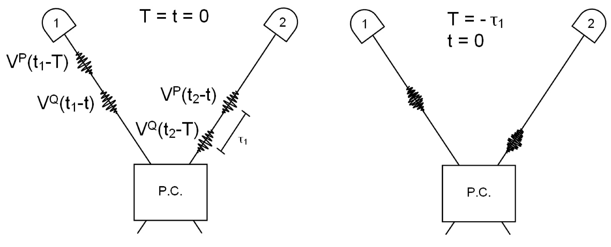
Figure 5: A pictorial representation postponed compensation exchange term photon wave functions in the region of the detectors. The dotted line indicates a two-photon wave function pair and P.C. denotes the postponed compensation apparatus. Once again, in order for interference to occur, all four single-photon amplitudes must overlap. No interference occurs in the separable case, but given a strong enough photon frequency entanglement the exchange terms contribute to the coincidence detection rate. One can observe interference in the frequency entangled case since the spatially displaced exchange term wave functions overlap if $\left|\tau_{1}+(T-t)\right|<\beta$, where $\beta$ is the photon width.

With the finite width assumption Eq. (52) implies $\left|\tau_{1}+(T-t)\right|<\beta$. Fig. 5 is a pictorial representation of how the temporally displaced single-photon wave functions overlap in the region of the detectors to produce non-zero exchange terms given $\left|\tau_{1}+(T-t)\right|<\beta$.

In their discussion of this system, Pittman et al. state that the photons arrive at the beam splitter at much different times. Perhaps there exists some precise definition of what it means for “a photon to arrive at the beam splitter” for which this would be true. However, if one describes the frequency entangled photons according to the wave function picture discussed here, one finds that the wave function amplitudes of both the signal and idler are simultanously non-zero at the beam splitter.

From a broader perspective, of course, we can agree with Pittman et al. that “the intuitively comforting notion of the photons overlapping at the beam splitter is not at the heart of the interference.” One could - although Pittman et al. did not - perform an interference experiment where single-photon amplitudes do not overlap at a particular beam splitter (see Fig. 6). This would demonstrate, as Pittman et al. intended, that the notion of interference arising only when two single photons “meet” at a beam splitter is oversimplistic. Yet such an experiment would not demonstrate any limitation of a description of two-photon interference based on single-photon amplitudes. Even from this broader perspective we feel Pittman et al. go too far when they claim that “two-photon interference cannot be pictured as the interference between two single photons,” at least insofar as it implies that there can be no general model of two-photon interference involving single-photon amplitudes. Indeed, we have presented such a model here. The coincidence detection rate does not explicitly depend on the amplitudes at a particular beam splitter or any other intermediate region, but rather the amplitudes in the detection region. We have shown in Eq. (II) that it is overlapping single-photon amplitudes in the detection region that gives rise to interference.

Strekalov et al.STREKALOV1 claim there are limitations of a single-photon wave packet approach for describing frequency entangled two-photon interference. Using the above theory to describe their experiment, one easily finds that the two-photon interference can in fact be understood in terms of temporally displaced pairs of single-photon amplitudes. In another paper, Kim et al.KIM2 observe quantum interference between two temporally distinguishable pulses and discuss the limitation of a single-photon amplitude description. If one examines their experiment in terms of single-photon wave functions, one can see that the physics is the same as the postponed compensation experiment. The difference between the two experiments is that the temporal distribution is created by a series of pump pulses instead of a CW pump. The 50% visibility observed by Kim et al. is not surprising, at least in the photon wave function picture, as one can see it is simply postponed compensation interference with 50% probability. More recently, Kim and GriceKIM3 report they have observed quantum interference in an experiment where the detected photons retain distinguishing information. Using the photon wavefunction theory to describe their experiment, one finds that the interfering single-photon amplitudes are overlapping in the region of the detectors.

III Conclusion

Using a particular definition of the photon wave function, we have provided the formalism necessary for understanding second-order two-photon intereference in terms of individual photon amplitudes. The theory clarifies the idea of overlapping photons and replaces less rigorous explanations involving distinguishing information or Feynman paths. We have shown that the theory can be applied to both the separable and frequency entangled cases, and that in the latter it allows us to eliminate some of the confusion surrounding the interpretation of two-photon interference. This formalism shows how photon interference can be understood as an exchange effect by drawing an analogy to massive particle wavefunctions.  For the systems discussed here, the presence of exchange terms in the coincidence detection rate expression is a necessary and sufficient condition for second order interference. Furthermore, if one considers only detectors with reasonable detection times and photon pairs with the same center frequency, second order interference is equivalent to the overlap of single photon wave functions in the detection region.

IV Acknowledgements

We would like to thank K.J. Resch, J.S. Lundeen, A.M. Steinberg, and M.G. Raymer for useful discussions. This work was supported by The Natural Sciences and Engineering Research Council of Canada.

Figure 2: A pictorial representation of the Hong-Ou-Mandel exchange term photon wave functions in the region of the detectors. The dotted line indicates a two-photon wave function pair. In order for interference to occur, all four single photon amplitudes must overlap. Photon frequency entanglement allows for interference between temporally displaced two-photon wave functions. However, given that $\delta t$ is larger than the temporal width of the single-photon wave functions there is no interference between temporally displaced wave functions.

Figure 4: A schematic diagram of the postponed compensation experiment. When $\tau_{2}=2\tau_{1}$ interference occurs in the coincidence detection rate despite a delay in mode $b$. Frequency entangled photons are used in this experiment as no interference is observed with a separable photon state as the input.

Figure 6: A schematic diagram of an experiment designed to observe second order interference while the photons do not meet at the central beamsplitter. A separable photon input state is used. With $\tau_{1}=\tau_{2}=\tau_{3}$ maximum interference occurs in the coincidence detection rate.

References

• (1) T.D. Newton and E.P. Wigner, Rev. Mod. Phys. 21, 400 (1949)
• (2) see L. Mandel, Phys. Rev. 144, 1071 (1966); Toshio Inagaki, Phys. Rev. A 57, 2204 (1998) and references therein.
• (3) J.E. Sipe, Phys Rev. A 52, 1875 (1995), Iwo Bialynicki-Birula, “Coherence and Quantum Optics VII” p. 313, Eds. J.H. Eberly, L. Mandel, and E. Wolf. (Plenum, New York, 1996), Margaret Hawton, Phys. Rev. A 59, 3223 (1999)
• (4) K.W. Chan, C.K. Law, and J.H. Eberly, Phys. Rev. Lett. 88, 100402 (2002)
• (5) K.J. Resch, G.G. Lapaire, J.S. Lundeen, J.E. Sipe, and A.M. Steinberg, Phys. Rev. A 69, 063814 (2004)
• (6) L. Mandel and E. Wolf, Optical Coherence and Quantum Optics (Cambridge University Press, New York, 1995).
• (7) H. Fearn and R. Loudon, J. Opt. Soc. Am. B6, 917 (1989).
• (8) C.K. Hong, Z.Y. Ou, and L. Mandel, Phys. Rev. Lett. 59, 2044 (1987)
• (9) Hans-A. Bachor, A Guide to Experiments in Quantum Optics (Wiley-VCH, Weinheim, Germany, 1998)
• (10) M.O. Scully, R. Shea, and J.D. McCullen, Phys. Rep. 43, 485 (1978)
• (11) P.G. Kwiat, A.M. Steinberg, and R.Y. Chiao, Phys. Rev. A 45 7729 (1992); T.J. Herzog, P.G. Kwiat, H. Weinfurter, and A. Zeilinger, Phys. Rev. Lett. 75, 3034 (1995)
• (12) T.B. Pittman, D.V. Strekalov, A. Migdall, M.H. Rubin, A.V. Sergienko, and Y.H. Shih, Phys. Rev. Lett. 77, 1917 (1996)
• (13) R. Graham, T. Wong, M.J. Collett, S.M. Tan, and D.F. Walls, Phys. Rev. A 57 493 (1998)
• (14) Morton H. Rubin, David N. Klyshko, Y.H. Shih, and A.V. Sergienko, Phys. Rev. A 50, 5122 (1994)
• (15) D.V. Strekalov, T.B. Pittman, and Y.H. Shih, Phys. Rev. A 57, 567 (1998)
• (16) Yoon-Ho Kim, Maria V. Checkhova, Sergei P. Kulik, and Yanhua Shih, Phys. Rev. A 60, R37 (1999)
• (17) Yoon-Ho Kim, Warren P. Grice, J. Opt. Soc. Am. B 22, 493 (2005)
Refer to caption