Quantum state engineering in a cavity by Stark chirped rapid adiabatic passage

Abstract

We propose a robust scheme to generate single-photon Fock states and atom-photon and atom-atom entanglement in atom-cavity systems. We also present a scheme for quantum networking between two cavity nodes using an atomic channel. The mechanism is based on Stark-chirped rapid adiabatic passage (SCRAP) and half-SCRAP processes in a microwave cavity. The engineering of these states depends on the design of the adiabatic dynamics through the static and dynamic Stark shifts.

I Introduction

Quantum-state engineering (QSE), i.e., active control over the coherent dynamics of suitable quantum-mechanical systems to achieve a preselected state (e.g. entangled states or multi-photon field states) of the system, has become a fascinating prospect of modern physics. With concepts developed in atomic and molecular physics, the field has been stimulated further by the perspectives of quantum computation and communication.

Single-photon states act as flying qubits in quantum cryptography Jennewein et al. (2000); Naik et al. (2000); Tittel et al. (2000). Key bits can be encoded on the polarization states of single photons; the security of the transmission is based on the fact that a single photon is indivisible and its unknown quantum state cannot be copied. If Alice sends to Bob pulses containing more than one photon, it is possible for a potential evesdropper to measure the photon number in each pulse without disturbing any photons. She can then split off one photon from the pulses that originally contain more than one photon, and retain this photon until Alice and Bob discuss their bases. Such pulses are vulnerable to a photon-number splitting attack. At this point, she can correctly measure the photon polarization and obtain the corresponding bit value without creating any error on Bob’s side. Hence, implementation of quantum cryptography would be secured by a source that emits only one photon at a time. These states can also be used in the error-tolerant quantum computing proposal of Gottesman and Chuang Gottesman and Chuang (1999) which requires that a quantum resource be supplied on demand. Photon fields with fixed photon numbers are also interesting from the point of view of fundamental physics since they represent the ultimate non-classical limit of radiation.

In the context of cavity quantum electrodynamics (CQED), single-photon Fock states have been produced by $\pi$-pulse technique in a microwave cavity Maître et al. (1997); Varcoe et al. (2000) and by the stimulated Raman adiabatic passage (STIRAP) technique in an optical cavity Hennrich et al. (2000) based on the scheme proposed in Parkins et al. (1993) where the Stokes pulse is replaced by a mode of a high-Q cavity. However the $\pi$-pulse technique is not robust with respect to variations of pulse parameters and to exact-resonance condition. The tripod STIRAP process has also been studied in a system of a four-level atom interacting with a cavity mode and two laser pulses, with a coupling scheme which has two globally degenerate dark states Gong et al. (2002). The fractional STIRAP process has also been studied in an optical cavity to prepare atom-photon and atom-atom entanglement Amniat-Talab et al. (2005). Bichromatic adiabatic passage in a microwave cavity is another robust technique that allows one to generate a controlled number of photons in the cavity mode Amniat-Talab et al. (2004). SCRAP is a powerful technique in which the energy of a target state $|+\rangle$ is swept through resonance by a slowly varying dynamic Stark shift to induce complete population transfer from the ground state $|-\rangle$ to the excited state $|+\rangle$. This method uses (i) a laser pulse (the pump) tuned slightly away from the one-photon resonance between the states, and (ii) a relatively intense far-off-resonance pulse (the Stark field) that sweeps the states through the resonance by inducing a dynamic Stark shift. A time delay between the Stark and pump pulses, ensures that the entire population is in the excited state at the end of the process. In this paper we propose a robust scheme in the context of CQED to generate single-photon, atom-photon and atom-atom entangled states based on the SCRAP and the half-SCRAP techniques proposed in the context of laser-driven systems Yatsenko et al. (1999); Yatsenko et al. (2002a).

One can transfer a quantum state by quantum networking. The basic idea behind a quantum network is to transfer a quantum state from one node to another node with the help of a carrier (a quantum channel) such that it arrives intact. In between, one has to perform a process of quantum state transfer (QST) to transfer the state from one node to the carrier and again from the carrier to the destination node. In this paper, using the SCRAP technique in a cavity, we propose a robust scheme for QST to transfer the unknown state of a two-level atom to another atom where the atoms are not directly interacting with each other. We also extend our idea of QST to a quantum network, where we transfer the state of one cavity to another spatially separated cavity. For this we use long-lived atoms as carrier, and make use of the QST process to transfer the state of the cavity to an atom and again to the target cavity.

II construction of the effective Hamiltonian

We consider a two-level atom of upper and lower states $|+\rangle$ and $|-\rangle$ and of energy difference $E_{+}-E_{-}=\omega_{0}$ as represented in Fig. 1. We use atomic units in which $\hbar=1$. The atom initially prepared in its upper state falls through a high-Q microwave cavity with velocity $v$. The atom first encounters the vacuum mode of the cavity with frequency $\omega_{C}$ and waist $W_{C}$ and then the maser beam (Stark field) with frequency $\omega_{S}$ and waist $W_{S}$. The cavity field is near-resonant with the atomic transition, while the Stark field is far-off-resonance that sweeps the states through the resonance by inducing a dynamic Stark shift. The distance between the crossing points of the cavity and the maser axis with the atomic trajectory is $d$. The travelling atom encounters time dependent and delayed Rabi frequency of the cavity mode and the Stark shift:

$$G(t) = G_{0}~{}e^{-(\frac{vt}{W_{C}})^{2}},$$ (1a)

$$S(t) = S_{0}~{}e^{-(\frac{vt\pm d}{W_{S}})^{2}},$$ (1b)

where $S_{0}$ is the peak value of the Stark shift, and $G_{0}=\mu\sqrt{\frac{\omega_{C}}{2\epsilon_{0}V_{\text{mode}}}}$ is the peak value of the cavity’s Rabi frequency with $\mu$, $V_{\text{mode}}$ respectively the dipole moment of the atomic transition, and the effective volume of the cavity mode. In Eq. 1b, the signs $(+,-)$ correspond respectively to paths (a,b) in Fig. 1.

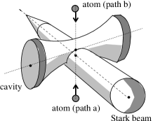
Figure 1: Experimental configuration and linkage pattern of the system. Paths (a) and (b) refer to the paths drawn in Fig. 2.

The detuning of the cavity mode from the atomic transition is $\delta=\omega_{0}-\omega_{C}$. We take the frequency of the cavity field such that $\delta$ is positive and very small with respect to $\omega_{C}$ and $\omega_{0}$. Also we assume

$$\text{max}\{|G(t)|\}\ll\omega_{0},\omega_{C}.$$ (2)

Under these conditions, the counter-rotating terms can be discarded in the rotating-wave approximation (RWA). The semiclassical Hamiltonian of the atom-maser-cavity system can thus be written as

$$H(t) = \omega_{C}a^{{\dagger}}a+\left(\begin{array}[]{cc}\omega_{0}+S_{+}(t)&0\\ 0&S_{-}(t)\\ \end{array}\right)$$ (5)

$$+ G(t)\left(\begin{array}[]{cc}0&a\\ a^{{\dagger}}&0\\ \end{array}\right),$$ (8)

where $a,a^{{\dagger}}$ are the annihilation and creation operators of the cavity mode, and $S_{+,-}(t)$ are the dynamic Stark shifts (proportional to the Stark field intensity) of the bare atomic states. The energy of the lower atomic state has been taken as $0$. This Hamiltonian acts on the Hilbert space $\mathcal{H}\otimes\mathcal{F}$ where $\mathcal{H}$ is the Hilbert space of the atom generated by $|\pm\rangle$ and $\mathcal{F}$ is the Fock space of the cavity mode generated by the orthonormal basis $\{|n\rangle~{};~{}n=0,1,2,\cdots\}$ with $n$ the photon number of the cavity field.

The Hamiltonian $H(t)$ is block-diagonal in the subspaces $\{|+,n\rangle,|-,n+1\rangle;~{}n=0,1,2,...\}$, $|+,n\rangle\equiv|+\rangle\otimes|n\rangle$ and $|n\rangle$ is a $n$-photon Fock state. The vector $|-,0\rangle$ is not coupled to any other ones, i.e., $|-,0\rangle$ is a stationary state of the system. One can thus restrict the problem to the projection of the Hamiltonian in the subspace $\mathcal{S}=\{|+,0\rangle,|-,1\rangle\}$:

$$H_{P} := PHP,$$ (9a)

$$P = |+,0\rangle\left\langle+,0\right|+|-,1\rangle\left\langle-,1\right|,$$ (9b)

if one considers the initial state $|+,0\rangle$. The effective Hamiltonian of the system in the subspace $\mathcal{S}$ can be written as

$$H^{\text{eff}}(t)=\left(\begin{array}[]{cc}\delta+S(t)&G(t)\\ G(t)&0\end{array}\right),$$ (10)

where $S(t)=S_{+}(t)-S_{-}(t)$ is the difference of the Stark shifts of the bare states. The detuning

$$\Delta(t)=\delta+S(t),$$ (11)

is the effective dynamic detuning from one-photon resonance.

We remark that the Stark shifts of the ground and excited states are different. The frequency $\omega_{\text{Stark}}$ of the Stark field should be chosen such that it is not in resonance involving the considered levels. Usually in atoms, one chooses the carrier frequency of the Stark field much smaller than $\omega_{0}$ to prevent e.g. the ionization effects. Under this condition, the coupling of the state $|+\rangle$ to the other atomic upper states (not included in the linkage pattern of Fig. 1) induced by the Stark field, will be larger than their coupling with the state $|-\rangle$ (since it is farther from them) giving $|S_{+}(t)|\gg|S_{-}(t)|$. This results in a reduction of the energy difference between the two states $|-\rangle$ and $|+\rangle$, i.e., $S_{+}(t)<0$.

III Topology of the dressed eigenenergy surfaces

The SCRAP process can be completely described Guérin et al. (2001); Yatsenko et al. (2002b) by the diagram of the two surfaces

$$E_{\pm}(G,\Delta)=\frac{1}{2}(\Delta\pm\sqrt{\Delta^{2}+4G^{2}}),$$ (12)

which represent the eigenenergies as functions of the instantaneous effective Rabi frequency $G$ and Stark shift $S$ (see Fig. 2). All the quantities are normalized with respect to the static detuning $\delta$. The topology of these surfaces, determined by the conical intersections, presents insight into the various adiabatic dynamics which leads to transfer a single photon into the cavity mode by designing appropriate paths connecting the initial and the chosen final state. Each path corresponds to a choice of the envelope of the pulses. In the adiabatic limit, when the pulses vary sufficiently slowly, the solution of the time-dependent Schrödinger equation follows the instantaneous eigenvectors, following the path on the surface that is continuously connected to the initial state. We start with the state $|+,0\rangle$, i.e., the upper atomic state with zero photons in the cavity field. Its energy is shown in Fig. 2 as the starting point of the paths (a), and (b). The paths shown in Fig. 2 describe accurately the dynamics if the time dependence of the envelopes is slow enough according to the Landau-Zener Landau (1932); Zener (1932) and Dykhne-Davis-Pechukas Dykhne (1962); Davis and Pechukas (1976) analysis. If two (uncoupled) eigenvalues cross, the adiabatic theorem of Born and Fock Born and Fock (1928) shows that the dynamics follows diabatically the crossing. This implies that the various dynamics shown in Fig. 2 are a combination of a global adiabatic passage around the conical intersection and local diabatic evolutions through (or in the neighborhood) of conical intersection of the eigenenergy surfaces Guérin et al. (2001).

The eigenenergy surfaces display a conical intersection for $G=0$ and $|S|=\delta$. In the plane $G=0$, the states $|+,0\rangle$ and $|-,1\rangle$ do not interact. Figure 2 shows two possible paths corresponding to SCRAP with $\delta=+|\delta|$ which adiabatically connect the initial state $|+,0\rangle$ to the final state $|-,1\rangle$. For the path (a), while the cavity pulse is off, the Stark pulse is switched on and induces a negative Stark shift $S(t)<0$.

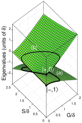
Figure 2: (Color online). Eigenenergy surfaces (in units of $\delta$) of $H^{\text{eff}}$ as functions of the cavity Rabi frequency $G$ and of the Stark shift $S$. The solid paths correspond to adiabatic evolutions which start from $|+,0\rangle$ state and end at $|-,1\rangle$.

Thus, the Stark pulse makes the eigenstates get closer, and induces a resonance with the cavity frequency. This resonance is mute since the cavity pulse is still off, which results in the true crossing in the diagram. The cavity pulse is switched on after the crossing. Later the Stark pulse decreases while the cavity pulse is still on. Finally, the cavity pulse is switched off. The path (b) leads exactly to the same final effect: the cavity pulse is switched on first (making the eigenvalues repel each other as shown in the figure) before the Stark pulse $S(t)$, which is switched off after the cavity pulse.

Inspection of the eigenenergy surfaces in Fig. 2 shows that an essential condition for paths (a),(b) is $S_{0}>\delta$ such that the dynamics goes through the conical intersection (on the $G=0$ plane) between the upper surface (connected to the initial state $|+,0\rangle$) and the lower surface (connected to the final state $|-,1\rangle$). The crossing of this intersection as $S$ varies with $G=0$, brings the system into the lower eigenenergy surface.

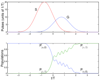
Figure 3: (Color online). Upper panel: the cavity-Stark sequence of Gaussian-shaped pulses [see Eqs. (1a) and (1b)] with the same pulse duration $T$ and pulse parameters $S_{0}=20/T,~{}G_{0}=10/T,~{}\tau=1.5T$, and $\delta=10/T$. Lower panel: the populations of the states $|+,0\rangle$ and $|-,1\rangle$ as functions of time which corresponds to the path (a) in Fig. 2.

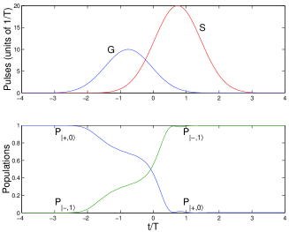
Figure 4: (Color online). Same as Fig. 3, but with the reverse pulse sequence of cavity-Stark which corresponds to the path (b) in Fig. 2. The lower panel shows that the final state of the system will be $|-,1\rangle$ as in Fig. 3.

IV numerical simulation

The dynamics of the system is governed by the Schrödinger equation $i(\partial/\partial t)|\Phi(t)\rangle=H^{\text{eff}}(t)|\Phi(t)\rangle$. The time dependence of parameters of the system are Gaussians of the form (1a), (1b) with the time delay $\tau=d/v$. Figure 3(upper panel) shows the Stark and cavity Gaussian-shaped pulses with the pulse sequence of Stark-cavity and the same pulse duration $T_{C}=W_{C}/v=T=T_{S}=W_{S}/v$ corresponding to the path (a) in Fig. 2. Figure 3(lower panel) presents the time evolution of populations calculated numerically by solving the Schrödinger equation.

Figure 4 represents the reverse pulse sequence of cavity-Stark which corresponds to the path (b) in Fig. 2. We see that for the two sequences of the pulses, the population is completely transferred from the initial state $|+,0\rangle$ to the target state $|-,1\rangle$, i.e., the generation of a single-photon Fock state in the cavity mode with atomic population transfer to the ground state $|-\rangle$ at the end of the SCRAP process.

It can be shown Yatsenko et al. (1999) that for time-delayed Gaussian-shaped pulses (1a) and (1b), the condition of adiabaticity translates to the following requirements for the experimentally controllable pulse parameters $G_{0},~{}T_{C},~{}\delta,~{}S_{0},~{}T_{S},$ and $\tau$,

$$\exp\left(\frac{-8\tau^{2}}{T_{C}^{2}}\right)\ll\frac{\delta}{G_{0}^{2}T_{S}}\sqrt{\ln\frac{S_{0}}{\delta}}\ll 1.$$ (13)

The inequalities (13) imply that it is preferable to work with large cavity-field amplitudes and small static detuning.

The typical value of the cavity lifetime is of the order of $T_{\text{cav}}=1$ ms corresponding to $Q=3\times 10^{8}$, and the upper limit of interaction time is $T_{S}\sim T_{C}\sim T_{\text{int}}=100$ $\mu$s (atom with a velocity of 100 m/s with the cavity mode waist of $W_{C}=6$ mm) Raimond et al. (2001). The condition of global adiabaticity $G_{0}~{}T_{\text{int}}\gg 1$ for the typical value of $G_{0}\approx 0.15$ MHz Raimond et al. (2001) is well satisfied $(G_{0}~{}T_{\text{int}}\approx 15$). Numerics (Figs. 3,4 shows additionally that the diabatic dynamics through the conical intersections of Fig. 2 also satisfied. Closed cavities with higher $Q$ factor $Q=4\times 10^{10}$ and longer decay time $T_{\text{cav}}=0.3$ s may also be used Brattke et al. (2001).

The adiabatic passage can be optimized for a dynamics following a trajectory close to a level line of the difference of the two surfaces of Fig. 2, corresponding to parallel instantaneous eigenenergies Guérin et al. (2002); Guérin and Jauslin (2003).

One issue that needs to be addressed in more detail, is the role of cavity damping which results from the population of the state $|-,1\rangle$ during the time evolution of the system. The cavity damping induce loss that goes from the state $|-,1\rangle$ to the state $|-,0\rangle$, which is not coupled by the effective Hamiltonian. We make the simulation with a loss term in the Schrödinger equation for the state $|-,1\rangle$. This term is $(-i/T_{\text{cav}})$ on the diagonal of the effective Hamiltonian (10) associated to the state $|-,1\rangle$.

Figure 5 (resp. 6) shows that taking into account the cavity damping leads to a final population 0.57 (resp. 0.99) of the state $|-,1\rangle$ for $T_{\text{cav}}=10~{}T_{\text{int}}$ (resp. $T_{\text{cav}}=3000~{}T_{\text{ int}}$), which for $T_{\text{int}}=100~{}\mu$s corresponds to $T_{\text{cav}}=1$ ms (resp. $T_{\text{cav}}=0.3$ s).

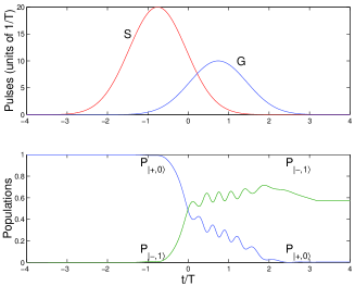
Figure 5: (Color online). Same as Fig. 3, but with inclusion of cavity damping in the effective Hamiltonian as $T_{\text{cav}}=10~{}T_{\text{int}}$. The lower panel shows that the final state of the system will be $|-,1\rangle$ with the population of 0.57.

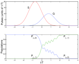
Figure 6: (Color online). Same as Fig. 3, but with inclusion of cavity damping in effective Hamiltonian as $T_{\text{cav}}=3000~{}T_{\text{int}}$. The lower panel shows that the final state of the system will be $|-,1\rangle$ with the population of 0.99.

V atom-photon entanglement

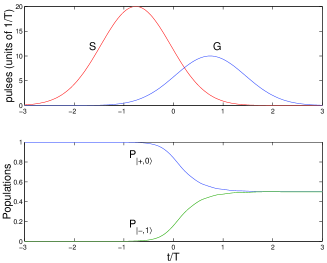
Figure 7: (Color online). Upper panel: Sequence of the Stark and cavity (Gaussian-shaped) pulses with the same parameters of Fig. 3 and $\delta=0$. Lower panel: Populations as function of time which represent a transfer of population from the state $|+,0\rangle$ to a superposition of $|+,0\rangle$ and $|-,1\rangle$ with equal weights (maximally atom-photon entangled state) at the end of the half-SCRAP process.

For a certain range of the cavity detuning $\delta$, the SCRAP technique acts as a fractional SCRAP and will produce a coherent superposition of the states $|+,0\rangle$ and $|-,1\rangle$. The composition of the created superposition is controlled by $\delta$ and is robust against variations in the other interaction parameters. Half SCRAP is a variation of SCRAP for which the cavity detuning $\delta$ is zero, and thus $\Delta=S=-|S|$. Both pulse sequences of cavity-Stark and Stark-cavity leads to the same populations of the states $|+,0\rangle$ and $|-,1\rangle$ at the end of the process. This corresponds to the generation of maximally atom-photon entangled states $\frac{1}{\sqrt{2}}(|+,0\rangle+|-,1\rangle)$. However the sequence of cavity-Stark is not interesting from the view point of applications, since it results in the superposition an additional dynamical phase factor which is difficult to control in a real experiment Yatsenko et al. (2002a). Hence, we consider in the following only the pulse sequence of Stark-cavity.

The instantaneous eigenstates of the effective Hamiltonian (10), or adiabatic states of the system, are as follows:

$$|\phi_{-}\rangle = \cos\vartheta(t)|+,0\rangle-\sin\vartheta(t)|-,1\rangle,$$

$$|\phi_{+}\rangle = \sin\vartheta(t)|+,0\rangle+\cos\vartheta(t)|-,1\rangle,$$ (14)

where the mixing angle $\vartheta(t)$ is defined as

$$\tan 2\vartheta=\frac{G}{\Delta},\qquad 0\leq\vartheta<\pi/2.$$ (15)

When the Stark pulse precedes the cavity pulse, we have:

$$\lim_{t\rightarrow t_{i}}\frac{G}{-|S|}=0,\qquad\lim_{t\rightarrow t_{f}}\frac{G}{-|S|}=-\infty.$$ (16)

This leads to $\vartheta(t_{i})=0$ and $\vartheta(t_{f})=-\pi/4$, and

$$|+,0\rangle\xleftarrow[]{t_{i}\leftarrow t} |\phi_{-}(t)\rangle \xrightarrow[]{t\rightarrow t_{f}}\frac{1}{\sqrt{2}}(|+,0\rangle+|-,1\rangle),$$ (17a)

$$|-,1\rangle\xleftarrow[]{t_{i}\leftarrow t} |\phi_{+}(t)\rangle \xrightarrow[]{t\rightarrow t_{f}}\frac{1}{\sqrt{2}}(-|+,0\rangle+|-,1\rangle).$$ (17b)

Hence if the initial state of the system is taken as $|\Psi(t_{i})\rangle=|+,0\rangle$, the state $|\phi_{-}(t)\rangle$ is the only adiabatic state populated during the whole evolution in the adiabatic limit, and no population will transfer to the other adiabatic state $|\phi_{+}(t)\rangle$. Hence, the system will be driven from the state $|+,0\rangle$ into the superposition

$$|\Psi(t_{f})\rangle=\frac{1}{\sqrt{2}}\left(|+,0\rangle+|-,1\rangle\right),$$ (18)

except for an irrelevant common phase factor.

Figure 7 (upper panel) represents the pulse sequence of Stark-cavity with the same pulse parameters of Fig. 3 and the necessary condition $\delta=0$. We see in the lower panel of this figure that the population is completely transferred from the initial state $|+,0\rangle$ to the target state $\frac{1}{\sqrt{2}}(|+,0\rangle+|-,1\rangle)$, i.e., the generation of a maximally atom-photon entangled state at the end of the half-SCRAP process.

VI atom-atom entanglement

In this section, we show that by combining half-SCRAP and SCRAP processes for two traveling atoms, we can prepare the atoms in a maximally entangled state $\frac{1}{\sqrt{2}}(|+,-\rangle+|-,+\rangle)$. An interesting property of the SCRAP process is that for both of the pulse sequences cavity-Stark and Stark-cavity, the initial states $|+,0\rangle$ and $|-,1\rangle$ evolve as follows:

$$|+,0\rangle\xrightarrow[]{\text{SCRAP}}|-,1\rangle,\qquad|-,1\rangle\xrightarrow[]{\text{SCRAP}}|+,0\rangle.$$ (19)

We also notice that the initial state $|-,0\rangle$ evolves under a SCRAP process as follows:

$$|-,0\rangle\xrightarrow[]{\text{SCRAP}}|-,0\rangle.$$ (20)

In the following we consider the state of the atom1-atom2-cavity system as $|A1,A2,n\rangle$ where $\{A1,A2=+,-\}$, and $\{n=0,1\}$ is the number of photons in the cavity-mode. To create atom-atom maximal entanglement in a microwave cavity, we suppose that the initial state of the combined system is $|+,-,0\rangle$. Two atoms enter successively the cavity mode with different static detunings $\delta$. The first atom encounters the pulse sequence of Stark-cavity in the frame of half-SCRAP process. At the second step, the second atom encounters the same pulse sequence in the frame of SCRAP process. The quantum state of the combined system evolves as follows:

$$|+,-,0\rangle \xrightarrow[]{\text{half-SCRAP}} \frac{1}{\sqrt{2}}(|+,-,0\rangle+|-,-,1\rangle)$$ (21)

$$\xrightarrow[]{\text{SCRAP}} \frac{1}{\sqrt{2}}(|+,-,0\rangle+|-,+,0\rangle),$$

which corresponds to a pair of atoms in a maximally entangled atomic state with an empty cavity. The cavity field which starts and ends up in the vacuum state and remains at the end of the process uncorrelated from the atoms, acts as a catalyst for the atom-atom entanglement.

VII quantum state transfer and quantum networking

In this section we use the SCRAP technique to show that: (i) an unknown state of a two-level atom, $\alpha|-\rangle+\beta|+\rangle$ where $\alpha$ and $\beta$ are unknown arbitrary coefficients, can be transferred to another one with the initial state of $|-\rangle$ through a microwave cavity mode which is initially in the state $|0\rangle$; (ii) an unknown state of a cavity mode $\alpha|0\rangle+\beta|1\rangle$ can be transferred to another cavity (initially in the state $|0\rangle$) through a two-level atom (initially in the state $|-\rangle$).

Figures 8-a,b,c demonstrates how the unknown state $(\alpha|-\rangle+\beta|+\rangle)$ of atom 1 is transferred to atom 2 through the cavity 1 (initially in the state $|0\rangle$). We send the atom 1 through the cavity 1 in the frame of SCRAP process. Equations (19) and (20) shows that the final states of cavity 1 and atom 1 will be $(\alpha|0\rangle+\beta|1\rangle)$, $|-\rangle$ at the end of SCRAP process. After atom 1 comes out of the cavity 1, atom 2 (initially in the state $|-\rangle$) is sent through the cavity 1 (initially in the state $\alpha|0\rangle+\beta|1\rangle$). Atom 2 also experiences a SCRAP process during the interaction with the cavity 1. The final states of cavity 1 and atom 2 at the end of the second SCRAP process will be $|0\rangle$ and $(\alpha|-\rangle+\beta|+\rangle)$ respectively. This means that not only the unknown state $(\alpha|-\rangle+\beta|+\rangle)$ is transferred from atom 1 to atom 2, but also the atoms exchange their states via an interaction with a microwave cavity mode.

Figures 8-b,c,d demonstrates how the unknown state of the cavity 1 is transferred to the cavity 2 (initially in the state $|0\rangle$) by SCRAP technique. We show that we can prepare a quantum network, in which long-lived atomic states (quantum channel) are used to communicate between the two nodes of the network. We assume that there are two identical cavities 1 and 2, which are considered as two nodes of the network. Now our goal is to transfer the state ($\alpha|0\rangle+\beta|1\rangle$) of cavity 1 (node 1) to the cavity 2 (node 2). For that we send an atom (atom 2 in Fig. 8) through the cavity 1. We see that this atom is prepared in the state $(\alpha|-\rangle+\beta|+\rangle)$ at the end of interaction with the node 1. This atom is now sent through the cavity 2 (node 2) which is initially in the state $|0\rangle$. In this way, the unknown state ($\alpha|0\rangle+\beta|1\rangle$) of node 1 is transferred to the node 2. This idea can be extended to a number of distant nodes. For example, to send the state ($\alpha|0\rangle+\beta|1\rangle$) to a third cavity (node 3), we can send a third atom in the same direction after the second one in Fig. 8.

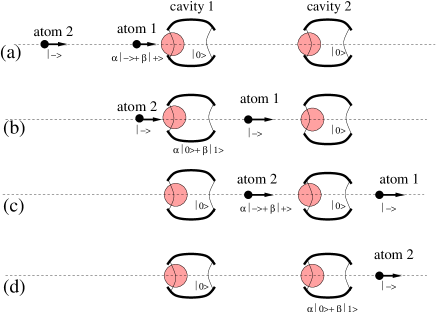
Figure 8: (Color online). Schematic diagram for the QST protocol between two identical atoms via a cavity mode, and for quantum network between two distant cavities via the atomic channel.

VIII discussions and conclusions

Using the topological properties of eigenenergy surfaces of the effective Hamiltonian of the atom-cavity system and SCRAP and half-SCRAP techniques, we have engineered single-photon Fock state and maximally atom-photon and atom-atom entangled states. We also proposed a deterministic way, using SCRAP technique, for quantum networking. This protocol does not require any kind of probability arguments based on the outcome of a measurement. The realization of parameters satisfying the conditions of the proposed schemes appears feasible with progressive improvements to experiments with high-Q microwave cavities. In this analysis we have assumed that the interaction time between the two-state atom and the fields is short compared to the cavity lifetime $T_{\text{cav}}$ and the atom’s excited state lifetime $T_{\text{at}}$, i.e. $T_{\text{int}}\ll T_{\text{cav}},T_{\text{at}}$, which are essential for an experimental setup and avoiding decoherence effects.

The tunable lasers allows the excitation of highly excited atomic states, called Rydberg states. Such excited atoms are very suitable for observing quantum effects in radiation-matter coupling for two reasons: First, these states are very strongly coupled to the radiation field; Furthermore, Rydberg states have relatively long lifetimes with respect to spontaneous decay. In the microwave domain, the radiative lifetime of circular Rydberg states – of the order of $T_{\text{at}}=30$ ms – are much longer than those for non-circular Rydberg states.