Experimental evidence for the breakdown of a Hartree-Fock approach in a weakly interacting Bose gas

Abstract

We investigate the physics underlying the presence of a quasi-condensate in a nearly one dimensional, weakly interacting trapped atomic Bose gas. We show that a Hartree Fock (mean-field) approach fails to predict the existence of the quasi-condensate in the center of the cloud: the quasi-condensate is generated by interaction-induced correlations between atoms and not by a saturation of the excited states. Numerical calculations based on Bogoliubov theory give an estimate of the cross-over density in agreement with experimental results.

Since the first observation of the Bose-Einstein condensation in dilute atomic gases, self consistent mean-field approaches (see e.g. griffinHF ; giorgini97 ) have successfully described most experimental results. A good example is the critical temperature at which the condensate appears shiftTcFabrice ; shiftTcStringari ; Holzmann1999 . However, the approximate treatment made in these theories about particle correlations can not capture all the subtle aspects of the many body problem and the success of these theories relies on the weakness of interactions in dilute atomic gases ($\rho a^{3}\ll 1$ where $\rho$ is the atomic density and $a$ the scattering length for three-dimensional (3D) gases) and also on the absence of large fluctuations (Ginzburg criterion) LandauGinzbourgCriterium . In a 3D Bose gas, this latter criterion is not fulfilled for temperatures very close to the critical temperature shiftTcStringari and deviations from the mean-field theories are expected. For a given atomic density, the critical temperature is calculated to be slightly shifted towards a larger value as compared to the mean-field prediction shiftTcLaloe ; shiftTcMoore ; shiftTcSvistunov but this discrepancy is still beyond the precision of current cold atom experiments shiftTcpiege ; shiftTcFabrice .

In mean-field theory, a Bose gas above condensation is described by a Hartree-Fock (HF) single fluid in which atomic interactions are taken into account only via a mean-field potential $V_{\rm{m.f.}}=2g\rho$lesHouches1999Castin ; StenholmHF where $g$ is the coupling constant and $\rho$ the atomic density. Interaction-induced atomic correlations are neglected and the gas is modeled as a group of non-interacting bosons that experience the self-consistent potential $V_{\rm{m.f.}}$. As for an ideal Bose gas, the two particle correlation function at zero distance $g^{(2)}(0)$ is 2 (bunching effect) LandauGinzbourgCriterium . This HF single fluid description holds until the excited state population saturates, which is the onset of Bose condensation.

In this paper, we present measurements of density profiles of a degenerate Bose gas in a situation where the trap is very elongated and the temperature of the cloud is close to the transverse ground state energy. For sufficiently low temperatures and high densities, we observe the presence of a quasi-condensate Phasefluctu_Petrov at the center of the cloud. Using the above HF theory, we show that a gas with the same temperature and chemical potential as the experimental data is not bose condensed. Thus, a mean-field approach doesn’t account for our results and the quasi-condensate regime is not reached via the usual saturation of the excited states. We emphasize that this failure of mean-field theory happens in a situation where the gas is far from the strong interaction regime, which in one-dimension (1D), corresponds to the Tonks-Girardeau gas limit Kheru2003 ; Bose1D_Lininger ; Phasefluctu_Petrov , and where mean field theory also fails. To our knowledge, this is the first demonstration of the breakdown of a Hartree-Fock approach in the weakly interacting limit.

We attribute this failure of the mean-field theory to the nearly 1D character of the gas. It is well known that a 1D homogeneous ideal Bose gas does not experience Bose Einstein condensation in the thermodynamic limit. On the other hand, in the presence of repulsive interactions in the weakly interacting regime, as the linear density increases one expects a smooth cross-over from an ideal gas regime where $g^{(2)}(0)\simeq 2$ to a quasi-condensate regime where $g^{(2)}(0)\simeq 1$Kheru2003 ; Quasibec_Castin ; Castin1Dclass . The HF approach fails to describe this cross-over: as for an ideal gas, the thermal fluid does not saturate and $g^{(2)}(0)=2$ for any density. The above results also hold for a 1D harmonically trapped gas at the thermodynamic limit: no saturation of excited states occurs for an ideal gas Bagn91 and the gas smoothly enters the quasi-condensate regime when the peak density increasesPhasefluctu_Petrov ; Kheru2005 .

In the experiment presented here, the gas is neither purely 1D nor at the thermodynamic limit: a few transverse modes of the trap are populated and a condensation phenomenon due to finite size effects might be expected Ketterlecond1D . However, we will show that, as in the the scenario discussed above, the gas undergoes a smooth cross-over to the quasi-condensate regime without saturation of the excited states. An estimation of the cross-over density using a three-dimensional Bogoliubov calculation is in agreement with experimental data.

Figure 1: In situ longitudinal distributions for different temperatures (circles). Long dashed lines: ideal Bose gas profile at the shown temperature $T$ and chemical potential $\mu_{0}$ obtained from a fit to the wings. Solid lines: profiles obtained in the Hartree-Fock approximation for the same $T$ and $\mu_{0}$. Short dashed lines: quasi-condensate profiles with the same peak density as the experimental data. Horizontal solid lines: cross-over density estimated using a Bogoliubov calculation (see text).

The experimental setup is the same as esteve2006 . Using a Z-shaped wire on an atom chip Reic99 , we produce an anisotropic trap, with a transverse frequency of $\omega_{\perp}/(2\pi)=2.75$ kHz and a longitudinal frequency of $\omega_{z}/(2\pi)=15.7$ Hz. By evaporative cooling, we obtain a few thousand ⁸⁷Rb atoms in the $|F=2,m_{F}=-2\rangle$ state at a temperature of a few times $\hbar\omega_{\perp}/k_{B}$. Current-flow deformations inside the micro-wire, located 150 $\mu$m below the atoms, produce a roughness on the longitudinal potential Esteve2004 . The observed atomic profiles are smooth (see Fig. 1), which shows that this roughness is small and we neglect it in the following.

The longitudinal profile of the trapped gases are recorded using in situ absorption imaging as in esteve2006 . The probe beam intensity is about 20% of the saturation intensity and the number of atoms contained in a pixel of a CCD camera is deduced from the formula $N_{\rm at}=(\Delta^{2}/\sigma)\rm{ln}({I_{2}}/{I_{1}})$, where $\Delta=6.0~{}\mu$m is the pixel size, $\sigma$ the effective cross section, and $I_{1}$ and $I_{2}$ the probe beam intensity respectively with and without atoms. The longitudinal profiles are obtained by summing the contribution of the pixels in the transverse direction. However, when the optical density is large and the density varies on a scale smaller than the pixel size the above formula underestimates the real atomic density esteve2006 . In our case, the peak optical density at resonance is about $1.5$, and this effect cannot be ignored. To circumvent this problem, we decrease the absorption cross section by detuning the probe laser beam from the $F=2\rightarrow F^{\prime}=3$ transition by $\delta=9$ MHz. We have checked that for larger detunings, the normalised profile remains identical to within 5%. For the detuning $\delta$, the lens effect due to the real part of the atomic refractive index is calculated to be small enough so that all the refracted light is collected by our optical system and the profile is preserved.

To get an absolute measurement of the linear density, we need the effective absorption cross section $\sigma$. We find $\sigma$ by comparing the total absorption of in situ images taken with a detuning $\delta$ with the total number of atoms measured on images taken at resonance after a time of flight long enough (5 ms) that the optical density is much smaller than 1. In these latter images, the probe beam is $\sigma^{+}$ polarized and the magnetic field is pointing along the probe beam propagation direction so that the absorption cross section is $3\lambda^{2}/2\pi$. We obtain for the in situ images taken at a detuning $\delta$, an effective absorption cross section $(0.24\pm 0.04)\times 3\lambda^{2}/2\pi$. For samples as cold as that in Fig. 1 (a), the longitudinal profile is expected to be unaffected by the time of flight and we checked that the profile is in agreement with that obtained from in situ detuned images within 5%.

Averaging over 30 measured profiles, we obtain a relative accuracy of about 5% for the linear density. A systematic error of about 20% is possible due to the uncertainty in the absorption cross section.

In Fig. 1, we plot the longitudinal density profiles of clouds at thermal equilibrium for different final evaporating knives obtained from in situ images. We have compared the density profiles with the expected quasi-condensate density profile with the same peak density. This is obtained using the equation of state of the longitudinally homogeneous gas $\mu=\hbar\omega_{\perp}\sqrt{1+4na}$ Gerbier:771 , and the local chemical potential $\mu(z)=\mu_{0}-1/2m\omega_{z}^{2}z^{2}$, where $n$ is the linear atomic density, and $\mu_{0}$ the chemical potential at the center of the cloud. For the two colder clouds (graphs $(a)$ and $(b)$) in Fig. 1, we observe a good agreement between the central part of the experimental curves (circles) and the quasi-condensate profile (short dashed lines) which indicates that the gas has entered the quasi-condensate regime. In esteve2006 , we observed the inhibition of density fluctuations expected in this regime.

For a given atomic density profile, we extract the temperature and chemical potential of the data from a fit to an ideal Bose gas distribution. For cold clouds, the ideal Bose gas model should fail in the central part of the cloud where interactions are not negligible. We therefore fit only the wings of the profile by excluding a number of pixels $N_{\rm ex}$ on either side of the center of the profile. We fit the longitudinal atomic distribution with only the chemical potential $\mu_{0}$ as a free parameter for different trial temperatures $T$. As seen in Fig. 2, $\mu_{0}(T,N_{\rm ex})$ is approximately linear in $N_{\rm ex}$ for $N_{\rm ex}>10$. The cloud’s temperature is the one for which $\mu_{0}(T,N_{\rm ex})$ is independent of $N_{\rm ex}$. The fluctuations around the straight line for $N_{\rm ex}>10$, seen in Fig. 2, is mainly due to the potential roughness. These fluctuations contribute about for 5% to the uncertainty of $T$ and $\mu_{0}$. The determination of $\mu_{0}$ however, is primarily limited by the uncertainty in the total atom number. For profile (b), we find $T_{b}=(2.75\pm 0.05)\hbar\omega_{\perp}/k_{B}$ and $\mu_{0}^{b}=(1.65\pm 0.5)\hbar\omega_{\perp}$. For the profile (a), the chemical potential and the temperature are not very accurate because the wings are too small. This profile is not analyzed in the following.

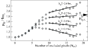
Figure 2: Chemical potential $\mu_{0}$, obtained by fitting the wings of profile (b) to an ideal Bose gas distribution, as a function of the number of excluded pixels $N_{\rm ex}$ on either side of the distribution, for four different trial temperatures. The arrow indicates $\mu_{\rm q.c.}=\hbar\omega_{\perp}\sqrt{1+4n_{0}a}$, which is the chemical potential found from the measured peak linear density $n_{0}$.

Another method to deduce the chemical potential is to use the peak atomic density and the formula $\mu=\hbar\omega_{\perp}\sqrt{1+4na}$, assuming the gas is well inside the quasi-condensate regime at the center of the cloud. For graph $(b)$, we obtain $\mu_{\rm q.c.}^{b}=(1.8\pm 0.2)\ \hbar\omega_{\perp}$, which is consistent with the value obtained from fits of the wings of the distribution.

We now compare the experimental density profiles with the longitudinal atomic density $n(z)$ given by the Hartree Fock theory for the same temperature and chemical potential. To do the calculation, we also assume the relative population of the ground state is negligible (no Bose-Einstein condensation) and the quantization of the longitudinal eigenstates is irrelevant. In this so called local density approximation (LDA), the linear atomic density $n(z)$ is identical to the linear atomic density $n_{h}(\mu(z),T)$ of a thermal Bose gas trapped in the radial direction and longitudinally untrapped at a chemical potential $\mu(z)=\mu_{0}-m\omega_{z}^{2}z^{2}/2$.

To obtain $n_{h}(\mu,T)$, we need to compute the self-consistent three-dimensional atomic density $\rho$ which is the thermodynamic distribution of independent bosons that experience the self consistent HF HamiltonianlesHouches1999Castin ; StenholmHF

$$H_{HF}=\frac{p_{z}^{2}}{2m}+H_{\rm kin}+H_{\rm harm}+2g\rho(r),$$ (1)

where $H_{\rm kin}$ is the transverse kinetic energy term, $H_{\rm harm}$ the transverse harmonic potential, $r$ is the radial coordinate and $g=4\pi\hbar^{2}a/m$ where $a$ is the Rb⁸⁷ scattering length. The simplest approach to obtain $\rho(r)$ is to use an iterative method, starting from $\rho(r)=0$. For each iteration, we numerically diagonalize the transverse part of $H_{HF}$ to deduce the new thermal atomic density distribution. When the interactions become too strong (linear density larger than 320 atoms per pixels for the temperature $T_{b}$) this algorithm does not converge. In this case, we use a more time consuming method based on a minimization algorithm. We use the trial function $\rho_{\rm trial}(r)=\sum c_{2p}H_{2p}(r)e^{-r^{2}/2r_{0}^{2}}$where $H_{2p}(r)$ are Hermite polynomials, and $0\leq\!p\!\leq 3$. We find $r_{0}$ and the four $c_{2p}$ coefficients by minimizing $\xi=\int_{0}^{\infty}r(\rho_{\rm trial}^{{}^{\prime}}(r)-\rho_{\rm trial}(r))^{2}dr/\int_{0}^{\infty}r\rho_{\rm trial}^{2}(r)dr$, where $\rho_{\rm trial}^{{}^{\prime}}(r)$ is the thermodynamic equilibrium atomic density for $H_{HF}[\rho_{\rm trial}(r)]$. We find $\xi$ less than $10^{-4}$ meaning that our 5 parameter model describes the transverse Hartree Fock profile well. The linear density $n_{h}=\int 2\pi r\rho_{\rm trial}(r)dr$ is identical to $n^{\prime}_{h}=\int 2\pi r\rho_{\rm trial}^{\prime}(r)dr$ within $0.5\%$. In the domain where both methods are valid, we also check that they give the same result.

Figure 1 compares the longitudinal profiles obtained with the HF calculation with the experimental data and the ideal gas profile for the graphs $(b),(c)$ and $(d)$. The HF profile for the hottest cloud (graph $(d)$) is in agreement with data and identical within one percent to the ideal Bose gas prediction. For the slightly colder cloud of graph $(c)$, the HF avoids the divergence in the ideal gas model, although it underestimates the peak density by approximately 20%. For the even colder cloud of graph $(b)$, the discrepancy between the HF profile and the experimental data is even larger (35% at the center).

To validate our Hartree Fock calculations we check a posteriori the local density approximation (LDA). The LDA is valid if the population difference between adjacent energy states is negligible. This criterion is met if the absolute value of $\mu_{\rm eff}=\mu_{0}-\varepsilon_{0}(\mu)$ is much larger than $\Delta E$, where $\varepsilon_{0}(\mu)$ is the ground state energy and $\Delta E$ the energy gap between the ground state and the first excited longitudinal state. For the temperature of the graph (b), as long as $\mu_{0}<2.0\hbar\omega_{\perp}$, $|\mu_{\rm eff}/\Delta E|$ is larger than $15$ (see Fig. 3), and for the chemical potential $\mu_{0}^{b}=1.65\hbar\omega_{\perp}$ deduced from the data $|\mu_{\rm eff}/\Delta E|\simeq 25$. For such a large value of $|\mu_{\rm eff}/\Delta E|$, the LDA is expected to be valid.

For this ratio $\mu_{\rm eff}/\Delta E$, we can quantify the error made in the density profile due to the LDA. From the HF calculation, we obtain the energies $E_{n}(\mu,T)$ of the transverse eigenstates. Assuming the transverse motion adiabatically follows the longitudinal one, we obtain an effective longitudinal Hamiltonian with a potential $V_{n}(z)=E_{n}(\mu_{0}-m\omega_{z}^{2}z^{2}/2,T)$ for each transverse mode. Diagonalization of each effective longitudinal Hamiltonian and summation of the resulting thermal profiles gives the expected longitudinal density profile. We find agreement with the profile obtained from the LDA within 5%. This procedure also confirms the LDA for the HF calculations corresponding to the graphs (c) and (d).

In the case of profile $(b)$, where the gas is in the quasi-condensate regime at the center, the Hartree-Fock calculation predicts a population of the ground state $N_{0}\approx k_{B}T/(\varepsilon_{0}-\mu_{0})=0.0035N_{tot}$. Therefore, the Hartree-Fock approach does not predict a saturation of the excited states and fails to explain the presence of the quasi-condensate at the center of the cloud. The local density approximation criterion $|\mu_{\rm eff}|=|\mu_{0}-\varepsilon_{0}(\mu)|>>\Delta E$ also implies a small relative ground state population.

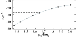
Figure 3: Ratio between the effective chemical potential and $\Delta E$, the energy splitting between the ground state and the first excited state as a function of the chemical potential for the temperature of profile (b). The dashed lines correspond to the measured chemical potential.

The failure of the Hartree-Fock approach for our experimental parameters is due to the large density fluctuations this theory predicts in a dense, nearly 1D gas. When density fluctuations become too large, pair interactions induce correlations in position between particles which are not taken into account in the Hartree-Fock theory. These correlations reduce the interacting energy by decreasing density fluctuations: the gas enters the quasi-condensate regime.

We now estimate the cross-over density $n_{\rm c.o.}$ at which the gas enters the quasi-condensate regime. For this purpose, we assume the gas is in the quasi-condensate regime and use the Bogoliubov theory to compute density fluctuations. We find a posteriori the validity domain of the quasi-condensate regime, which requires that density fluctuations $\delta\rho$ be small compared to the mean density $\rho$. More precisely, we define $n_{\rm c.o.}$ as the density for which the Bogoliubov calculation yields $\int\!\!\int(\delta\rho(r))^{2}\!/\!(\rho(r)n_{\rm c.o.})\ d^{2}r=1$. We indicate this cross-over density in Fig.1. We find that $n_{\rm c.o.}$ is close to the density above which the experimental profiles agree with the quasi-condensate profile.

In conclusion, we have been able to reach a situation where a quasi-condensate is experimentally observed but a HF approach fails to explain its presence. As for purely one dimensional systems, the passage towards quasi-condensate in our experiment is a smooth cross-over driven by interactions. The profiles that we observe require a more involved theory able to interpolate between the classical and the quasi-condensate regime. A Quantum Monte Carlo calculation that gives the exact solution of the many body problem shiftTcSvistunov ; Holzmann1999 should reproduce the experimental data. In fact, since temperatures are larger than interaction energy, quantum fluctuations of long wavelength excitations should be negligible and a simpler classical field calculation should be sufficient Goral2002 ; Davis2006 . Finally, the refined mean field theory proposed in StoofHFmod , where the coupling constant $g$ is modified to take into account correlations between atoms, may explain our profiles.

We thank A. Aspect and L. Sanchez-Palencia for careful reading of the manuscript, and D. Mailly from the LPN (Marcoussis, France) for help in micro-fabrication. The atom optics group is member of l’Institut Francilien de la Recherche sur les Atomes Froids. This work has been supported by the EU under grants MRTN-CT-2003-505032, IP-CT-015714.

References

- (1) A. Griffin, Phys. Rev. B 53, 9341 (1996).
- (2) S. Giorgini, L. P. Pitaevskii, and S. Stringari, J. Low Temp. Phys. 109, 309 (1997).
- (3) F. Gerbier et al., Phys. Rev. Lett. 92, 030405 (2004).
- (4) S. Giorgini, L. P. Pitaevskii, and S. Stringari, Phys. Rev. A 54, R4633 (1996).
- (5) M. Holzmann, W. Krauth, and M. Naraschewski, Phys. Rev. A 59, 002956 (1999).
- (6) Y. Castin in “Coherent atomic matter waves” (Springer,Berlin) 2001, R. Kaiser, C. Westbrook, F.David,Eds. p32-36
- (7) P. Öhberg and S. Stenholm, J. Phys. B 30, 2749 (1997)
- (8) L. Landau and E. Lifschitz, in Statistical physics, Part I (Pergamon, Oxford, 1980), Chap. 14.
- (9) M. Holzmann, G. Baym, J.-P. Blaizot, and F. Laloë, Phys. Rev. Lett. 87, 120403 (2001).
- (10) P. Arnold and G. Moore, Phys. Rev. Lett. 87, 120401 (2001).
- (11) V. A. Kashurnikov, N. V. Prokofév, and B. V. Svistunov, Phys. Rev. Lett. 87, 120402 (2001).
- (12) P. Arnold and B. Tomàŝik, Phys. Rev. A 64, 053609 (2001).
- (13) K. V. Kheruntsyan, D. M. Gangardt, P. D. Drummond, and G. V. Shlyapnikov, Phys. Rev. Lett. 91, 040403 (2003).
- (14) E. H. Lieb and W. Liniger, Phys. Review 130, 1605 (1963).
- (15) D. Petrov, G. Shlyapnikov, and J. Walraven, Phys. Rev. Lett. 85, 3745 (2000).
- (16) C. Mora and Y. Castin, Phys. Rev. A 67, 053615 (2003).
- (17) Y. Castin et al., J. Modern Opt. 47, 2671 (2000).
- (18) V. Bagnato and D. Kleppner, Phys. Rev. A 44, 7439 (1991).
- (19) K. V. Kheruntsyan, D. M. Gangardt, P. D. Drummond, and G. V. Shlyapnikov, Phys. Rev. A 71, 053615 (2005) .
- (20) W. Ketterle and N. J. van Druten, Phys. Rev. A 54, 656 (1996).
- (21) J. Est ve et al., Phys. Rev. Lett. 96, 130403 (2006).
- (22) J. Reichel, W. Hänsel, and T. W. Hänsch, Phys. Rev. Lett. 83, 3398 (1999).
- (23) J. Esteve et al., Phys. Rev. A 70, 043629 (2004).
- (24) F. Gerbier, Europhys. Lett. 66, 771 (2004).
- (25) K. Góral, M. Gadja, and K. Rza̧ızewski, Phys. Rev. A 66, 051602 (2002).
- (26) M. J. Davis and P. B. Blakie, Phys. Rev. Lett. 96, 060404 (2006).
- (27) Al Khawaja et al., Phys. Rev. A 66, 13615 (2002)