Non-Hermitian degeneracy of two unbound states

Abstract

We solved numerically the implicit, trascendental equation that defines the eigenenergy surface of a degenerating isolated doublet of unbound states in the simple but illustrative case of the scattering of a beam of particles by a double barrier potential. Unfolding the degeneracy point with the help of a contact equivalent approximant, crossings and anticrossings of energies and widths, as well as the changes of identity of the poles of the $S-$matrix are explained in terms of sections of the eigenenergy surfaces.

1 Introduction

Unbound decaying states are energy eigenstates of a time reversal invariant Hamiltonian describing non-dissipative physics in a situation in which there are no particles incident [1, 2]. Even when the formal Hamiltonian, considered as an operator in the Hilbert space of square integrable functions, is Hermitian (self-adjoint), this boundary condition makes the eigenvalue problem non-selfadjoint and the corresponding energy eigenvalues complex, ${\cal E}_{n}=E_{n}-i1/2\Gamma_{n}$ with $E_{n}>\Gamma_{n}>0$ [3].

Commonly, unbound energy eigenstates are regarded as arising from a perturbation with the physics essentially unchanged from the bound state case, except for an exponential decay. But, unbound state physics differs radically from bound state physics in the presence of degeneracies that is, coalescence of eigenvalues [4].

In the case of a Hermitian Hamiltonian depending on parameters, the bound state energy eigenvalues are real and, when a single parameter is varied, the mixing of two levels leads to the well known phenomenon of energy level repulsion [5] and avoided level crossing [6]. In the case of unbound energy eigenstates (resonances) of the same Hamiltonian, the energy eigenvalues are complex and, when a single parameter is varied, this fact opens a rich variety of possibilities, namely, crossings and anticrossings of energies and widths [7], and the so called “change of identity” of the poles of the $S-$matrix [8]. These novel effects have attracted considerable theoretical [9, 10, 11] and recently also experimental interest [12]. True degeneracies of resonance energy eigenvalues result from a joint crossing of energies and widths in a physical system depending on only two real parameters and give rise to the occurrence of a double pole of the scattering matrix in the complex energy plane [10]. Associated with a double pole of the $S-$matrix, the quantum system has a chain of Jordan-Gamow generalized eigenfunctions [3, 13, 14]. Examples of double poles in the scattering matrix of simple quantum systems have been recently described [15, 16, 17, 18]. Degeneracy of complex energy eigenvalues of non-Hermitian PT symmetric Hamiltonian has been discussed by M. Znojil [19, 20, 21] and A. Mostafazadeh [22]. From a phenomenological point of view, I. Rotter discussed double poles in the scattering matrix and level repulsion of unbound states in the framework of an effective many body theory [23, 24, 25, 26] .

The characterization of the singularities of the eigenenergy surfaces at a degeneracy of unbound states in parameter space arises naturally in connection with the Berry phase of unbound states that was predicted by Hernández et al [27, 28, 29] and independently by W.D. Heiss [30], see also the interesting recent work by A.A. Mailybaev et al [31]. The Berry phase of two unbound states was measured by the Darmstadt group [32, 33]. The unfolding of energy eigenvalue surfaces at a degeneracy of unbound states of a Hermitian Hamiltonian was discussed by E. Hernández et al [34] and the unfolding of eigenvalue surfaces of non-Hermitian Hamiltonian matrices with applications in modern problems of quantum physics, cristal optics, physical chemistry, acoustics, mechanics and circuit theory has been the subject of many recent investigacions [35, 36, 37, 38, 39, 40, 41, 42].

In this paper, we will be concerned with some physical and mathematical aspects of the mixing and degeneracy of two unbound energy eigenstates in an isolated doublet of resonances of a quantum system depending on two control parameters. The plan of the paper is as follows: In section 2, we give the results of a numerical computation of the surfaces that represent the resonance energy eigenvalues as functions of the control parameters in the scattering of a beam of particles by a double barrier potential. The analytical structure of the singularity of the energy surface at the crossing point is characterized in section 3, where we also introduce a contact equivalent approximant to the energy surface at the degeneracy point. Section 4 is devoted to a discussion of crossings and anticrossings of energies and widths, as well as, the changes of identity of the poles of the $S-$matrix, in term of sections of the energy surfaces. We end our paper with a short summary and some conclusions.

2 Resonances in a double barrier potential

Doublets of resonances and accidental degeneracies of unbound states may occur in the scattering of a beam of particles by a potential with two regions of trapping. A simple example is provided by a spherically symmetric potential $V(r)$ such that the two regions of trapping are two potential wells defined by two concentric potential barriers located between the origin of coordinates and the outer region where the potential $V(r)$ vanishes. In order to make the analysis as simple and explicit as possible, we take the wells and barriers to be square as shown in figure 1.

Figure 1: The double barrier potential is such that it supports two unbound states with equal energies and half-lives. The control parameters of the system are $d$ and $V_{3}$.

In this section, we will consider the conditions for the occurrence of a degeneracy of unbound states in this simple system and we will describe the numerically exact computation of the surfaces that represent the complex energy eigenvalues as functions of the control parameters of the system in the neighbourhood of and at a degeneracy of unbound states.

2.1 The Jost regular solution

The s-wave radial Schrödinger equation is

$$\frac{d^{2}\phi(k,r)}{dr^{2}}+(k^{2}-U(r))\phi(k,r)=0,$$ (1)

the potential $U(r)=2mV(r)/\hbar^{2}$ is a double barrier such that between the origin of coordinates and the outer region, where the particles propagate freely, there are two square potential wells separated by two square potential barriers, as shown in figure 1. The system has seven parameters, the positions $r_{i}$ (i = 1,2,3,4) and heights $V_{i}$ (i = 2,3,4) of the four discontinuities of the potential. We will keep the five parameters $(V_{2},V_{4},r_{1},r_{3}-r_{2},r_{4}-r_{3})$ fixed and will vary the depth $V_{3}$ of the outer well and the thickness of the inner barrier $d=r_{2}-r_{1}$. In the following, we will refer to the pair of parameters $(d,V_{3})$ as the control parameters of the system.

The radial Schrödinger equation (1) is solved exactly. The Jost regular solution of (1) normalized to unit slope at the origen, $\phi(k,r)$, is as follows:

In the wells,

$$\phi_{1}(k,r)=\frac{1}{k}\sin kr,\hskip 42.67912pt0\leq r\leq r_{1},$$ (2)

and

$$\phi_{3}(k,r) = \phi_{2}(k,r_{2})\Bigl{[}\cos\Bigl{(}K_{3}(k,V_{3})(r-r_{2})\Bigr{)}$$ (3)

$$+ \alpha_{2}(k,d)\sin\Bigl{(}K_{3}(k,V_{3})(r-r_{2})\Bigr{)}\Bigr{]},\hskip 8.5359ptr_{2}\leq r\leq r_{3}.$$

In the barriers,

$$\phi_{i}(k,r) = \phi_{i-1}(k,r_{i-1})\Bigl{[}\cosh\Bigl{(}K_{i}(k)(r-r_{i-1})\Bigr{)}$$

$$+ \alpha_{i-1}(k,d)\sinh\Bigl{(}K_{i}(k)(r-r_{i-1})\Bigr{)}\Bigr{]},\hskip 14.22636ptr_{i-1}\leq r\leq r_{i},\ \ \ i=2,4,$$

and, in the outer region,

$$\phi_{5}(k,r)=\phi_{4}(k,r_{4})\Bigl{[}\cos k(r-r_{4})+\alpha_{4}(k,d)\sin k(r-r_{4})\Bigr{]},\ \ \ r_{4}\leq r<\infty.$$

In these expressions $k$ is the wave number of the free waves and

$$K_{i}(k)=\Bigl{(}(-1)^{i}(U_{i}-k^{2})\Bigr{)}^{1/2},\hskip 28.45274pti=2,3,4$$ (6)

is the wave number in the barriers and the outer well.

The logaritmic derivatives $\alpha_{i}(k,d,V_{3})$ of $\phi(k,r)$ at the consecutive discontinuities $r_{i}$ and $r_{i+1}$ are related by the matching conditions at $r_{i+1}$,

$$\alpha_{1}(k)=\frac{k}{K_{2}(k)}\cot kr_{1},\hskip 19.91684pt\alpha_{2}(k,d)=\frac{K_{2}(k)}{K_{3}(k)}\frac{\alpha_{1}(k)+\tanh(K_{2}(k)d)}{1+\alpha_{1}(k)\tanh(K_{2}(k)d)},$$ (7)

$$\alpha_{3}(k;d,V_{3})=\frac{K_{3}(k,V_{3})}{K_{4}(k)}\frac{\alpha_{2}(k,d)-\tan(K_{3}(k)(r_{3}-r_{2}))}{1+\alpha_{2}(k,d)\tan(K_{3}(k)(r_{3}-r_{2}))},$$ (8)

and

$$\alpha_{4}(k;d,V_{3})=\frac{K_{4}(k)}{k}\frac{\alpha_{3}(k;d,V_{3})+\tanh(K_{4}(k)(r_{4}-r_{3}))}{1+\alpha_{3}(k;d,V_{3})\tanh(K_{4}(k)(r_{4}-r_{3}))}.$$ (9)

Since the first logaritmic derivative is known, succesive substitution of $\alpha_{i}(k,d,V_{3})$ in $\alpha_{i+1}(k,d,V_{3})$ gives an explicit solution for $\alpha_{4}(k;d,V_{3})$ and an explicit expression for the regular solution is obtained from equations (2-2.1).

2.2 The Jost function

When the regular solution in the outer region, (2.1), is written as a linear combination of an outgoing wave $\exp(ikr)$ and an incoming wave $\exp{(-ikr)}$

$$\phi_{5}(k,r) = \phi_{4}(k,r_{4})\frac{1}{2}\Bigl{[}\Bigl{(}1-i\alpha_{4}(k;V_{3},d)\Bigr{)}\exp{ik(r-r_{4})}$$ (10)

$$+ \Bigl{(}1+i\alpha_{4}(k;V_{3},d)\Bigr{)}\exp{-ik(r-r_{4})}\Bigr{]},\hskip 28.45274ptr_{4}\leq r<\infty,$$ (11)

the coefficient of the incoming wave is the Jost function. Making use of equations (2.1), (9) and (10) we find an exact expression for the Jost function $f(-k)$,

$$f(-k;d,V_{3})=\sin kr_{1}\Bigl{[}\cosh K_{2}(k)d+\alpha_{1}(k)\sinh K_{2}(k)d\Bigr{]}$$

$$\times\Bigl{[}\cos K_{3}(k,V_{3})(r_{3}-r_{2})+\alpha_{2}(k,d,V_{3})\sin K_{3}(k,V_{3})(r_{3}-r_{2})\Bigr{]}$$

$$\times\Bigl{\{}\frac{K_{4}(k)}{k}\Bigl{[}\sinh K_{4}(k)(r_{4}-r_{3})+\alpha_{3}(k;d,V_{3})\cosh K_{4}(k)(r_{4}-r_{3})\Bigr{]}$$

$$-i\Bigl{[}\cosh K_{4}(k)(r_{4}-r_{3})+\alpha_{3}(k;d,V_{3})\sinh K_{4}(k)(r_{4}-r_{3})\Bigr{]}\Bigr{\}}\exp ikr_{4}$$ (12)

2.3 The physical solutions

The scattering wave function, $\psi(k,r)$, and the regular solution $\phi(k,r)$ are related by [43]

$$\psi(k,r)=\frac{-2ik}{f(-k)}\phi(k,r),$$ (13)

and the scattering matrix is given by

$$S(k)=\frac{f^{*}(-k)}{f(-k)}=\exp(i2\delta(k)),$$ (14)

where the Jost function $f(-k)$ is given by (2.2).

The zeros of the Jost function give resonance poles in the scattering wave function $\psi(k,r)$, and in the $S(k)$ matrix, and from (1) and (2-2.1), we may verify that all unbound energy eigenfunctions of the radial Schrödinger equation are associated with roots (zeros) of the Jost function.

Unbound state eigenfunctions also called resonant-state or Gamow eigenfunctions are the solutions of equation (1) that vanish at the origin, and at infinity satisfy the outgoing wave boundary condition. When the Jost function has a zero at $k_{n}$, the coefficient of the incoming wave in (10) vanishes, and $\phi(k_{n},r)$ is proportional to the outgoing wave solution of equation (1) for $r$ larger than the range of the potential. Hence, the unbound state eigenfunctions are related to the regular solution by

$$u_{n}(k_{n},r)=N^{-1}_{n}\phi(k_{n},r),$$ (15)

where $N_{n}$ is a normalization constant and $k_{n}$ is a zero of the Jost function

$$f(-k_{n};d,V_{3})=0$$ (16)

2.4 Degeneracy of unbound energy eigenvalues

A degeneracy of unbound states results from the exact coincidence of two simple zeros of the Jost function, which merge into one double zero lying in the fourth quadrant of the complex $k-$plane. Hence, the condition for a degeneracy of two unbound energy eigenstates at some $k=k_{d}$ is that both, the Jost function and its first derivative vanish at $k_{d}$,

$$f(-k_{d};d,V_{3})=0,\hskip 36.98866pt\Bigl{(}\frac{df(-k;d,V_{3})}{dk}\Bigr{)}_{k_{d}}=0,$$ (17)

where $f(-k;d,V_{3})$ is given in (2.2).

Therefore, to locate a degeneracy of unbound states, the coupled equations (17) were solved numerically. The zeroes of the Jost function are found by an algebraic computer package that searches for the minima of $|f(-k)|$ in the complex k-plane. In the computation the five parameters $V_{2},V_{4},r_{1},r_{3}-r_{2}$ and $r_{4}-r_{3}$ were kept fixed at the values $V_{2}=V_{4}=2,r_{1}=1,r_{3}-r_{2}=1,r_{4}-r_{3}=$ 0.304892 and only the control parameters $d$ and $V_{3}$ were allowed to vary. Starting with the values $d=$ 2 and $V_{3}=$ 1.04, we find the first isolated doublet of resonances at $k_{1}=$ 2.2101546 - i 0.1366887 and $k_{2}=$ 2.2321776 - i 0.0017984.

Then, we adjusted the control parameters $d$ and $V_{3}$ until $k_{1}$ and $k_{2}$ became equal to some common value $k_{d}$. We also computed numerically $|df(-k)/dk|$ at $k=k_{d}$ to verify that the second equation was also satisfied to some previously prescribed accuracy. In this way, we found that by fine tuning the control parameters to the values $d^{*}=1.1314661145$ and $V_{3}^{*}=1.038235081$, the first doublet of resonances becomes degenerate, with a precision better than one part in $10^{8}$, at $k_{d}=$ 2.22697606 - i 0.07220139.

In the following we will refer to the double zero of $f(-k)$ at $k_{d}$ as the degeneracy point or crossing point of the doublet of resonant states in the complex k-plane and to the point $(d^{*},V^{*}_{3})$ as the exceptional point in parameter space.

2.5 Energy surfaces

The energy eigenvalues ${\cal E}_{n}(d,V_{3})=(\hbar^{2}/2m)k^{2}_{n}(d,V_{3})$ of the physical system are obtained from the zeroes of the Jost function, given in equation (16). That condition defines, implicitly, the inverse functions

$$k_{n}(d,V_{3})=f^{-1}(0;d,V_{3}),\hskip 28.45274ptn=1,2,....$$ (18)

as branches of a multivalued function [43] which will be called the wave number pole position function. Each branch $k_{n}(d,V_{3})$ is a continuous, single valued function of the control parameters. When the physical system has an isolated doublet of unbound states which become degenerate for some exceptional values of the control parameters $(d^{*},V_{3}^{*})$, the corresponding two branches of the energy pole position function, ${\cal E}_{1}(d,V_{3})$ and ${\cal E}_{2}(d,V_{3})$, are equal (cross or coincide) at that point.

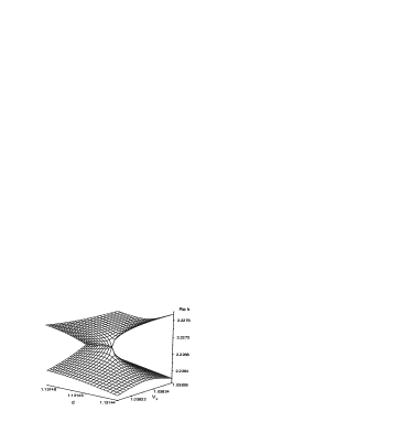
Figure 2: The two - sheeted surface $S_{R}$ that represents the real part of the eigenwave numbers $k_{1}$ and $k_{2}$ as functions of the control parameters $(d,V_{3})$ in the vecinity of a degeneracy of unbound states.

With the purpose of exploring the geometrical and topological properties of the surfaces representing the pole position function $k_{1,2}(d,V_{3})$ of the isolated doublet of resonances in parameter space, we solved numerically the implicit equation (16) for $k_{1}(d,V_{3})$ and $k_{2}(d,V_{3})$ in the neighbourhood of and at a degeneracy of unbound states. The results of the numerical computation are represented as surfaces in a Euclidean space with coordinates (Re $k$, Im $k$, d, $V_{3}$).

In figure 2, the real function Re $k_{1,2}(d,V_{3})$ is shown as a surface $S_{R}$ in the three-dimensional subspace with cartesian coordinates (Re $k,d,V_{3}$). Similarly, in figure 3, the real function Im $k_{1,2}(d,V_{3})$ is shown as a surface $S_{I}$ in the three-dimensional subspace with cartesian coordinates (Im $k,d,V_{3}$).

We see that close to the degeneracy of unbound states, the function Re $k_{1,2}(d,V_{3}$) has two branches and is represented by a two sheeted surface $S_{R}$. The two sheets of $S_{R}$ are two copies of the plane $(d,V_{3})$ which are cut and joined smoothly along a line ${\cal L}_{R}$ starting at the exceptional point and extending to values $d\geq d^{*}$ and $V_{3}\geq V^{*}_{3}$.

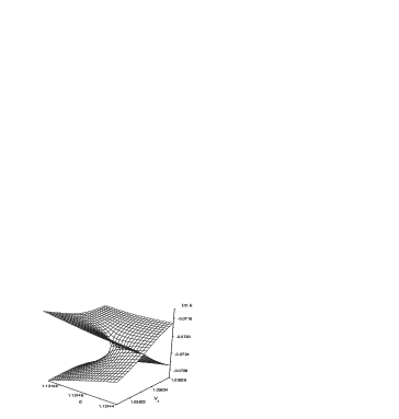
Figure 3: The two-sheeted surface $S_{I}$ that represents the imaginary part of eigenwave numbers $k_{1}$ and $k_{2}$ as functions of the control parameters $(d,V_{3})$ in the neighbourhood of a degeneracy of unbound states with complex resonance energies ${\cal E}_{i}=\hbar^{2}k^{2}_{i}/2m$, $i=1,2$.

The function Im $k_{1,2}(d,V_{3})$ has also two branches and is represented by a two sheeted surface $S_{I}$. The two sheets of $S_{I}$ are two copies of the plane $(d,V_{3})$ which are cut and pasted smoothly along a line ${\cal L}_{I}$ extending from the exceptional point to values $d\leq d^{*}$ and $V_{3}\leq V^{*}_{3}$.

The projection of the lines ${\cal L}_{R}$ and ${\cal L}_{I}$ on the plane $(d,V_{3})$ are the two halves of a line ${\cal L}^{\prime}$ that goes through the exceptional point $(d^{*},V^{*}_{3})$.

At the exceptional point, and only at that point, both the real and imaginary parts of $k_{1}$ and $k_{2}$ are equal. Therefore, in the complex k-plane, at the crossing point, the two simple zeroes of the Jost function merge into one double zero which is an isolated point in the complex k-plane.

3 The analytical behaviour of the pole-position function close to the exceptional point

In this section, it will be shown that, the singularity of the energy surface at the degeneracy or crossing point is an algebraic branch point of square root type. The analytical structure of the singularity of the energy surface will be worked out and discussed in detail. The results in this and the following section are not restricted to the double barrier potential, to stress this generality, the control parameters will be called $x_{1}$ and $x_{2}$.

Let us start by recalling that, when the first and second absolute moments of the potential exist, and the potential decreases at infinity faster than any exponential [e.g., if $V(r)$ has a Gaussian tail or if it vanishes identically beyond a finite radius], the Jost function $f(-k;x_{1},x_{2})$, is an entire function of $k$ [43]. The entire function of $k$, $f(-k;x_{1},x_{2})$, may be written in the form of an infinite product, according to Hadamard’s form of the Weierstrass factorization theorem [44], and by using a theorem of Pfluger [45], we may write

$$f(-k;x_{1},x_{2})=f(0)\exp({ikR})\prod_{1}^{\infty}\Bigl{(}1-\frac{k}{k_{n}(x_{1},x_{2})}\Bigr{)}$$ (19)

$R$ is the range of the potential, $f(0)\neq 0$ and $\{k_{n}\}$ are the zeroes of $f(-k;x_{1},x_{2})$, see also R.G. Newton [43].

When the Jost function has a set of isolated zeroes, the implicit equation for the pole position function, equation (16), may, in principle, be solved, at least numerically, for each branch $k_{n}(x_{1},x_{2})$ without ambiguity. When the system has an isolated doublet of resonances which may become degenerate, the corresponding branches of the pole position function, say $k_{1}(x_{1},x_{2})$ and $k_{2}(x_{1},x_{2})$, may be equal (cross or coincide) at an exceptional point. In this case, it is not possible to solve equation (16) for each individual branch without ambiguity and one should proceed to solve that equation for the pole position function of the two members of the isolated doublet of resonances.

To be precise, we will say that the system has an isolated doublet of unbound states if there is a finite bounded and connected region ${\cal M}$ in parameter space and a finite domain ${\cal D}$ in the fourth quadrant of the complex $k-$plane, such that when $(x_{1},x_{2})\ \epsilon\ {\cal M}$, the Jost function has two and only two zeroes, $k_{1}$ and $k_{2}$, in the finite domain ${\cal D}\subset{\cal C}$, all other zeroes of $f(-k;x_{1},x_{2})$ lying outside ${\cal D}$.

The pole position function $k_{1,2}(x_{1},x_{2})$ of the isolated doublet of resonances,

$$k_{1,2}(x_{1},x_{2})=f^{-1}(0;x_{1},x_{2}),$$ (20)

is implicitly defined by the equation $f(-k_{1,2};x_{1},x_{2})=0$, and the conditions

$$\Bigl{(}\frac{df(-k;x_{1},x_{2})}{dk}\Bigr{)}_{k_{d}}=0,\hskip 28.45274pt\mbox{and}\hskip 28.45274pt\Bigl{(}\frac{d^{2}f(-k;x_{1},x_{2})}{dk^{2}}\Bigr{)}_{k_{d}}\neq 0,$$ (21)

for $(x_{1},x_{2})$ in a neighbourhood of the exceptional point $(x_{1}^{*},x_{2}^{*})$.

Then, to find an expression for the pole position function of the isolated doublet of unbound states, the two zeroes of $f(-k;x_{1},x_{2})$, corresponding to the isolated doublet of unbound states are explicitly factorized in (19) as

$$f(-k;x_{1},x_{2})=\Bigl{[}k-k_{1}(x_{1},x_{2})\Bigr{]}\Bigl{[}k-k_{2}(x_{1},x_{2})\Bigr{]}g_{1,2}(k;x_{1},x_{2}),$$ (22)

which may be conveniently rearranged as

$$\begin{array}[]{c}f(-k;x_{1},x_{2})=\Bigl{[}\bigl{(}k-\frac{1}{2}(k_{1}+k_{2})\bigr{)}^{2}-\frac{1}{4}\bigl{(}k_{1}-k_{2}\bigr{)}^{2}\Bigr{]}g_{1,2}(k,x_{1},x_{2}).\end{array}$$ (23)

with

$$g_{1,2}(k;x_{1},x_{2})=f(0)\exp(ikR)\frac{1}{k_{1}(x_{1},x_{2})k_{2}(x_{1},x_{2})}\prod_{3}^{\infty}\Bigl{(}1-\frac{k}{k_{n}(x_{1},x_{2})}\Bigr{)},$$ (24)

the expression in square brackets in the right hand side of equation (23) is the Weierstrass polynomial of the isolated doublet of unbound states[46].

Solving equation (23) for $k_{1,2}(x_{1},x_{2})$ when $f(-k;x_{1},x_{2})$ vanishes, we get

$$k_{1,2}(x_{1},x_{2})=\frac{1}{2}\Big{(}k_{1}(x_{1},x_{2})+k_{2}(x_{1},x_{2})\Bigr{)}+\sqrt{\frac{1}{4}\Big{(}k_{1}(x_{1},x_{2}\bigr{)}-k_{2}\bigl{(}x_{1},x_{2}\bigr{)}\Bigr{)}^{2}}$$ (26)

with $(x_{1},x_{2})$ in a neighbourhood of the exceptional point. This equation relates the wave number pole position function of the doublet to the pole position function of the individual unbound (resonance) states. Since the argument of the square-root function is complex, it is necessary to specify the branch. Here and thereafter, the square root of any complex quantity $F$ will be defined by

$$\sqrt{F}=|\sqrt{F}|\exp\bigl{(}i\frac{1}{2}argF\bigr{)},\hskip 28.45274pt0\leq arg\ F\leq 2\pi$$ (28)

so that $|\sqrt{F}|=\sqrt{|F|}$ and the $F-$ plane is cut along the real axis.

Now, we will proceed to the derivation of a contact equivalent approximant to the pole position function of the doublet at the crossing point.

According to the preparation theorem of Weierstrass [46], the functions $1/2(k_{1}(x_{1},x_{2})+k_{2}(x_{1},x_{2}))$ and $1/4(k_{1}(x_{1},x_{2})-k_{2}(x_{1},x_{2}))^{2}$, appearing in the right hand side of equation (26), are regular at the exceptional point and admit a Taylor series expansion about that point,

$$\frac{1}{2}\Bigl{(}k_{1}(x_{1},x_{2})+k_{2}(x_{1},x_{2})\Bigr{)} = k_{d}(x^{*}_{1},x^{*}_{2})$$ (29)

$$+ \sum^{2}_{i=1}d^{(1)}_{i}(x_{i}-x^{*}_{i})+O\bigl{(}(x_{i}-x^{*}_{i})^{2}\bigr{)}$$ (30)

and

$$\begin{array}[]{c}\Bigl{(}k_{1}(x_{1},x_{2})-k_{2}(x_{1},x_{2})\Bigr{)}^{2}=\sum^{2}_{i=1}c^{(1)}_{i}(x_{i}-x^{*}_{i})+O\bigl{(}(x_{i}-x_{i}^{*})^{2}\bigr{)}.\end{array}$$ (31)

The complex coefficients $c^{(1)}_{i}$ and $d^{(1)}_{i}$, appearing in these equations, may readily be computed from the Jost function with the help of the implicit function theorem [46],

$$\begin{array}[]{c}c^{(1)}_{i}=\frac{-8}{\Bigl{[}\Bigl{(}\frac{\partial^{2}f(-k;x_{1},x_{2})}{\partial k^{2}}\Bigr{)}_{x^{*}_{1},x^{*}_{2}}\Bigr{]}_{k=k_{d}}}\Bigl{[}\Bigl{(}\frac{\partial f(-k;x_{1},x_{2})}{\partial x_{1}}\Bigr{)}_{x_{2}}\Bigr{]}_{k=k_{d}},\end{array}$$ (32)

and

$$\begin{array}[]{c}d^{(1)}_{i}=\frac{-1}{\Bigl{[}\Bigl{(}\frac{\partial^{2}f(-k;x_{1},x_{2})}{\partial k^{2}}\Bigr{)}_{x^{*}_{1},x^{*}_{2}}\Bigr{]}_{k=d_{d}}}\Bigl{\{}\Bigl{[}\Bigl{(}\frac{\partial^{2}f(-k;x_{1},x_{2})}{\partial x_{1}\partial k}\Bigr{)}_{x_{2}}\Bigr{]}_{k=k_{d}}-\cr\frac{1}{\Bigl{[}\Bigl{(}\frac{\partial^{2}f(-k;x_{1},x_{2})}{\partial k^{2}}\Bigr{)}_{x^{*}_{1},x^{*}_{2}}\Bigr{]}_{k=k_{d}}}\frac{1}{3}\Bigl{[}\Bigl{(}\frac{\partial^{3}f(-k;x_{1},x_{2})}{\partial k^{3}}\Bigr{)}_{x^{*}_{1},x^{*}_{2}}\Bigr{]}_{k=k_{d}}\cr\times\Bigl{[}\Bigl{(}\frac{\partial f(-k;x_{1},x_{2})}{\partial x_{1}}\Bigr{)}_{x_{2}}\Bigr{]}_{k=k_{d}}\Bigr{\}}.\end{array}$$ (33)

A contact equivalent approximant, $\hat{k}_{1,2}(x_{1},x_{2})$, to the doublet’s pole position function is obtained when the Taylor series expansions (29) and (31) are substituted for the functions $1/2(k_{1}(x_{1},x_{2})+k_{2}(x_{1},x_{2}))$ and $1/4(k_{1}(x_{1},x_{2})-k_{2}(x_{1},x_{2}))^{2}$. Keeping only the first order terms, we obtain

$$\hat{k}_{1,2}(x_{1},x_{2}) = k_{d}(x^{*}_{1},x^{*}_{2})+\sum_{i=1}^{2}d^{(1)}_{i}(x_{i}-x_{i}^{*})$$ (34)

$$+ \sqrt{\frac{1}{4}\bigl{[}c^{(1)}_{1}(x_{1}-x^{*}_{1})+c^{(1)}_{2}(x_{2}-x^{*}_{2})\bigr{]}}.$$ (35)

Then, from (23) and (34), close to the exceptional point, the Jost function may be approximated as

$$f(-k;x_{1},x_{2})\approx\frac{1}{g_{1,2}(k_{d};x^{*}_{1},x^{*}_{2})}\hat{f}_{doub}(-k;x_{1},x_{2}),$$ (36)

where

$$\hat{f}_{doub}(-k;x_{1},x_{2}) = \Bigl{[}k-\Bigl{(}k_{d}+\sum^{2}_{i=1}d^{(1)}_{i}(x_{i},x_{i}^{*})\Bigr{)}\Bigr{]}^{2}$$ (37)

$$- \frac{1}{4}\Bigl{(}c^{(1)}_{1}(x_{1}-x^{*}_{1})+c^{(1)}_{2}(x_{2}-x^{*}_{2})\Bigr{)}.$$ (38)

The coefficient $\bigl{[}g_{1,2}(k_{d},x_{1}^{*},x^{*}_{2})\bigr{]}^{-1}$ in (36) may be understood as a scaling factor. Hence, the two parameter family of functions $\hat{f}_{1,2}(-k;x_{1},x_{2})$ is contact equivalent to the Jost function at the exceptional point and is also a universal unfolding [47] of $f(-k;x_{1},x_{2})$ at the exceptional point where the degeneracy of unbound states occurs.

3.1 Energy-pole position function

A contact equivalent approximant to the energy pole position function ${\cal E}_{1,2}(x_{1},x_{2})$ at the crossing point of the doublet of unbound states is readily obtained from (26,29-31). Taking the square in both sides of (34), multiplying them by $\hbar^{2}/2m$ and recalling ${\cal E}_{i}=(\hbar^{2}/2m)k^{2}_{i}$, in the approximation of (29-34), we get

$${\cal E}_{1,2}(x_{1},x_{2})\approx{\cal E}_{d}(x^{*}_{1},x^{*}_{2})+\Delta{\cal E}_{d}(x_{1},x_{2})+\hat{\epsilon}_{1,2}(x_{1},x_{2}),$$ (39)

where

$$\hat{\epsilon}_{1,2}(x_{1},x_{2})=\sqrt{\frac{1}{4}\bigl{[}C^{(1)}_{1}(x_{1}-x^{*}_{1})+C^{(1)}_{2}(x_{2}-x_{2}^{*})\bigr{]}},$$ (40)

and $C^{(1)}_{i}=\Bigl{(}\hbar^{2}k_{d}(x^{*}_{1},x^{*}_{2})/m\Bigr{)}^{2}c^{(1)}_{i}$. It will be convenient to change slightly the notation

$$\vec{\xi}=\pmatrix{\xi_{1}\cr\xi_{2}}=\pmatrix{x_{1}-x^{*}_{1}\cr x_{2}-x^{*}_{2}},\hskip 14.22636pt\vec{R}=\pmatrix{Re\ C^{(1)}_{1}\cr Re\ C^{(1)}_{2}},\hskip 14.22636pt\vec{I}=\pmatrix{Im\ C^{(1)}_{1}\cr Im\ C^{(1)}_{2}}.$$ (41)

The components of the real fixed vectors $\vec{R}$ and $\vec{I}$ are the real and imaginary parts of the coefficients $C^{(1)}_{i}$ of $(x_{i}-x^{*}_{i})$ in the Taylor expansion of the function $1/4\bigl{(}{\cal E}_{1}(x_{1},x_{2})-{\cal E}_{2}(x_{1},x_{2})\bigr{)}^{2}$ and the real vector $\vec{\xi}$ is the position vector of the point $(x_{1},x_{2})$ relative to the exceptional point $(x^{*}_{1},x^{*}_{2})$ in parameter space.

In the notation defined in equations (41),

$$\hat{\epsilon}^{2}_{1,2}(x_{1},x_{2})=\frac{1}{4}\Bigl{(}\bigl{(}\vec{R}\cdot\vec{\xi}\bigr{)}+i\bigl{(}\vec{I}\cdot\vec{\xi}\bigr{)}\Bigr{)}$$ (42)

and

$$|\hat{\epsilon}_{1,2}(x_{1},x_{2})|^{2}=+\frac{1}{4}\sqrt{\Bigl{(}\bigl{(}\vec{R}\cdot\vec{\xi}\bigr{)}^{2}+\bigl{(}\vec{I}\cdot\vec{\xi}\bigr{)}^{2}\Bigr{)}}.$$ (43)

Solving for the real and imaginary parts of the function $\hat{\epsilon}_{1,2}(x_{1},x_{2})$, we obtain

$$Re\ \hat{\epsilon}_{1,2}(x_{1},x_{2})=\pm\frac{1}{2\sqrt{2}}\Bigl{[}+\sqrt{\bigl{(}\vec{R}\cdot\vec{\xi}\bigr{)}^{2}+\bigl{(}\vec{I}\cdot\vec{\xi}\bigr{)}^{2}}+\vec{R}\cdot\vec{\xi}\Bigr{]}^{1/2}$$ (44)

$$Im\ \hat{\epsilon}_{1,2}(x_{1},x_{2})=\pm\frac{1}{2\sqrt{2}}\Bigl{[}+\sqrt{\bigl{(}\vec{R}\cdot\vec{\xi}\bigr{)}^{2}+\bigl{(}\vec{I}\cdot\vec{\xi}\bigr{)}^{2}}-\vec{R}\cdot\vec{\xi}\Bigr{]}^{1/2}$$ (45)

and

$$sgn\Bigl{(}Re\hat{\epsilon}_{1,2}\Bigr{)}sgn\Bigl{(}Im\hat{\epsilon}_{1,2}\Bigr{)}=sgn\Bigl{(}\vec{I}\cdot\vec{\xi}\Bigr{)}.$$ (46)

It follows from (44), that $Re\ \hat{\epsilon}_{1,2}(x_{1},x_{2})$ is a two branched function of $(\xi_{1},\xi_{2})$ which may be represented as a two-sheeted surface $S_{R}$ in a three dimensional Euclidean space with cartesian coordinates $(Re{\cal E},\xi_{1},\xi_{2})$. The two branches of $Re{\cal E}(\xi_{1},\xi_{2})$ are represented by two sheets which are copies of the plane $(\xi_{1},\xi_{2})$ cut along a line where the two branches of the function are joined smoothly. Since a negative and a positive numbers are equal only when both vanish, the cut is defined as the locus of the points where the argument of the square- root function in the right hand side of (44) vanishes. Close to the origen of coordinates (the exceptional point), this locus is defined by a unit vector $\hat{\xi}_{o}$ in the $(\vec{\xi}_{1},\vec{\xi}_{2})$, plane such that

$$\vec{I}\cdot\hat{\xi}_{o}=0\hskip 14.22636pt\mbox{and}\hskip 14.22636pt\vec{R}\cdot\hat{\xi}_{o}=-|\vec{R}\cdot\hat{\xi}_{o}|$$ (47)

Therefore, the real part of the energy-pole position function, ${\cal E}_{1,2}(x_{1},x_{2})$, as a function of the real parameters $(x_{1},x_{2})$, has an algebraic branch point of square root type (rank one) at the exceptional point with coordinates $(x^{*}_{1},x^{*}_{2})$ in parameter space, and a branch cut along a line, ${\cal L}_{R}$, that starts at the exceptional point and extends in the positive direction defined by the unit vector $\hat{\xi}_{o}$ satisfying equations (47).

A similar analysis shows that, the imaginary part of the energy-pole position function, $Im\ {\cal E}_{1,2}(x_{1},x_{2})$, as a function of the real parameters $(x_{1},x_{2})$, also has an algebraic branch point of square root type (rank one) at the exceptional point with coordinates $(x^{*}_{1},x^{*}_{2})$ in parameter space, and also has a branch cut along a line, ${\cal L}_{I}$, that starts at the exceptional point and extends in the negative direction defined by the unit vector $\hat{\xi}_{o}$ satisfying equations (47).

The branch cut lines, ${\cal L}_{R}$ and ${\cal L}_{I}$, are in orthogonal subspaces of a four dimensional Euclidean space with coordinates $(Re{\cal E},Im{\cal E},\xi_{1},\xi_{2})$ - but have one point in common, the exceptional point with coordinates $(x^{*}_{1},x^{*}_{2})$.

Along the line ${\cal L}_{R}$, excluding the exceptional point $(x^{*}_{1},x^{*}_{2})$, Re ${\cal E}_{1}(x_{1},x_{2})=$ Re ${\cal E}_{2}(x_{1},x_{2})$ but Im $\ {\cal E}_{1}(x_{1},x_{2})\neq$ Im ${\cal E}_{2}(x_{1},x_{2})$.

Similarly, along the line ${\cal L}_{I}$, excluding the exceptional point, Im ${\cal E}_{1}(x_{1},x_{2})=$ Im ${\cal E}_{2}(x_{1},x_{2})$, but Re ${\cal E}_{1}(x_{1},x_{2})\neq$ Re ${\cal E}_{2}(x_{1},x_{2})$.

Equality of the complex resonance energy eigenvalues (degeneracy of resonances), ${\cal E}_{1}(x_{1}^{*},x_{2}^{*})={\cal E}_{2}(x_{1}^{*},x_{2}^{*})={\cal E}_{d}(x^{*}_{1},x^{*}_{2})$, occurs only at the exceptional point with coordinates $(x^{*}_{1},x^{*}_{2})$ in parameter space and only at that point.

In consequence, in the complex energy plane, the crossing point of two simple resonance poles of the scattering matrix is an isolated point where the scattering matrix has one double resonance pole.

4 Phenomenology of the exceptional point

There is a variety of phenomenological manifestations of the topological and geometrical properties of the singularity of the energy surfaces at an exceptional point, which fall roughly in two categories, according to the experimental set up. First, when one control parameter is slowly varied while keeping the other constant, cossings and anticrossings of energies and widths are experimentally observed [48, 49, 50], as well as, the so called, changes of identity of the poles of the scattering matrix [8, 51]. Second, when the system is slowly transported in a double circuit around the exceptional point in parameter space, it is observed that the wave function of the system acquires a geometrical or Berry phase [27, 28, 29, 30, 31, 32, 33].

Figure 4: The curves $\hat{C}_{n}(\pi_{1})$ and $\hat{C}_{n+1}(\pi_{1})$ are the intersection of the hyperplane $\pi_{1}:\xi_{2}=\bar{\xi}_{2}^{(1)}$ and the two-sheeted surface $\hat{\epsilon}_{n,n+1}$. The projections of $\hat{C}_{n}(\pi_{1})$ and $\hat{C}_{n+1}(\pi_{1})$ on the planes $(Im{\cal E},\xi_{1})$ and (Re${\cal E},\xi_{1})$ show a crossing of widths and anticrossing of energies, respectively. The projections of $\hat{C}_{n}(\pi_{1})$ and $\hat{C}_{n+1}(\pi_{1})$ on the plane $(Re{\cal E},Im{\cal E})$ are the trajectories of the $S-$matrix poles in the complex energy plane. In the figure, $\xi_{1}=d-d^{*}$.

4.1 Sections of the energy surfaces

The experimentally determined dependence of the difference of complex resonance energy eigenvalues on one control parameter, say $\xi_{1}$, while the other is kept constant, $\xi_{2}=\bar{\xi}^{(i)}_{2}$, i = 1,2,3,

$$\hat{\cal E}_{1}(\xi_{1},\bar{\xi}^{(i)}_{2})-\hat{\cal E}_{2}(\xi_{1},\bar{\xi}_{2}^{(i)})=\hat{\epsilon}_{1,2}(\xi_{1},\bar{\xi}^{(i)}_{2})$$ (48)

has a simple and straightforward geometrical interpretation, it is a direct measurement of the intersection of the eigenenergy surface of the doublet $\hat{\epsilon}_{1,2}(\xi_{1},\xi_{2})$ with the hyperplane defined by the condition $\xi_{2}=\bar{\xi}_{2}^{(i)}$, i=1,2,3.

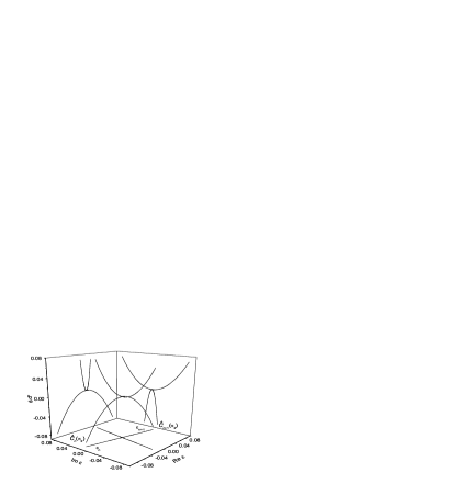
Figure 5: The curves $\hat{C}_{n}(\pi_{2})$ and $\hat{C}_{n+1}(\pi_{2})$ are the intersections of the hyperplane $\pi_{2}$ that goes through the exceptional point $(\xi_{1}^{*},\xi^{*}_{2})$ in parameter space and the two-sheeted surface $\hat{\epsilon}_{1,2}(\xi_{1},\xi_{2})$. The projections of $\hat{C}_{n}(\pi_{2})$ and $\hat{C}_{n+1}(\pi_{2})$ on the planes $(Re{\cal E},\xi_{1})$ and $(Im{\cal E},\xi_{1})$ show a joint crossing of energies and widths. The projections of $\hat{C}_{n}(\pi_{2})$ and $\hat{C}_{n+1}(\pi_{2})$ on the plane $(Re{\cal E},Im{\cal E})$ are the critical trajectories of the $S-$matrix poles in the complex energy plane. At the crossing point, the two simple poles coalesce into one double pole of $S(E)$.

Figure 6: The curves $\hat{C}_{n}(\pi_{3})$ and $\hat{C}_{n+1}(\pi_{3})$ are the intersection of the hiperplane $\pi_{3}:=\bar{\xi}_{2}^{(3)}$ and the two sheeted surface $\hat{\epsilon}_{n,n+1}$. The projections of $\hat{C}_{n}(\pi_{3})$ and $\hat{C}_{n+1}(\pi_{3})$ on the planes (Re ${\cal E},\xi_{1}$) and (Im ${\cal E},\xi_{1}$) show a crossing of energies and an anticrossing of widths. The projections of $\hat{C}_{n}(\pi_{3})$ and $\hat{C}_{n+1}(\pi_{3})$ on the plane $(Re{\cal E},Im{\cal E})$ are the trajectories of the $S-$matrix poles in the complex energy plane and they do not cross. In the figure, $\xi_{1}=d-d^{*}$.

The intersection of the eigenenergy surface $\hat{\epsilon}_{1,2}(\xi_{1},\xi_{2})$ and each one of the hyperplanes $\pi_{i}:\xi_{2}=\bar{\xi}_{2}^{(i)}$, defines two three-dimensional curves for each value of $\bar{\xi}_{2}^{(i)}$

$$\hat{\epsilon}_{1,2}(\xi_{1},\xi_{2})\cap\pi_{i}=\cases{\hat{C}_{1}(\pi_{i})\\ \hat{C}_{2}(\pi_{i})}$$ (49)

The sections $\hat{C}_{1}(\pi_{i})$ and $\hat{C}_{2}(\pi_{i})$ are the three-dimensional curves traced by the points $\hat{\cal E}_{1}(\xi_{1},\bar{\xi}_{2}^{(i)})$ and $\hat{\cal E}_{2}(\xi_{1},\bar{\xi}_{2}^{(i)})$ on the surface $\hat{\epsilon}_{1,2}(\xi_{1},\xi_{2})$ when the point with coordinates $(\xi_{1},\bar{\xi}_{2}^{(i)})$ moves along a straigth line path parallel to the $O\xi_{1}$ axis, and $\xi_{1,i}\leq\xi_{1}\leq\xi_{1,f}$, in parameter space.

The projections of the sections $\hat{C}_{1}(\pi_{i})$ and $\hat{C}_{2}(\pi_{i})$ on the planes (Re $\hat{\cal E},\xi_{1}$) and (Im$\hat{\cal E},\xi_{1}$) are

$$Re[\hat{C}_{m}(\pi_{i})]=Re\hat{\cal E}_{m}(\xi_{1},\bar{\xi}_{2}^{(i)})\hskip 28.45274ptm=1,2$$ (50)

and

$$Im[\hat{C}_{m}(\pi_{i})]=Im\hat{\cal E}_{m}(\xi_{1},\bar{\xi}^{(i)}_{2})\hskip 28.45274ptm=1,2$$ (51)

respectively, see figures 4-6. A comparison of the representations of the eigenenergy surfaces provided by the numerically exact computation and the contact equivalent approximant is shown in figure 7.

The projections of the sections $\hat{C}_{1}(\pi_{i})$ and $\hat{C}_{2}(\pi_{i})$ on the plane $(Re\hat{\cal E}$, Im $\hat{\cal E})$ are the trajectories of the $S-$matrix poles in the complex energy plane. An equation for these trajectories is obtained by eliminating $\xi_{1}$ between Re$\hat{\cal E}_{m}(\xi_{1},\bar{\xi}_{2}^{(i)})$ and Im$\hat{\cal E}_{m}(\xi_{1},\bar{\xi}_{2}^{(i)}),m=1,2,$ equations(44-45),

$$\Bigl{(}Re\hat{\cal E}_{m}\Bigr{)}^{2}-2\cot\phi_{1}\Bigl{(}Re\hat{\cal E}_{m}\Bigr{)}\Bigl{(}Im\hat{\cal E}_{m}\Bigr{)}-\Bigl{(}Im\hat{\cal E}_{m}\Bigr{)}^{2}-\frac{1}{4}\Bigl{(}\vec{R}\cdot\bar{\xi}_{c}^{(i)}\Bigr{)}=0$$ (52)

where

$$\cot\phi_{1}=\frac{R_{2}}{I_{1}}$$ (53)

and the constant vector $\vec{\xi}^{(i)}_{c}$ is such that

$$\Bigl{(}\vec{I}\cdot\vec{\xi}_{c}\Bigr{)}\Bigr{|}_{\xi_{2}=\vec{\xi}^{(i)}_{2}}=0$$ (54)

The discriminant of (52), $4\cot^{2}\phi_{1}+1$, is positive. Therefore, close to the crossing point, the trajectories of the $S-$matrix poles are the branches of a hyperbola defined by (52).

Figure 7: Projections of the sections $\hat{C}_{n}(\pi_{i})$ and $\hat{C}_{n+1}(\pi_{i})$ on the planes (Im ${\cal E},\xi_{1}$) and (Re ${\cal E},\xi_{1}$) are shown in the left and right columns respectively for a) $V_{3}=$ 1.0381, b) $V_{3}=V^{*}_{3}$ and c) $V_{3}=$1.0834. The full line is the numerically exact calculation, the dotted line is the contact equivalent approximant.

4.2 Crossings and anticrossings of energies and widths

Crossings or anticrossings of energies and widths are experimentally observed when the difference of complex resonance energy eigenvalues, $\hat{\cal E}_{1}(\xi_{1},\bar{\xi}_{2})-\hat{\cal E}_{2}(\xi_{1},\bar{\xi}_{2})=\Delta E-i1/2\Delta\Gamma$ is measured as a function of the slowly varying parameter $\xi_{1}$, keeping the other constant, $\xi_{2}=\bar{\xi}_{2}^{(i)}$. From equations (44-45), and keeping $\xi_{2}=\bar{\xi}^{(i)}_{2}$, we obtain

$$\begin{array}[]{c}\Delta E=E_{n}-E_{n+1}=\frac{\sqrt{2}}{2}\Bigl{[}{}_{+}\sqrt{(\vec{R}\cdot\vec{\xi})^{2}+(\vec{I}\cdot\vec{\xi})^{2}}+(\vec{R}\cdot\vec{\xi})\Bigr{]}^{1/2}\Bigr{]}_{\xi_{2}=\bar{\xi}_{2}^{(i)}}\end{array}$$ (55)

and

$$\Delta\Gamma=\Bigl{(}\Gamma_{n}-\Gamma_{n+1}\Bigr{)}=-\sqrt{2}\Bigl{[}{}_{+}\sqrt{(\vec{R}\cdot\vec{\xi})^{2}+(\vec{I}\cdot\vec{\xi})^{2}}-(\vec{R}\cdot\vec{\xi})\Bigr{]}^{1/2}\Bigr{|}_{\xi_{2}=\bar{\xi}_{2}^{(i)}}$$ (56)

These expressions allow us to relate the terms $(\vec{R}\cdot\vec{\xi})$ and $(\vec{I}\cdot\vec{\xi})$ directly with observables of the isolated doublet of resonances. Taking the product of $\Delta E\Delta\Gamma$, and recalling equation (46), we get

$$\Delta E\Delta\Gamma=-\Bigl{(}\vec{I}\cdot\vec{\xi}\Bigr{)}\Bigr{|}_{\xi_{2}=\bar{\xi}_{2}^{(i)}}$$ (58)

and taking the differences of the squares of the left hand sides of (55) and (56), we get

$$\Bigl{(}\Delta E\Bigr{)}^{2}-\frac{1}{4}\Bigl{(}\Delta\Gamma\Bigr{)}^{2}=\Bigl{(}\vec{R}\cdot\vec{\xi}\Bigr{)}\Bigr{|}_{\xi_{2}=\bar{\xi}_{2}^{(i)}}$$ (59)

At a crossing of energies $\Delta E$ vanishes, and at a crossing of widths $\Delta\Gamma$ vanishes. Hence, the relation found in eq.(58) means that a crossing of energies or widths can occur if and only if $(\vec{I}\cdot\vec{\xi})_{\bar{\xi}^{(i)}_{2}}$ vanishes

For a vanishing $(\vec{I}\cdot\vec{\xi}_{c})_{\bar{\xi}^{(i)}_{2}}=0=\Delta E\Delta\Gamma$, we find three cases, which are distinguished by the sign of $(\vec{R}\cdot\vec{\xi}_{c})_{\bar{\xi}^{(i)}_{2}}$. From eqs. (55) and (56),

1. $(\vec{R}\cdot\vec{\xi}_{c})_{\bar{\xi}^{(i)}_{2}}>0$ implies $\Delta E\neq 0$ and $\Delta\Gamma=0$, that is, energy anticrossing and width crossing.

2. $(\vec{R}\cdot\vec{\xi}_{c})_{\bar{\xi}^{(i)}_{2}}=0$ implies $\Delta E=0$ and $\Delta\Gamma=0$, that is, joint energy and width crossings, which is also degeneracy of the two complex resonance energy eigenvalues.

3. $(\vec{R}\cdot\vec{\xi}_{c})_{\bar{\xi}^{(i)}_{2}}<0$ implies $\Delta E=0$ and $\Delta\Gamma\neq 0$, i.e. energy crossing and width anticrossing.

This rich physical scenario of crossings and anticrossings for the energies and widths of the complex resonance energy eigenvalues extends a theorem of von Neumann and Wigner [5] for bound states to the case of unbound states.

The general character of the crossing-anticrossing relations of the energies and widths of a mixing isolated doublet of resonances, discussed above, has been experimentally established by P. von Brentano and his collaborators in a series of beautiful experiments [48, 49, 50].

4.3 Trajectories of the $S-$matrix poles and changes of identity

In subsection 4.1, we found that, when one control parameter, say $\xi_{1}$, is varied and the other control parameter is kept constant $\bar{\xi}^{(i)}_{2}$ and close to the exceptional value, the trajectories of the $S-$matrix poles are the branches of a hyperbola defined by (52-54). The asymptotes of this hyperbola are the two straight lines defined by

$$Im{\cal E}^{(I)}=\tan\frac{\phi}{2}Re{\cal E}^{(I)}$$ (60)

and

$$Im{\cal E}^{(II)}=-\cot\frac{\phi}{2}Re{\cal E}^{(II)}$$ (61)

The two branches of the hyperbola are in opposite quadrants of the complex energy plane divided by the asymptotes, see figure 8.

Figure 8: Trajectories of the poles of the scattering matrix, $S({\cal E})$, of an isolated doublet of resonances in a double barrier potential close to a degeneracy of unbound states. The control parameters are the width, $d$, of the inner barrier and the depth, $V_{3}$, of the outer well. The trajectories are traced by the poles ${\cal E}_{1}(d,V^{(i)}_{3})$ and ${\cal E}_{2}(d,V^{(i)}_{3})$ on the complex ${\cal E}-$plane when the point $(d,V^{(i)}_{3})$ moves on the straight line path $\pi_{i}$; $V_{3}=V^{(i)}_{3}$. The top, middle, and bottom figures show the trajectories corresponding to $(\vec{R}\cdot\vec{\xi}_{c})_{\bar{\xi}^{(i)}_{2}}>0$, $(\vec{R}\cdot\vec{\xi}_{c})_{\bar{\xi}^{(i)}_{2}}=0$, and $(\vec{R}\cdot\vec{\xi}_{c})_{\bar{\xi}^{(i)}_{2}}<0$, respectively, with $(\xi_{1},\xi_{2})=(d-d^{*},V_{3}-V^{*}_{3})$. The full line is the numerically exact calculation, the dotted line is the contact equivalent approximant.

We find three types of trajectories, which are distinguished by the sign of $(\vec{R}\cdot\vec{\xi})|_{\xi_{2}=\bar{\xi}_{2}}$:

1. When $(\vec{R}\cdot\vec{\xi})|_{\xi_{2}=\bar{\xi}_{2}}>0$, one branch of the hyperbola lies to the left and the other lies to the right of a vertical line that goes through the crossing point.

2. Critical trajectories, when $(\vec{R}\cdot\vec{\xi})|_{\xi_{2}=\bar{\xi}_{2}}=0$, the trajectories are the asymptotes of the hyperbola. The two simple poles start from opposite ends of the same straight line and move towards each other until they meet at the crossing point where they coalesce to form a double pole of the $S-$matrix. From there, they separate moving away from each other on a straight line at $90^{\circ}$ with respect to the first asymptote.

3. When $(\vec{R}\cdot\vec{\xi})|_{\xi_{2}=\bar{\xi}_{2}}<0$, one pole moves on one branch of the hyperbola that lies above and the other pole moves on the other branch that lies below a horizontal straight line that goes through the crossing point.

Figure 9: The two poles of the isolated doublet of unbound states trace a starlike trajectory in the complex $k-$plane, shown on the left hand side of the figure, when the physical system is transported in parameter space twice around the exceptional point in the circular path shown at the right hand side of the figure. For an explanation, see the text.

When a small change in the control parameter $\bar{\xi}_{2}^{(i)}$ changes the sign of $(\vec{R}\cdot\vec{\xi})|_{\xi_{2}=\bar{\xi}_{2}}$, it produces a small change in the initial position of the poles, but the trajectories change suddenly from type (i) to type (iii), this very large and sudden change of the trajectories exchanges almost exactly the final position of the poles as can be appreciated from figure 8. This dramatic change was called a “change of identity” by Vanroose, van Leuven, Arickx and Broeckhove [8] who discussed an example of this phenomenon in the $S-$matrix poles in a two-channel model, Vanroose [51] has also discussed these properties in the case of the scattering of a beam of particles by a double barrier potential with two regions of trapping.

4.4 Changes of identity when going around the exceptional point

In the previous discussion of the trajectories of the $S-$matrix poles and their changes of identity, the two straight lines, parallel to the $O\xi_{1}$ axis, defined by the conditions $\xi_{1,i}\leq\xi_{1}\leq\xi_{1,f}$ and $\xi_{2}=\bar{\xi}^{(i)}_{2}$, i = 1,3, are the two long sides of a very long and narrow rectangle in parameter space that surrounds the exceptional point. The two short sides of this rectangle are defined by the small change in $\xi_{2}$ when going from $\bar{\xi}^{(1)}_{2}$ to $\bar{\xi}^{(3)}_{2}$, keeping $\xi_{1,i}$ or $\xi_{1,f}$ constant, to which we refered above, when explaining the changes of identity of the poles of the doublet of unbound states. In order to understand better the meaning of the changes of identity of those poles, it will be convenient to deform continuously the long and narrow rectangle into a circle and consider the motion of the zeroes of the Jost function $k_{1}(x_{1},x_{2})$ and $k_{2}(x_{1},x_{2})$ in the complex $k-$plane, when the system is transported in parameter space around the exceptional point in the closed circular path equivalent by continuous deformation to the long and narrow rectangle of the previous discussion.

On the left hand side of figure 9, we show the trajectory traced in the complex $k-$plane by the two zeroes of the Jost function, $k_{1}(x_{1},x_{2})$ and $k_{2}(x_{1},x_{2})$, when the physical system is transported in parameter space twice around the exceptional point on the double circular circuit shown on the right hand side of the same figure. When the system is at the crossing point of the two circular paths in parameter space, one zero, say $k_{1}(x_{1},x_{2})$, is at the uppermost point and the other, say $k_{2}(x_{1},x_{2})$, is at the lowermost point of the four points star in the complex $k-$plane.

1. As the point representing the system in parameter space moves on the inner circle in counterclockwise direction, from its initial position until it makes one complete round about the exceptional point and is back at its initial position, the $k_{1}(x_{1},x_{2})$ zero moves on the star in the complex $k-$plane in clockwise direction, from its initial position at the topmost point of the star, goes through the point at the extreme right hand side of the star and ends at the lowest point in the star, while the $k_{2}(x_{1},x_{2})$ zero moves also in clockwise direction, from its initial position at the lowest point in the star goes trough the point in the extreme left hand side of the star and ends at topmost point on the star. It follows that, when the system goes around the exceptional point once in parameter space, the poles of the scattering matrix are exactly exchanged.

2. As the point representing the system in parameter space continues its conterclockwise motion, now on the outercircle, until it completes a second round about the exceptional point and is back at its initial position, the $k_{1}(x_{1},x_{2})$ zero moves on the star in the complex $k-$plane in clockwise direction from the lowest point on the star, goes through the extreme left hand side point on the star and ends at the topmost point on the star, while the $k_{2}(x_{1},x_{2})$ zero moves on the star in the complex $k-$plane also in clockwise direction, from the topmost point on the star, goes through the extreme right hand side point on the star and ends at lowest point of the four points star. Therefore, when the system goes around the exceptional point twice in parameter space the poles of the $S(k)$ matrix and the complex energy eigenvalues return to their initial values in the complex $k-$plane. The eigenfunctions also return to their initial values but they acquire a geometric phase [27, 28, 29, 30, 31, 52].

5 Summary and conclusion

In this paper, we discussed some mathematical and physical aspects of the non-Hermitian degeneracy of two unbound energy eigenstates of a Hamiltonian dependending on two control parameters. We solved numerically the implicit transcendental equation that defines the eigenenergy surface of a degenerating isolated doublet of unbound states in the simple but illustrative case of the scattering of a beam of particles by a double square barrier potential. The analytical characterization of the singularity of the energy surface was made in the more general case of a short ranged potential with two regions of trapping. We showed that, from the explicit knowledge of the Jost function as a function of the control parameters of the system, it is possible to derive a two parameter family of functions which is contact equivalent to the exact energy-pole position function at the degeneracy point and includes all small perturbations of the degeneracy conditions. This unfolding of the degeneracy point gives a simple and explicit, but very accurate, representation of the eigenenergy surface close to the exceptional point, see figure 7. In parameter space, the surface that represents the complex energy eigenvalues has a branch point of square root type at the crossing point, and branch cuts in its real and imaginary parts that start at the exceptional point but extend in opposite directions in parameter space. In the complex energy plane, the crossing point of two simple resonance poles of the scattering matrix is an isolated point where the scattering matrix has one double resonance pole. Crossings and anticrossings of the energies and widths of the resonances in an isolated doublet of unbound states of a quantum system, as well as the sudden change in the shape of the $S-$matrix pole trajectories, observed when one control parameter is varied while the other is kept constant at a value close to the exceptional value, are fully explained in terms of sections of the energy surfaces.

6 Acknowledgements

We thank Professor Peter von Brentano (Universität zu Köln) for many inspiring discussions on this exciting problem. This work was partially supported by CONACyT México under Contract No. 40162-F and by DGAPA-UNAM Contract No. PAPIIT:
IN116202

References

References

- [1] Gamow G 1928 Z. Phys 51 204
- [2] Peierls R E 1959 Proc. Roy. Soc. (London) Ser. A 253 16
- [3] Hernández E, Jáuregui A, and Mondragón A 2003 Phys. Rev. A 67 022721
- [4] Berry M V 2004 Czech. J. Phys. 54 1039
- [5] von Neumann J and Wigner E P 1929 Physik Z. 30 467
- [6] Teller E 1937 J. Phys. Chem. 41 109
- [7] von Brentano P 1990 Phys. Lett. B 238 1; 1990 Phys. Lett. B 246 320; 1991 Phys. Lett. B 26514
- [8] Vanroose W, Leuven P, Arickx F, and Broeckhove J 1997 J. Phys. A: Math. Gen. 30 5543
- [9] Friedrich H and Wintgen D 1985 Phys. Rev. A 32 3231
- [10] Mondragón A, and Hernández E 1993 J. Phys. A: Math. Gen. 26 5595
- [11] Hernández E and Mondragón A (1994) Phys. Lett. B 326 1
- [12] von Brentano P 1996 Phys. Rep. 264 57
- [13] Antoniou I, Gadella M and Pronko G 1998 J. Math. Phys. 39 2429
- [14] Bohm A, Loewe M, Maxson S, Patuleanu, Püntmann C and Gadella M 1997 J. Math. Phys. 38 6072
- [15] Lassila K E and Ruuskanen V 1966 Phys. Rev. Lett. 17 490
- [16] Knight P L 1979 Phys. Lett. A 72 309
- [17] Kylstra N J and Joachain C J 1996 Europhys. Lett. 36 657
- [18] Kylstra N J and Joachain C J 1998 Phys. Rev. A 57 412
- [19] Znojil M 2006 J. Phys A: Math. Gen. 39 441
- [20] Znojil M 1999 Phys. Lett. A 259 220
- [21] Znojil M Levai G, 2001 Mod. Phys. Lett. A 16 2273
- [22] Mostafazadeh A 2002 J. Math. Phys. 43 6443
- [23] Rotter I, Sadreev A F 2005 Phys. Rev. E 71 036227
- [24] Rotter I 2003 Phys. Rev. E 67 026204
- [25] Rotter I 2002 Phys. Rev. E 65 026217
- [26] Magunov A L, Rotter I, Strakhova S I 2001 J. Phys B: Atom. Mol. Opt. Phys. 34 29
- [27] Hernández E, Jáuregui A, and Mondragón A 1992 Rev. Mex. Fis. 38, Suppl 2, 128
- [28] Mondragón A and Hernández E 1996 J. Phys. A: Math. Gen. 29 2567
- [29] Mondragón A and Hernández E 1998 Accidental degeneracy and Berry phase of resonant states Irreversibility and Causality: Semigroups and Rigged Hilbert Sapce (Lecture Notes in Physics) vol 504 Ed A. Bohm, H-D Doebner and P Kielanowski (Berlin: Springer-Verlag) p 257
- [30] Heiss W D 1999 Eur. Phys. J. D 7 1
- [31] Mailybaev Alexei A, Kirillov Oleg N and Seyranian Alexander P 2005 Phys. Rev. A 72 014104
- [32] Dembowski C, Gräf H D, Harney H L, Heine A, Heiss W D, Rehfeld H and Richter A 2001 Phys. Rev. Lett. 86 787
- [33] Dembowski C, Dietz B, Gräf H D, Harney H L, Heine A, Heiss W D, and Richter A 2003 Phys. Rev. Lett. 90 034101
- [34] Hernández E, Jáuregui A, and Mondragón A 2005 Phys. Rev. E 72 026221
- [35] Berry M V and Dennis M R 2003 Proc. R. Soc. Lond. A 459 1261
- [36] Keck F, Korsch H J, and Mossmann S 2003 J. Phys. A: Math. Gen. 36 2125
- [37] Korsch H J, and Mossmann S 2003 J. Phys. A: Math. Gen. 36 2139
- [38] Shuvalov A L and Scott N 2000 Acta Mech. 140 1
- [39] Seyranian A P, Kirillov O N and Mailybaev A A 2005 J. Phys. A: Math. Gen. 38 1723
- [40] Kirillov O N, Mailybaev A A and Seyranian A P 2005 J. Phys. A: Math. Gen. 38 5531
- [41] Stehmann T, Heiss W D, Scholtz F G 2004 J. Phys. A: Math. Gen. 37 7813
- [42] Heiss W D, 2004 J. Phys. A: Math. Gen. 37 2455
- [43] Newton R G 1982 Scattering Theory of Waves and Particles, 2nd. edn. (Berlin: Springer-Verlag) Chapt. 12
- [44] Boas R P 1954 Entire Functions (Academic New York) p. 22
- [45] Pfluger A 1943 Communs. Math. Helv. 16 1
- [46] Krantz S G and Parks H R 2002 The Implicit Function Theorem (Boston:Birkhäuser) Chapt. 5
- [47] Seydel R 1991 Practical Bifurcation and Stability Analysis. IAM5 2nd. edn. (New York: Springer-Verlag) Chapt. 8
- [48] von Brentano P, and Philipp M 1999 Phys. Lett. B 454 171
- [49] Philipp M, von Brentano P, Pascovici G and Richter A 2000 Phys. Rev. E 62 1922
- [50] von Brentano P 2000 Rev. Mex. Fis48, Suppl 2, 1
- [51] Vanroose W 2001 Phys. Rev. A 64 062708
- [52] Berry M V 1984 Proc. R. Soc. (London) A 392 45