Transport dynamics of single ions in segmented microstructured Paul trap arrays

Abstract.

It was recently proposed to use small groups of trapped ions as qubit carriers in miniaturized electrode arrays that comprise a large number of individual trapping zones, between which ions could be moved [1, 2]. This approach might be scalable for quantum information processing with a large numbers of qubits. Processing of quantum information is achieved by transporting ions to and from separate memory and qubit manipulation zones in between quantum logic operations. The transport of ion groups in this scheme plays a major role and requires precise experimental control and fast transport. In this paper we introduce a theoretical framework to study ion transport in external potentials that might be created by typical miniaturized Paul trap electrode arrays. In particular we discuss the relationship between classical and quantum descriptions of the transport and study the energy transfer to the oscillatory motion during near-adiabatic transport. Based on our findings we suggest a numerical method to find electrode potentials as a function of time to optimize the local potential an ion experiences during transport. We demonstrate this method for one specific electrode geometry that should closely represent the situation encountered in realistic trap arrays.

1. Introduction

Quantum information processing is a rapidly evolving field of physical science. Its practical importance arises from the exponential speedup in computation of certain algorithmic tasks over classical computation [3]. Building an actual device that can process quantum information, however, is technologically difficult due to the need for qubits that can be processed and read out with high fidelities and the extreme sensitivity of the quantum mechanical states stored in these units against external uncontrolled perturbations. A promising technical approach as shown over the last decade, is to use strings of ions as physical qubits confined in linear electromagnetic Paul traps [1, 4]. These strings are stored in a single trap and constitute a one dimensional crystallized structure whose vibrational modes can be laser cooled to their ground states. The strong mutual coupling of the ions by Coulomb forces in such a crystal has been proposed and utilized to create arbitrary superpositions of quantum states of the ionic internal states ([4, 5, 6]). In the last few years methods were developed that enable quantum state engineering with high precision and long coherence times [7, 8, 9, 10, 11]. The necessary criteria [12] for large-scale quantum computation have been demonstrated in the past years, and small algorithms have been implemented successfully [13, 14, 15, 16, 17]. However, as in other approaches aiming towards quantum computation, scaling to many qubits is challenging. Considerable overhead is required by quantum error correcting schemes that permit robust quantum computation and make large-scale implementations feasible. To scale up a linear string of many ions, a rapidly growing number of vibrational degrees of freedom needs to be controlled and cooled to the ground state for reliable processing. This is extremely difficult to realize. A more recent proposal [1, 2] has been made to circumvent this problem by using small arrays of a few qubits that are shuttled around in two-dimensional microstructures to process and store quantum states at various locations.

An initial systematic study showed that coherent transport of ions in linear trap arrays is possible with nearly no loss in contrast during the motion [18]. In this experiment an adiabatic transport of a qubit was performed over a distance of $1.2~{}mm$ in a time span of about $54~{}\mu s$ with negligible heating. Currently, there are strong efforts under way to demonstrate the possibility of building large-scale ion trap structures. For example, suggestions have been made to combine miniaturized ion chips directly with CMOS electronics to handle the resources required to control the many electric potentials [19]. Moreover, fast transport requires excellent experimental control of all these potentials.

A detailed scheme of how a viable architechture of an ion trap processor could look has been recently studied by Steane [20], fully incorporating quantum error correcting codes. The physical gate rate of this proposed 300 qubit processor unit was found to be limited by

$$\tau_{g}=\frac{2}{\nu_{\text{COM}}}+\frac{10}{\nu_{\text{r}}}+\tau_{\text{cool}}+\tau_{p}\sim\text{a few}\ \mu s,$$ (1)

with the first two terms being an average time of the part of a typical gate that involve motion that is times for splitting ($\sim 2\nu_{\text{COM}}^{-1}$), recombining and moving ($\sim 10\nu_{\text{r}}^{-1}$) a small ion string, where $\nu_{\text{COM}}$ and $\nu_{\text{r}}$ are typical axial and radial trapping frequencies, respectively. The last two terms correspond to cooling after the transport has been done, and the time duration of conducting the actual phase gate, respectively. On the other hand, if large amounts of energy are transferred to the ions, longer cooling times might be needed. Inserting typical operating conditions shows that the first two terms make up a considerable part of the performance of the physical gate rate. In order to keep this part as small as possible we need designs for electrode structures enabling fast qubit transport.

In the following we present a theoretical framework that governs the transport dynamics of ions trapped in a time varying external potential. In Sect. 2 the equations of motion for the transport are derived. Sect. 3 discusses the general classical solution in terms of an Ermakov parametrization. This approach is useful to express the quantum approach presented in Sect. 5, which uses the Heisenberg picture following the approach of Kim et al. [21]. In Sect. 4 we point out some well-known properties of a quantum harmonic oscillator exposed to a transporting force for the simpler case when its frequency is kept constant. Sect. 5 presents the general quantum solutions and the interrelation between classical and quantum transport. Based on this framework we discuss in Sect. 6 a well-controlled regime for the transport and also include first order perturbations to the transport dynamics. In Sect. 7, we present numerical optimization routines to extract optimum switching of potentials for the transport and study miniaturization of electrode structures to estimate the required resources for a well-controlled transport. Finally, a simple electrode model is used to find a practical rule for the segmentation of ion traps revealing insight into the resources needed for large-scale layouts, that should be also applicable for more general trap arrays.

2. Classical equations of motion

A linear segmented Paul trap, e.g. as used in recent experiments [5, 14, 15, 16, 22, 23], consists typically of two alumina wafers with gold coated electrode surfaces of a few micrometer thickness. The slotted wafers provide electrical RF and DC fields for 3D confinement of ions. The arrangement for control electrodes is schematically sketched in Fig.3 where only a single layer is shown. The confinement along the $x$-axis is achieved solely by electrostatic fields whereas the remaining two orthogonal radial directions correspond to a dynamical trapping by ponderomotive RF forces. In this article we limit ourselves to transport along a single dimension $x$ from $-b/2$ to $b/2$. If we denote the coordinate of the ion in the laboratory frame by $q$ then we have from Newton’s equation of motion

$$\ddot{q}(t)+\frac{Q}{m}\frac{\partial\phi(q,t)}{\partial q}=0,\qquad q(-t_{0})=-\frac{b}{2},\quad\dot{q}(-t_{0})=0,$$ (2)

with two initial conditions as the equations on the rhs; $Q$ is the elementary charge and $m$ the mass of the transported ion. We assume a time interval and location of the ion starting at $-t_{0}$ and $-b/2$, and ending at $+t_{0}$ and $b/2$, respectively. In order to make use of coherent states of a harmonic oscillator (that do not spread in time) we are interested in designing the time-dependent electrical potential as

$$\phi(q,t)\sim\phi_{\text{local}}(q-q_{0}(t))+\varphi_{0}(t),$$ (3)

where $\phi_{\text{local}}(q)\sim m\omega_{0}^{2}q^{2}/2Q$ is purely quadratic with constant curvature in a sufficiently large range around the minimum, and $\varphi_{0}(t)$ is a time-dependent offset with no influence on the dynamics. Here, we prescribe the dynamics by specifying a desired harmonic frequency $\omega_{0}$ and the temporal shift of the harmonic well by a transport function $q_{0}(t)$. The residual, uncontrolled force caused by insufficient flexibility in creating the desired harmonic potential deteriorates the transport performance. Its effect can be described by the difference potential or residual acceleration, i.e.

$$\phi_{\text{res}}(q,t)=\phi(q,t)-\varphi_{0}(t)-\frac{m\omega_{0}^{2}(q-q_{0}(t))^{2}}{2Q}\qquad\text{and}\qquad a_{\text{res}}(q)=-\frac{Q}{m}\frac{\partial\phi_{\text{res}}(q)}{\partial q},$$ (4)

respectively. Due to imperfect realization of the harmonic well $\phi_{\text{res}}(q,t)$ adds fluctuating parts to the ideal harmonic potential as a function of position or time, critically depending on the electrode structure used. In section 7 we will discuss a numerical scheme for approximating $\phi(q,t)$ based on superpositions of individual electrode potentials in an optimal way.

We finally can write down the classical equation of motion

$$\ddot{u}+\omega_{0}^{2}u=-\ddot{q}_{0}(t)+a_{\text{res}}(u+q_{0}(t))$$ (5)

which we transformed into a frame moving with $q_{0}(t)$ by $u=q-q_{0}$. The net acceleration on the rhs corresponds to an external force and displaces the ion from its equilibrium position $u=0$ in this frame. Since we will treat only the first two perturbation terms we expand the final equation of motion around the minimum of the well and rearrange some terms to get

$$\ddot{u}+\omega_{0}^{2}\Bigl{(}1-a^{\prime}_{\text{res}}[q_{0}(t)]/\omega_{0}^{2}\Bigr{)}u-a^{\prime\prime}_{\text{res}}[q_{0}(t)]/2~{}u^{2}+\ldots=-\ddot{q}_{0}(t)+a_{\text{res}}[q_{0}(t)]$$ (6)

where primes denote differentiation with respect to $u$. For the following discussion we abbreviate $\omega^{2}(t)=\omega_{0}^{2}(1-a^{\prime}_{\text{res}}[q_{0}(t)]/\omega_{0}^{2})$ and write $f(t)=-\ddot{q}_{0}(t)+a_{\text{res}}[q_{0}(t)]$ for the rhs of Eq.(6). For certain electrode structures, we can disregard terms involving the second and higher order derivatives of $a_{\text{res}}(q)$ (cf. Section 7). We will make this assumption throughout the paper. In that case Eq.(6) simplifies to the equation of motion of a parametrically driven and forced harmonic oscillator with the Hamiltonian

$${\cal H}(t)=\frac{p^{2}}{2m}+\frac{m\omega^{2}(t)}{2}u^{2}-mf(t)u$$ (7)

and $p=m\dot{u}$.

3. Classical dynamics of ion transport

To obtain a general classical solution with an arbitrary frequency modulation we first consider the formalism which is most often used in conjunction with time-dependent invariants within so called Lewis-Riesenfeld methods [30]. These approaches have been shown to be successful in the quantization of time-dependent harmonic oscillators with many different kinds of time-dependencies. Here, we discuss the general classical solution using the Ermakov equation and its generalized phase equation for time-dependent frequencies. We then employ in section 5 the approach of Kim et al. [21] to express the general quantum solution in terms of its classical solution.

3.1. Homogeneous Solution

Neglecting higher order terms we find the homogeneous part of the solution of Eq.(6) by setting $f(t)=0$, thus solving

$$\ddot{u}_{c}+\omega^{2}(t)u_{c}=0$$ (8)

for an arbitrary time-dependent frequency $\omega(t)$. For this, it is most convenient to make the ansatz

$$u_{1}=\rho(t)e^{i\mu(t)}\qquad u_{2}=\rho(t)e^{-i\mu(t)},$$ (9)

introducing an amplitude function $\rho(t)$ and a phase function $\mu(t)$, both real. Inserting Eq.(9) into Eq.(8) and considering real and imaginary parts results in the two equations

$$\ddot{\rho}-\rho\dot{\mu}^{2}+\omega^{2}(t)\rho=0,\qquad 2\dot{\rho}\dot{\mu}+\rho\ddot{\mu}=0.$$ (10)

$\rho$ is an integrating factor for the second equation on the right so that we can write

$$\qquad\rho^{2}\dot{\mu}=1,$$ (11)

where we have chosen the integration constant as $1$. The constant on the rhs of Eq.(11) has the SI units $m^{2}~{}rad/s$ that should be taken into account at the end. If we substitute this back into the first equation of Eq.(10) we obtain the Ermakov equation for the amplitude function $\rho(t)$

$$\ddot{\rho}+\omega^{2}(t)\rho=1/\rho^{3}.$$ (12)

For periods of constant frequency $\omega=\omega_{0}$ the general solution is

$$\rho(t)=\pm\omega_{0}^{-1/2}\sqrt{\cosh\delta+\sinh\delta\sin(2\omega_{0}t+\theta)},$$ (13)

where $\delta,\theta$ are constants of integration, their values depend on the past evolution [30]. The solution for the generalized phase is easily obtained once $\rho$ is known. From Eq.(11) we have

$$\mu(t)=\int^{t}_{-t_{0}}dt^{\prime}\rho(t^{\prime})^{-2}.$$ (14)

The general homogeneous solution is then given by

$$u_{h}(t)=a_{c}\rho(t)\cos(\mu(t)+\varphi),$$ (15)

with the classical amplitude $a_{c}$ and initial phase $\varphi$ fixed by the initial conditions.

3.2. Green’s function and general solution

We use the general framework of Green’s functions to define a particular solution to the inhomogeneous case of Eq.(6), where we again terminate the expansion, i.e. $a_{\text{res}}^{(n)}[q]=0$ for $n\geq 2$, to stay in a harmonic regime. Using the two independent homogeneous solutions of Eq.(9) we can determine the causal Green’s function

$$G(t,t^{\prime})=\theta(t-t^{\prime})\rho(t)\rho(t^{\prime})\sin(\mu(t)-\mu(t^{\prime})),$$ (16)

with $\theta(t-t^{\prime})$ the Heaviside function. Employing $G(t,t^{\prime})$, a particular solution is given by

$$u_{p}(t)=\int_{-t_{0}}^{t}dt^{\prime}G(t,t^{\prime})f(t^{\prime})=\rho(t)\int_{-t_{0}}^{t}dt^{\prime}\sin(\mu(t)-\mu(t^{\prime}))\rho(t^{\prime})f(t^{\prime}).$$ (17)

For later convenience we define the auxiliary function $\zeta(t)=ie^{-i\mu(t)}\int dt^{\prime}e^{i\mu(t^{\prime})}\rho(t^{\prime})f(t^{\prime})$ which will be useful for expressing the general quantum solution. In this notation we can abbreviate the particular solution by $u_{p}(t)=\rho(t)\left\{\zeta(t)+\zeta^{*}(t)\right\}/2$.

Thus, we obtained the general solution as the sum of the general homogeneous solution Eq.(15) and a particular solution

$$u_{c}(t)=u_{\text{h}}(t)+u_{p}(t)\equiv\rho(t)/2\left\{a_{c}e^{i(\mu(t)+\varphi)}+\zeta(t)\right\}+c.c.\quad.$$ (18)

Higher derivatives, like velocity and acceleration, can easily be found from the general solution in Eq.(18) by using the Leibniz rule. For initial conditions where we start in the classical ground state $a_{c}=0$ we define the quantity $\Xi(t)=\dot{u}_{p}(t)+i\omega(t)u_{p}(t)$, assuming that the transport starts at $-t_{0}>-\infty$, i.e. later than the infinite past, and demand that it takes a finite amount of time. With the help of the last definition the energy transferred to the oscillator at instants $t_{1}$ (where $f(t_{1})\equiv 0$) is then given by

$${\cal W}(t_{1})=m\left|\Xi(t_{1})\right|^{2}/2,$$ (19)

with

$$\Xi(t_{1})=\int_{-t_{0}}^{t_{1}}dt^{\prime}\rho(t^{\prime})\Bigl{(}\rho(t_{1})\dot{\mu}(t_{1})\cos(\Delta\mu_{1t^{\prime}})+\{\dot{\rho}(t_{1})+i\omega(t_{1})\rho(t_{1})\}\sin(\Delta\mu_{1t^{\prime}})\Bigr{)}f(t^{\prime}),$$ (20)

and $\Delta\mu_{1t^{\prime}}=\mu(t_{1})-\mu(t^{\prime})$. We will call $\Xi(t)$ the adiabatic suppression amplitude and its absolute square the adiabatic suppression factor. Thus, we have derived the classical energy transfer for arbitrary frequency evolutions and arbitrary external transport forces. To evaluate this expression one first must solve for the explicit time-dependence of $\rho$ and $\mu$ according to Eqs.(12,14) by integrating the Ermakov equation and the phase equation, and finally compute the transferred energy at different times using Eqs.(19,20).

3.3. Adiabatic limit

Since we are mainly interested in an adiabatic solution we can simplify the last expression by considering adiabatic expansions of the homogeneous solution for a parametrically driven harmonic oscillator. We introduce an adiabatic time scale ${\cal T}$ such that

$$\dot{\omega}/\omega\sim{\cal T}^{-1}\quad\text{for}\quad{\cal T}\gg\omega^{-1}.$$ (21)

The general adiabatic expansion of the differential equations Eqs.(12,14) is readily obtained [29]

$$\rho(t)\sim\frac{1}{\sqrt{\omega(t)}}+\frac{1}{8}\frac{\ddot{\omega}(t)}{\omega(t)^{7/2}}-\frac{3}{16}\frac{\dot{\omega}(t)^{2}}{\omega(t)^{9/2}}+\cdots\quad\text{and}\quad\dot{\mu}(t)\sim\omega(t)-\frac{1}{4}\frac{\ddot{\omega}(t)}{\omega(t)^{2}}+\frac{3}{8}\frac{\dot{\omega}(t)^{2}}{\omega(t)^{3}}+\cdots$$ (22)

This procedure is equivalent to a perturbative approach on the first term in Eq.(12) [30]. We require that at instants $-t_{0},t_{1}$, i.e. at times when we measure the oscillator’s energy, the frequency has settled into a constant. Also for the following discussion we define that the oscillator’s initial frequency at $-t_{0}$ is $\omega(-t_{0})=\omega_{0}$, so that $\rho(-t_{0})=1/\sqrt{\omega_{0}}$, $\dot{\rho}(-t_{0})=0$. Taking into account only the lowest order of the expansion in Eq.(22) the expression in Eq.(20) reduces to

$$\Xi(t_{1})=\sqrt{\omega(t_{1})}\int_{-t_{0}}^{t_{1}}dt^{\prime}f(t^{\prime})\omega(t^{\prime})^{-1/2}e^{i\Delta\mu_{1t^{\prime}}}\qquad \text{with}\quad\Delta\mu_{1t^{\prime}}=\int_{t^{\prime}}^{t_{1}}d\tau\ \omega(\tau)$$ (23)

providing the adiabatic energy transfer in the first order of frequency modulation.

4. Quantum and classical, dragged harmonic oscillators with constant frequency

Husimi [27] and Kerner [28] independently considered the forced quantum mechanical oscillator and found exact analytical expressions for their wavefunctions and propagators. We review some of their early ideas because they provide insight into the close relationship of the quantum and classical solution. In this paragraph we assume the frequency is independent of time. The corresponding Hamiltonian is given by Eq.(7) with $\omega(t)=\omega_{0}$.

Following Husimi and Kerner, we can ”uncouple” the classical oscillation by the transformation

$$\Psi(u,t)=\phi(u^{\prime},t)\exp(im\dot{u}_{c}u^{\prime}/\hbar),$$ (24)

with $u^{\prime}=u-u_{c}$ and $u_{c}$ at first undefined. Inserting Eq.(24) into the time-dependent Schrödinger equation gives

$$i\hbar\frac{\partial\phi}{\partial t}=\left(-\frac{\hbar^{2}}{2m}\frac{\partial^{2}}{\partial u^{\prime 2}}+\frac{1}{2}m\omega_{0}^{2}u^{\prime 2}\right)\phi+m(\ddot{u}_{c}+\omega_{0}^{2}u_{c}-f)u^{\prime}\phi-(m/2)(\dot{u}_{c}^{2}-\omega_{0}^{2}u_{c}^{2}+2fu_{c})\phi.$$ (25)

On the rhs we see that we can make the second term vanishing if we choose $u_{c}$ to satisfy

$$\ddot{u}_{c}+\omega_{0}^{2}u_{c}-f=0,$$

i.e. if $u_{c}$ satisfies the classical solution of Eq.(7). With this choice one can easily identify the classical action $L(t)=(m/2)(\dot{u}_{c}^{2}-\omega^{2}u_{c}^{2}+2fu_{c})$ of a forced harmonic oscillator in the third term on the rhs of Eq.(25). Furthermore, if we make the ansatz

$$\phi(u^{\prime},t)=\chi(u^{\prime},t)\exp\left[{\frac{i}{\hbar}\int_{-\infty}^{t}dt^{\prime}L(t^{\prime})}\right],$$

we can absorb this term as a time-dependent phase into $\phi$. The remaining part of the wavefunction, $\chi$, then needs only to obey the usual harmonic oscillator wave equation in the frame defined by the classical trajectory with its internal coordinate $u^{\prime}$

$$i\hbar\frac{\partial\chi}{\partial t}=\left(-\frac{\hbar^{2}}{2m}\frac{\partial^{2}}{\partial u^{\prime 2}}+\frac{1}{2}m\omega_{0}^{2}u^{\prime 2}\right)\chi.$$ (26)

In this way one can achieve a separation of the forced harmonic oscillator from the unforced oscillator in a frame moving with the classial trajectory. The wavepacket does not become deformed by the homogeneously acting force. The quantum solution becomes displaced and only a phase is accumulated.

To determine further properties we can assume now a stationary state with energy $\epsilon_{n}$ for the solution of Eq.(26)

$$\chi_{n}(u^{\prime},t)=u_{n}(u^{\prime})\exp(-i\epsilon_{n}t)\qquad\epsilon_{n}=(n+\tfrac{1}{2})\hbar\omega_{0},$$

and evaluate transition probabilities at time $t$ for the oscillator to be in the number state $u_{m}$ if it was initially in the number state $u_{n}$

$$P_{mn}(t)=\left|\int_{-\infty}^{\infty}u_{m}(u-u_{c}(t))u_{n}(u)e^{im\dot{u}_{c}(t)u/\hbar}du\right|^{2}.$$

Husimi and Kerner showed that these transition moments can be evaluated analytically

$$P_{mn}(t)=(\mu!/\nu!)\gamma^{\nu-\mu}e^{-\gamma}(L_{\mu}^{\nu-\mu}(\gamma))^{2}\qquad\text{with}\quad\gamma(t)=m/2\hbar\omega_{0}~{}|\dot{u}_{c}+i\omega u_{c}|^{2}$$ (27)

by using generating functions for the Hermite polynomials [27, 28]. In Eq.(27), $\nu$ is the greater while $\mu$ is the lesser of $m$ and $n$, respectively. $L_{\mu}^{\nu-\mu}$ denote the associated Laguerre polynomials, and its time-dependent argument $\gamma(t)$ describes the classical energy transfer in units of $\hbar\omega_{0}$. From Eq.(27) we see the classical character of the quantum solution: the transition probabilities are solely defined by the classical quantity $\gamma(t)$. Also, if we consider starting from the ground state $n=\mu=0$ and using $L_{0}^{\nu}(\gamma)\equiv 1$ the probability distribution $P_{m0}$ becomes a poissonian, and thus we find the signature of a coherent state.

With this relation the expectation values for the mean energy and the dispersion of the energy distribution are then immediately obtained

$$\langle E_{m}\rangle_{n} \equiv\hbar\omega_{0}\Big{(}\sum_{m}m\ P_{mn}+1/2\Big{)}=\hbar\omega_{0}\Big{(}n+\gamma+1/2\Big{)}=\epsilon_{n}+\hbar\omega_{0}\gamma$$ (28)

$$\langle(\Delta E_{m})^{2}\rangle_{n} \equiv(\hbar\omega_{0})^{2}\left\langle(m-\langle m\rangle)^{2}\right\rangle=(\hbar\omega_{0})^{2}(2n+1)\gamma=2\epsilon_{n}\ \hbar\omega_{0}\gamma\ ,$$

where $\epsilon_{n}$ is the initial energy before the force acts on the wavepacket. This is indicated in Eq.(28) by the subscripts on the lhs. Corresponding expressions for the classical solution

$$\langle E\rangle_{E_{0}}=E_{0}+{\cal W}\qquad\langle(\Delta E)^{2}\rangle_{E_{0}}=2E_{0}{\cal W}$$ (29)

are found if we average over the initial classical phase that are completely analogous to the quantum solutions. $E_{0}$ is the classical energy before the transport and ${\cal W}\equiv\hbar\omega_{0}\gamma(t)$ the classical energy transfer. The mean energy and the energy spread increase linearly with the energy transfer in both solutions although the energy distributions of the classical and quantum solution are quite different [27]. Also, the zero point energy makes a difference between the classical and quantum description. If the system is initialized in its quantum ground state, transport can create a dispersion of the wavepacket due to $\epsilon_{0}>0$, while this is not the case for the classical ground state, i.e. if $E_{0}=0$.

5. The dragged quantum harmonic oscillator

Many methods have been developed to find exact quantum states of time- dependent oscillators. The generalized invariant method by Lewis and Riesenfeld [30] has been very successful in finding exact quantum motion in terms of wavefunctions and propagators. For the interpretation of time-dependent quantum systems and for showing its relationships to their classical solution, however, the Heisenberg picture is more appropriate since the Heisenberg operators for position and momentum obey similar equations of motion than the corresponding classical quantities. In this paragraph we aim to interpret the quantum solution using its classical analogue and therefore use the general approach of Kim et al. [21] that is based on the general invariant theory but acts in a Heisenberg picture, in contrast to the original approach.

The general invariant theory starts out by defining an invariant operator $I(t)$ that satisfies the Heisenberg equation of motion. Ji et al. [24] used a Lie algebra approach to find the most general form of the solution with some integration constants $c_{i},~{}i=1,2,3,$ arbitrary defining the initial conditions (see discussion at the end of this paragraph). If we fix these parameters according to the conditions of Eq.(3.4) in [25] the generalized invariant is of the form

$$I_{T}(t) =\omega_{I}\left(B^{\dagger}(t)B(t)+\frac{1}{2}\right),$$ (30)

with $\omega_{I}$ as a constant of motion, and the annihilation and creation operators are

$$B(t)=\sqrt{\frac{m}{2}}\Big{\{}\left(\rho^{-1}-i\dot{\rho}\right)\hat{q}(t)-\zeta\Big{\}}+i\frac{\rho}{\sqrt{2m}}\hat{p}(t)$$

$$B^{\dagger}(t)=\sqrt{\frac{m}{2}}\Big{\{}\left(\rho^{-1}+i\dot{\rho}\right)\hat{q}(t)-\zeta^{*}\Big{\}}-i\frac{\rho}{\sqrt{2m}}\hat{p}(t).$$ (31)

It holds that $[B(t),B^{\dagger}(t)]=1$, where $B(t),B^{\dagger}(t)$ are solely represented by the classical quantities $\rho=\rho(t),\mu=\mu(t),\zeta=\zeta(t)$ as introduced in previous paragraphs. $\hat{q}(t),\hat{p}(t)$ refer here to the Heisenberg operators for position and momentum and we have assumed in addition that $f(-t_{0})=0$.

From the Heisenberg equations of motion for $B$, i.e. $dB(t)/dt=-i[B(t),{\cal H}(t)]$, one can obtain the simple time evolution for these annihilation and creation operators

$$B(t)\equiv e^{-i\mu(t)}B(-t_{0})\qquad B^{\dagger}(t)\equiv e^{i\mu(t)}B^{\dagger}(-t_{0}),$$ (32)

with $\mu(t)$ the phase function. Their evolution in time is a simple time-dependent phase-shift mediated by the generalized classical phase referenced to the initial time $-t_{0}$. This last property guarantees the time-independence of the invariant and the equivalence to the Hamiltonian (if $f(-t_{0})=0$) at the time $-t_{0}$:

$$I_{T}(t)=I_{T}(-t_{0})={\cal H}(-t_{0}).$$ (33)

Following Kim et al. we can equate hermitian and anti-hermitian parts on both sides of Eqs.(32) by using the relations Eqs.(5) to determine the time-dependent Heisenberg operators for position and momentum

$$\hat{q}(t)=\rho(t)\left\{\hat{q}(-t_{0})\sqrt{\omega_{0}}\cos\mu(t)+\frac{\hat{p}(-t_{0})}{m\sqrt{\omega_{0}}}\sin\mu(t)\right\}+u_{p}(t)$$ (34)

$$\hat{p}(t)= \hat{q}(-t_{0})m\sqrt{\omega_{0}}\left[\dot{\rho}(t)\cos\mu(t)-\rho(t)^{-1}\sin\mu(t)\right]$$

$$+\frac{\hat{p}(-t_{0})}{\sqrt{\omega_{0}}}\left[\rho(t)^{-1}\cos\mu(t)+\dot{\rho}(t)\sin\mu(t)\right]+m\dot{u}_{p}(t),$$ (35)

where $\hat{q}(-t_{0}),\hat{p}(-t_{0})$ denote position and momentum operator at time $-t_{0}$, respectively. Similar as $u_{p}(t)$, the classical velocity can be expressed as $2\dot{u}_{p}(t)=\left\{(\dot{\rho}-i\rho^{-1})\zeta+(\dot{\rho}+i\rho^{-1})\zeta^{*}\right\}$.

Our chosen initial conditions, Eq.(33), cast momentum and position operators into their standard form

$$\hat{q}(-t_{0})=\frac{1}{\sqrt{2m\omega_{0}}}\left\{B+B^{\dagger}\right\}\qquad\hat{p}(-t_{0})=-i\sqrt{\frac{m\omega_{0}}{2}}\left\{B-B^{\dagger}\right\}$$ (36)

taking $\hbar=1$. Kim et al. define a more general Fock state space based on number states of the invariant rather than on the Fock state space of the Hamiltonian and point out its importance and advantegeous properties. However, due to our choice of the initial conditions these two state spaces are identical and their distinction is irrelevant for our discussion. We can define the Fock basis in the usual way by taking the operators at $-t_{0}$ according to

$$|n\rangle_{B} =|n,-t_{0}\rangle_{B}\quad\text{with}\quad|n,t\rangle_{B}=\frac{B^{\dagger n}(t)}{\sqrt{n!}}|0,t\rangle_{B},$$ (37)

where the vacuum state $|0,t\rangle_{B}$ is extracted from $B(t)|0\rangle_{B}=0$. Furthermore, we introduce the time-independent coherent states in this Fock basis

$$|\alpha\rangle =e^{-|\alpha|^{2}/2}\sum_{n=0}^{\infty}\frac{\alpha^{n}}{\sqrt{n!}}|n\rangle_{B},$$ (38)

with the complex amplitude $\alpha=|\alpha|e^{-i\varphi}$, because these states are the closest quantum equivalent to the classical solution and include the oscillator ground state for $\alpha=0$. With these definitions the expectation values for the Heisenberg position and momentum operators from Eqs.(34,5) can be calculated using Eq.(36) and Eq.(38)

$$\langle\alpha|\hat{q}(t)|\alpha\rangle =\sqrt{\frac{2}{m}}\rho(t)|\alpha|\cos[\mu(t)+\varphi]+u_{p}(t)$$

$$\langle\alpha|\hat{p}(t)|\alpha\rangle =\sqrt{2m}|\alpha|\Big{\{}\dot{\rho}(t)\cos[\mu(t)+\varphi]-\rho^{-1}(t)\sin[\mu(t)+\varphi]\Big{\}}+m\dot{u}_{p}(t)$$ (39)

$$\equiv m\frac{d}{dt}\langle\alpha|\hat{q}(t)|\alpha\rangle.$$

This way we retrieve exactly the same form for the mean values of position and mometum for the quantum solution as we obtained in Eq.(18) for the classical solution. If we disregard the zero point energy in $\langle\alpha|{\cal H}(-t_{0})|\alpha\rangle/\omega_{0}=|\alpha|^{2}+1/2\sim|\alpha|^{2}$ and set the matrix element equal to the potential energy at a classical turning point, we have $a_{c}\sim\sqrt{2}x_{0}|\alpha|$ making the homogeneous solution of the classical and quantum formulations and hence the total solution identical. Here, $x_{0}=\sqrt{\hbar/\omega_{0}m}$ is the extension of the ground state wave function of the harmonic oscillator. Alternatively, a full quantum description in the Schrödinger picture can be obtained by employing the time evolution operator that can be represented as a product of time-dependent displacement and squeezing operators [21, 27].

Similarly we can compute the dispersions of $\hat{q}(t),\hat{p}(t)$ in the coherent state

$$\langle\alpha|(\Delta q(t))^{2}|\alpha\rangle=\rho^{2}/2m\qquad\qquad\qquad\langle\alpha|(\Delta p(t))^{2}|\alpha\rangle=(\rho^{-2}+\dot{\rho}^{2})m/2.$$ (40)

From the dispersion for the momentum we see that the wavepacket generally spreads solely due to the presence of the terms $\rho^{2}$ and $\dot{\rho}^{2}$. These matrix elements do not depend on the force because the force acts homogeneously in space and equally on the whole wavepacket. After periods of frequency modulations the dispersions in Eq.(40) are both time-dependent and exhibit oscillatory behaviour revealing a certain amount of squeezing [24]. For example, if we assume that after the transport we end up with a nonzero $\delta$ we can use the exact solution in Eq.(13) and evaluate the rhss of Eqs.(40). Then, the dispersions for $q(t),p(t)$ are proportional to

$$(\cosh\delta\pm\sinh\delta\sin(2\omega_{0}t+\theta)),$$ (41)

distinguishable only by the $+$ and $-$ sign and constant prefactors, respectively. Therefore after the transport, the dispersions oscillate with twice the harmonic frequency and a relative phase shift of $\pi$. The strength of this squeezing oscillation is thus solely ruled by the classical quantity $\delta$.

Finally, our classical initial conditions $\rho(-t_{0})=1/\sqrt{\omega_{0}}$ together with the choice of the free parameters $c_{1}=c_{3}=\omega_{0}/m,c_{2}=0$ which we used to define the annihilation and creation operators in Eqs.(34,5), provide the correct initial dispersions of the quantum formulation in this approach

$$\langle\alpha|(\Delta q(-t_{0}))^{2}|\alpha\rangle=x_{0}^{2}/2\qquad\qquad\langle\alpha|(\Delta p(-t_{0}))^{2}|\alpha\rangle=\hbar^{2}/2x_{0}^{2}.$$ (42)

6. Transport dynamics in a well-controlled regime

In the following we consider an idealized situation for the transport, i.e. we assume that we could produce arbitrarily shaped external potentials in the experiment while locally maintaining parabolic potentials around $q_{0}$, i.e. $1\gg|a^{\prime}_{\text{res}}(q_{0})|/\omega_{0}^{2}$ and $|\ddot{q}_{0}|\gg|a_{\text{res}}(q_{0})|$ for all positions $q_{0}$ or times $q_{0}(t)$. Deviations from these ideal conditions due to constraints in realistic trap configurations will be evaluated in Sect. 7. In the ideal case we find from Eq.(23)

$$\Xi(t_{1}) =-e^{i\omega_{0}t_{1}}\int_{-t_{0}}^{t_{1}}dt^{\prime}\ e^{-i\omega_{0}t^{\prime}}\ddot{q}_{0}(t^{\prime}).$$ (43)

For $t_{0},t_{1}\rightarrow\infty$ we arrive at the well-known result that the transferred energy corresponds to the squared modulus of the Fourier transform of the time-dependent force at frequency $\omega_{0}$ [34]. Since we can decompose any function into a sum of symmetric and anti-symmetric parts $q_{0}(t)=(q_{0}(t)+q_{0}(-t))/2~{}+~{}(q_{0}(t)-q_{0}(-t))/2\equiv q^{S}(t)+q^{A}(t)$ we can write

$$|\Xi(t_{1})|^{2}=\left|\int_{-t_{0}}^{t_{1}}dt^{\prime}\ \sin(\omega_{0}t^{\prime})\ddot{q}^{A}_{0}(t^{\prime})\right|^{2}+\left|\int_{-t_{0}}^{t_{1}}dt^{\prime}\ \cos(\omega_{0}t^{\prime})\ddot{q}^{S}_{0}(t^{\prime})\right|^{2}.$$ (44)

The two parts increase the amount of the transferred energy independently. For a real transport, where start and stop positions differ from each other, we need anti-symmetric parts in the transport function. A simple conclusion from this is that any symmetric part of the transport function can only increase the transferred energy while not contributing to the purpose of the transport, therefore we only need to consider anti-symmetric functions as candidates for transport, i.e. we take $q^{S}_{0}(t)\equiv 0$. By partially integrating Eq.(43) two times and using initial conditions for the start and stop position and velocities Eq.(2), we can also rewrite the integral in Eq.(43) as a direct functional of $q_{0}(t)$ that has a similar appearance but with an additional term. By symbols in this text with an extra tilde we denote quantities that are divided by the half of the transport distance $b/2$, e.g. $\tilde{q}_{0}(\pm t_{0})=q_{0}(\pm t_{0})/(b/2)=\pm 1$.

The average number of vibrational quanta transferred during transport can now be calculated from Eq.(19)

$$\gamma(t_{0})=mb^{2}\omega_{0}|\tilde{\Xi}(t_{0})/\omega_{0}|^{2}/8\hbar.$$ (45)

The energy increase in a transport therefore scales quadratically with the transport distance if the time span is fixed. Before we systematically study expression Eq.(43) we will consider two examples for which analytical solutions exist.

6.1. Two analytical examples

First we take a sine function for the transport function $q_{0}(t)$ as used in the experiments described in [18]

$$\tilde{q}_{0}(t)=\sin(t\pi/2t_{0})\qquad\text{for}\qquad-t_{0}<s<t_{0}.$$

A graph of this function is given in Fig.1a). Inserting $\tilde{q}_{0}(t)$ into Eq.(43) we find

$$\tilde{\Xi}(t_{0})\equiv\tilde{\Xi}(x/\omega_{0})=\omega_{0}\frac{2\cos(x)}{1-\left(2x/\pi\right)^{2}}\times\text{phase}\quad\text{with}\quad x=\omega_{0}t_{0},$$ (46)

where we converted the time variables to dimensionless units, $x\equiv\omega_{0}t_{0}$, so that $x/2\pi$ corresponds to the number of oscillation cycles. In these variables, $|\Xi(t_{0})/\omega_{0}|^{2}$ is independent of the frequency and plotted in Fig.1b).

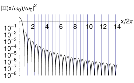
a)  b)

Figure 1. Sinusoidal transport. In a) a normalized transport function for a sine transport is shown with a transport in $2t_{0}=3$ time units. Figure b) shows the energy transfer as a function of $x/2\pi=t/T$, with $T=2\pi/\omega$ the period of the associated oscillation frequency. Zeros occur at the positions $x/2\pi=(2n+3)/4$ with $n=0,1,\ldots$. See text for details.

The energy transfer is decaying overall, but shows some oscillations arising from the dependence on the energy transfer on the phase of the internal oscillation at $t_{0}$. From Eq.(45) we see that for an extreme nonadiabatic transport, i.e. $x\sim 0$, we have gained the full potential energy of $m\omega_{0}^{2}b^{2}/2$. Depending on the exact transport duration we observe regular intervals where the energy drops to zero and no energy remains in the internal oscillator’s motion after the interval length $2t_{0}$. This is due to the phase sensitivity of the transport. From Eq.(46) we have the proportionality $|\tilde{\Xi}|^{2}\propto(1+\cos(2x))$, so that we expect the first zero for $x/2\pi=1/4$. However, for a transport in a harmonic well we need at least half an oscillation period for the ion to move to the other turning point, therefore we have instead $x/2\pi=3/4$ which is seen in Fig.1b) as the first root of the adiabatic factor. The denominator in Eq.(46) cancels the first root. The adiabatic energy transfer corresponds to the envelope of this function and is given by $4/(1-\left(2x/\pi\right)^{2})^{2}$. As we will see in the following the decay of the envelope can be sped up for different choices of the transport function.

Typically, we want to have $mb^{2}\omega_{0}|\tilde{\Xi}/\omega_{0}|^{2}/8\hbar\lesssim 1$ in order to limit the maximum transferred energy to a few vibrational quanta. Let us consider some typical parameters for traps currently in use; we choose the axial frequency $\omega=2\pi\cdot 3~{}\text{MHz}$, a typical average transport distance of about four traps (=control electrode widths), i.e. $b=400~{}\mu m$, and $m=9.01218~{}u$ equal to the mass of a Beryllium ion. Then the adiabatic suppression factor should obey

$$|\Xi/\omega_{0}|^{2}<2\cdot 10^{-8}.$$ (47)

In Fig.1b) we have not plotted the whole range until this criterion is fulfilled. It is satisfied for about $x/2\pi\gtrsim 30$. Thus, for the given case adiabatic transport happens on a rather long time scale, i.e. durations of $2\cdot x/2\pi=2t_{0}/T=60$ cycles. The transport in the experiment [18] which has used this transport function was performed over three times this distance requiring that $|\Xi/\omega_{0}|^{2}$ is lower by a factor of $9$ more. The adiabatic envelope has decayed to this value at about $x/2\pi\sim 52$ yielding a transport duration of $2t_{0}/T=104$ cycles. Using a sine transport function the experimentally measured limit was around $2t_{0}/T=157$ oscillation cycles (where $2t_{0}=54~{}\mu s$ and $\omega_{0}=2\pi~{}2.9~{}\text{MHz}$). This appears reasonable because the electrode array that was used in [18] was rather sparse, thus not allowing for full control and maintaining the conditions assumed in this paragraph properly. Also, the envelope in this region is quite flat; so within the uncertainties of the experiment, the experimentally observed limit is in reasonable agreement with our estimation.

We will look at an error function transport which turns out to be advantageous to the sine function in the second example

$$\tilde{q}_{0}(s)=\text{Erf}(2s/t_{p})/\text{Erf}(2t_{0}/t_{p})\qquad\text{for}\qquad-t_{0}<s<t_{0},$$ (48)

where we renormalized it to arrive at the times $\pm t_{0}$ at the start and end position. In addition we have introduced another time $t_{p}$ which is nearly reciprocal to the slope of the transport function at the central point $t=0$. Fig.2a) is a graph of this function for $(t_{p}=1,t_{0}=3/2)$ in arbitrary time units.

a)  b)

Figure 2. Error function transport. a) graph of the renormalized error function. b) Adiabatic suppression factor for the error function transport. Details are given in the text.

Since we truncate the error function, we violate the second initial condition in Eq.(2) in a strict sense. However, we are interested only in settings where $t_{p}/2t_{0}<1$, so that this constraint for the velocity can be satisfied arbitrarily well. The adiabatic suppression factor can be evaluated analytically

$$\tilde{\Xi}(x/\omega_{0})/\omega_{0} \sim 2e^{-y^{2}/16}\text{Re}\left\{\text{Erf}\left[2x/y+iy/4\right]\right\}/\text{Erf}\left[2x/y\right]\quad\times\text{phase factor}$$ (49)

$$\stackrel{{\scriptstyle 2x/y\rightarrow\infty}}{{\longrightarrow}}2e^{-y^{2}/16}\quad\times\text{phase factor},$$

neglecting the part resulting from the finite initial and final velocities, and using the dimensionless variable $y=\omega_{0}t_{p}$. Fig.2b) illustrates the situation for $y=12$ and $x/2\pi$ in a range of time intervals the same as for the sine transport but also satisfying $2t_{0}/t_{p}>1$. It is clear that by using the error function the transport can be performed much faster than with a sine transport function, while still satisfying inequality Eq.(47). The full transport can now be performed in $2x/2\pi\sim 6$ cycles with tolerable energy transfer. Interestingly, taking the limit for large $2x/y$ ratios in Eq.(49) removes the phase-sensitivity completely. However, we also want to note that the differences observed in these examples depend on experimental circumstances, e.g. for very short transport distances, the adiabatic suppression factor does not have to be small. In this case the differences between the adiabatic suppression factors is marginal in a qualitative sense. This can be seen in comparing Fig.1b) and Fig.2b) for cases when only about $|\Xi/\omega_{0}|^{2}<10^{-3}$ is required, e.g. occuring for transport distances much less than an electrode width. On the other hand we find an interesting and advantageous distance scaling behaviour from Eq.(49): transporting longer distances does not require much longer time intervals. For example, Steane [20] estimated that within large-scale operation for the processing of a typical gate an average transport distance of $\sim 22$ traps is needed. By employing an error function transport we find that this is feasible with less than a quantum of transferred energy using the parameters $(y=13,x/2\pi=4)$, i.e. in already about 8 oscillation cycles, only about a third more time than for a transport over $4$ traps. The average velocity for such a transport is then considerably higher.

6.2. Near-optimum transport functions

In an attempt to optimize the transport function we can expand expression Eq.(49) up to the first order correction [31]

$$\tilde{\Xi}(x/\omega_{0})_{y}\stackrel{{\scriptstyle r\rightarrow\infty}}{{\sim}}2\omega_{0}\left(e^{-b^{2}}-\frac{e^{-r^{2}}}{\sqrt{\pi}\sqrt{r^{2}+b^{2}}}\ \cos(2rb+\arctan(b/r))\right)/\text{Erf}\left[r\right]~{}\times\text{phase factor},$$ (50)

with $r=2x/y\equiv 2t_{0}/t_{p}$, $b=y/4$. Because of $2rb=x$ the zeros of the suppression factor $|\Xi|^{2}$ are equally spaced as in the sinusoidal example if we disregard the phase in the cosine function, i.e. half periods $\Delta(x/2\pi)=1/2$ since the particle can arrive from two different turning points at the end of the transport. From this expansion it is clear that the ratio $r$ basically determines the magnitude of the second term on the rhs of Eq.(50) and suppresses the phase sensitivity as it increases. If $r$ is chosen large enough the energy transfer is dominated by $b$. To find some conditions that are close to optimum we proceed in the following way: first, from the transport distance and achievable frequency we can evaluate the upper bound for the adiabatic suppression factor as in Eq.(47). Because we have to satisfy $2t_{0}>t_{p}$ we then choose $b$ large enough to suppress the first exponential factor to fulfill the given criterion. This procedure defines the asymptotic value of energy transfer for large $x/2\pi$ as shown in Fig.2b). We then choose the interval length $x/2\pi=rb/\pi$ by defining $r$ such that we are just in the asymptotic range. The near phase-insensitivity can then be thought of as a result of the extremely slow start where the phase information in the limiting case $r\rightarrow\infty$ in Eq.(49) gets totally lost.

6.3. High-frequency limit, adiabatic transport, and approximate trajectories

To better understand the behaviour discussed in previous sections, we present a few more general considerations. We write the time-dependence of the transport function according to $q_{0}(t)=\vartheta_{0}(t/t_{0})=\vartheta_{0}(\tau)$ so that $\vartheta_{0}$ only depends on the dimensionless variable $\tau$ (for the error function example we also keep the ratio $t_{p}/t_{0}$ fixed). Making the substitution $t^{\prime}\rightarrow\tau$ in the integral in Eq.(43) we find

$$\Xi(t_{0})/\omega_{0} =(\omega_{0}t_{0})^{-1}\int_{-1}^{1}d\tau\ e^{-i\omega_{0}t_{0}\cdot\tau}\vartheta^{\prime\prime}_{0}(\tau)\quad\times\text{phase factor}$$ (51)

$$\stackrel{{\scriptstyle\omega_{0}t_{0}\rightarrow\infty}}{{\sim}}2\cdot\sum_{n=0}^{N}\frac{\vartheta_{0}^{(n+2)}(-1)}{(-\omega_{0}t_{0})^{n+2}}~{}\cos(\omega_{0}t_{0}+n\pi/2)\quad\times\text{phase factor}.$$

The exponent in the integral relates the two time scales in $\omega_{0}$ and $t_{0}$. Using the method outlined in appendix A we expand it into the sum given in the second line in the limit $\omega_{0}t_{0}\rightarrow\infty$ assuming that $\vartheta_{0}$ is sufficiently smooth. In this expansion the derivatives at the start position (and end position due to anti-symmetry) define the energy transfer in the transport, and thus fully characterize the transport function for the transferred energy in the adiabatic limit. This provides us with a reason for the difference we observed above for the error function and sine examples. The second derivative for the sinusoidal transport is nonzero at $\pm t_{0}$ and much larger than in the case of the error function. In the latter all derivatives are damped by a gaussian while the ones for the sine transport alternate. Furthermore, we see that we can in general decrease the transferred energy for larger values of the product $\omega_{0}t_{0}$, i.e. by taking $\omega_{0}$ to inifinity (high-frequency limit), we can lower the adiabatic suppression arbitrarily, on the other hand, slowing down the motion by increasing the length of the duration of the transport $2t_{0}$, we move into the adiabatic regime. For infinitely slow motion we end up with zero transferred energy. These two limiting cases are formally equivalent because the energy transfer depends only on their relative time scale. We can perform the same expansion starting from Eq.(43) directly and use the relation $u_{c}(t)=[\Xi(t)-\Xi^{*}(t)]/2i\omega_{0}$ to find approximate trajectories valid in the same limits

$$u_{c}(t) =-\sum_{n=0}^{N}\frac{1}{\omega_{0}^{n+2}}\left[\cos\left(\dfrac{n\pi}{2}\right)q^{(n+2)}_{0}(t)-\cos\left(\omega_{0}(t+t_{0})-\dfrac{n\pi}{2}\right)q^{(n+2)}_{0}(-t_{0})\right].$$

7. Regularized trap-electrode waveforms, potential fluctuations and aspect-ratio rule

7.1. Determination of waveforms

So far, we have said nothing about how to determine the waveforms applied to the electrodes. As soon as we have the waveforms at hand for a given model electrode configuration we can determine the magnitudes of perturbations. This is done in the next section. Here, we seek optimum solutions for a given electrode structure in order to keep the uncontrolled part $\phi_{\text{res}}(q)$ of the total potential in Eq.(4) small. The time-dependent electric potential is created by a linear superposition of the available control potentials $\phi_{m}(q)$ and dimensionless time-dependent amplitudes $a_{m}(t)$ of the form

$$\phi(q,t)=\sum_{m}a_{m}(t)\phi_{m}(q).$$ (52)

To optimize waveforms for the time-dependent amplitudes for the transport problem we find a measure of the discrepancy by integrating over the residual non-matched part according to

$$\min_{a_{m},\varphi_{0}}\int_{q_{0}(t)-\delta q}^{q_{0}(t)+\delta q}\left|\phi_{\text{res}}(q,t)\right|^{2}dq\qquad\forall~{}t$$ (53)

while $\phi(q,t)$ from Eq.(52) enters here through Eq.(4). For any time $t$ we want to find a set $a_{m},\varphi_{0}$ for which expression Eq.(53) is minimal. The integration is performed over an interval moving with the minimum of the parabolic potential well, i.e. $[q_{0}(t)-\delta q,q_{0}(t)+\delta q]$ and assuming a unity weight factor in the integrand. We do not consider in this range any lag of the ion due to acceleration and deceleration since for an adiabatic transport and experimental conditions the lag is much smaller compared to the optimization range. $\varphi_{0}(t)$ represents here another degree of freedom that does not perturb the dynamics but might allow one to more optimally choose the harmonic potential well by arbitrarily offsetting the desired parabolic potential for best fit. Condition Eq.(53) is readily converted into a linear system of equations by taking partial derivatives for the amplitudes $a_{m}$ and $\varphi_{0}$, and setting them all equal to zero. The minimization problem in Eq.(53) then reads

$$\sum_{m=1}^{n_{\text{el}}}a_{m}(t)\underbrace{\int dq\ \phi_{m}\phi_{j}}_{{\bf S}_{a}}+\varphi_{0}(t)\underbrace{\int dq\ \phi_{j}}_{\underline{S}_{\varphi_{0}}}=\frac{m\omega^{2}}{2Q}\underbrace{\int dq\ (q-q_{0}(t))^{2}\phi_{j}}_{\underline{K}}\quad\forall~{}j,$$ (54)

where we dropped the explicit integral bounds and arguments of the potentials $\phi_{m}(q)$ for the sake of simplicity. Bold symbols denote matrices, underlined symbols vectors.

The optimization problem can then be formulated in terms of the linear system

$${\bf S}_{+0}\cdot\underline{a}_{+0}\equiv\left(\begin{array}[]{cc}{\bf S}_{a}&\underline{S}_{\varphi_{0}}\end{array}\right)\cdot\left(\begin{array}[]{c}\underline{a}\\ \varphi_{0}\end{array}\right)=\eta\underline{K}\quad\forall t,$$ (55)

with $\eta=m\omega^{2}/2Q$. All quantities are functionals of $q_{0}$ and for a given transport function $q_{0}(t)$, we need to solve the equations at every point in time. As a result we obtain the waveforms $a_{m}(t)\equiv a_{m}[q_{0}(t)]$.

Typically we choose an optimization range of $2\delta q\sim 0.5W$ for electrodes of width $W$. This is usually much smaller than the mean distance between most of the contributing electrodes to the center of the parabolic well. Thus, due to the slow decay of the axial potentials, the curvatures of distant electrodes are similar, and their contribution differs locally only by a multiplication constant. This is particularly true for experimental situations where the high electrode density typically makes the system Eq.(55) nearly singular. A straightforward least-square method, such as

$$\underline{a}_{+0}=\text{arg}\min_{\underline{a},\varphi_{0}}\left\{\|{\bf S}_{+0}\cdot\underline{a}_{+0}-\eta\underline{K}\|^{2}\right\},$$ (56)

is therefore not well suited for finding waveform amplitudes. For high electrode density, a tiny step $q_{0}\rightarrow q_{0}+\delta$ might change the individual electrode amplitudes exponentially fast. In these cases the matrix ${\bf S}_{+0}$ in Eq.(55) filters out too much information from $\underline{a}_{+0}$ to invert this system properly. In mathematical language these kind of problems belong to the family of discrete ill-posed problems that can be numerically solved using regularization approaches [35]. Here, the lost information is fed back in the minimization process via a Lagrangian multiplier concerning the smoothness of $a_{m}(t)$, or curvature etc. in amplitude space. If we apply a Tikhonov regularization to the given problem we have to solve

$$\underline{a}_{+0,\nu}=\text{arg}\min_{\underline{a},\varphi_{0}}\left\{\|{\bf S}_{+0}\cdot\underline{a}_{+0}-\eta\underline{K}\|^{2}+\nu^{2}\|{\bf L}(\underline{a}_{+0}-\underline{a}_{+0}^{*})\|^{2}\right\}$$ (57)

in order to determine smooth time-dependent waveform amplitudes $a_{m}(t)$. In Eq.(57) the regularization parameter $\nu$ corresponds to a weight factor between the original least-square minimization and the additional side constraints, while $\underline{a}_{+0}^{*}$ can be used to find solutions near a prescribed setting. The smoothing properties of this optimization originate from a common and simultaneous minimization of both terms. $L$ is a linear operator that can be used to feed back different kinds of information to the amplitudes. For the results given here we took for $L$ the unity operator, and also $\underline{a}_{+0}^{*}=0$. Since we only want to limit the amplitudes $a_{m}$ to some appropriate experimental values and stabilize the solution, our interest is not to determine the overall minimum of Eq.(57) in a self-consistent way. For our convenience we choose $\nu$ manually to make the parameters compatible with available technology.

We can summarize the advantages of these methods to the current optimization problem:

1. The regularization method selects only nearby electrodes for creating a local parabolic potential, and disregards tiny linear contributions from distant electrodes which would require large amplitudes to effect small changes.

2. The choice of the regularization parameter limits the amplitudes $a_{m}$ to practical experimental values.

3. It is robust against changing the electrode density (here, governed by the widths W). This will be of importance in the next section.

4. It stabilizes the output waveforms and smoothes sharp features in the time-dependence of the amplitudes. Different constraints can be set via the $L$ operator, defining bounds or curvatures in the amplitude space.

For more detailed information we refer the reader to the mathematical literature [35]. A typical example of a parabolic potential created through superposition of an array of electrodes and the time-dependence of amplitudes is shown in Fig.4 and further discussed in the next section.

7.2. Potential fluctuations and aspect-ratio rule

Based on a reasonable multi-electrode structure we want to estimate how well we can meet the requirements on transport potentials stated above, in particular, how stringently we can meet $|a^{\prime}_{\text{res}}(q_{0})|/\omega_{0}^{2}\ll 1$ and $|a_{\text{res}}(q_{0})|\ll|\ddot{q}_{0}|$. We employ the definition of waveforms and the method from the previous section for extracting the residual, uncontrolled potential $\phi_{\text{res}}$ from which we perturbatively derive the effect of imperfections on the transport. As a simple model electrode structure for transport in single and multi-layer traps, we use the “railway track“ electrode configuration sketched in Fig.3a) which might be a simple model for transport in single and multi-layer traps [19, 22, 32, 33]. The transport occurs along the long arrow where we assume the ion is held radially by RF fields and controlled axially by the electrical fields arising from the potentials of the “stripe“ electrodes depicted in Fig.3a). We are mainly interested in the scaling behaviour as a guideline for general design rules. Waveforms that are actually used in experiments should be based on more accurate numerical potentials and generalized versions of Eq.(54) for all three dimensions. We are finally interested in the trade off between adding electrodes, by shrinking the electrode distances/widths along x, and the amount of control that is gained in that way.

We can model this arrangement as a sum over the potentials $\phi_{m}(x)$ of several infinitely long (in the y-direction) stripe electrodes that are distributed along the x-axis

$$\phi(\hat{x})=\sum_{m}a_{m}\phi_{m}(\hat{x})=\frac{1V}{\pi}\sum_{m}a_{m}\arctan\left(\frac{\hat{W}}{1+(\hat{x}-m\hat{W})^{2}-\hat{W}^{2}/4}\right),$$ (58)

where each $\phi_{m}(x)$ is the exact solution of the Poisson equation for an infinitely long stripe at position $m\cdot W$ that is embedded in a ground plane. For convenience we choose for the individual potentials in this basis set a potential on the electrodes of $1\text{Volt}=1~{}V$. We denote symbols with a hat as quantities normalized to the ion distance $z_{\text{ion}}$ to the surface, e.g. the normalized electrode width $\hat{W}=W/z_{\text{ion}}$. Fig.3b) shows the behaviour of $\phi_{0}(\hat{x})$ for various geometric aspect ratios $\hat{W}$. We see that a plateau-like structure starts to form for $\hat{W}\sim 2$ and larger resulting in small field gradients along the transport direction in the center of each stripe electrode. The maximum frequency at the center of electrode $m=0$ is obtained from

$$\omega^{2}(\hat{W},z_{\text{ion}})=\left.\frac{Q}{mz_{\text{ion}}^{2}}\frac{\partial^{2}}{\partial\hat{x}^{2}}\phi_{0}(\hat{x})\right|_{\hat{x}=0}=-\frac{2a_{0}}{\pi m}\frac{1eV}{z_{\text{ion}}^{2}}\frac{\hat{W}}{(\hat{W}/2)^{4}+3\hat{W}^{2}/2+1}.$$ (59)

The proportionality $\omega\propto z_{\text{ion}}^{-1}$ is rather unusual and stems from the fact that we scale only a single dimension (along $x$). The last factor of the second equation is solely defined by the aspect ratio $\hat{W}$ and thus by the geometry of the trap. It exhibits a maximum for $\hat{W}\sim 0.78$ and decreases only significantly for small width-distance ratios $\hat{W}<0.5$. Using the mass of Beryllium, $\hat{W}=1$, amplitude $a_{0}=-2$ and $z_{\text{ion}}=40~{}\mu m$ as the ion surface distance for the surface-electrode trap as used in [32], we find an axial frequency of about $\omega_{0}\sim 2\pi\cdot 9~{}\text{MHz}$. We chose this low value for $|a_{0}|$ to be compatible with typical maximum voltages as created by CMOS electronics [19]. With these parameters we have created waveforms for the transport of a confining harmonic well utilizing the regularization approach of the last section. We used a set of $41$ electrodes while the transport was over four electrode widths, $\hat{b}=4$, around the central electrode $21$ of this array. For the transport we used the error function Eq.(48) of Sect.6 with a transport duration of $8$ oscillation cycles $x/2\pi=4$ and $y=12$. We then determined the lowest order deviations from an ideal harmonic potential with constant trap frequency and controlled acceleration, $\omega(t)/\omega_{0}$ and $-a_{\text{res}}(q_{0})/\omega_{0}^{2}$, respectively, in Eq.(6) for the aspect-ratios $\hat{W}=(0.5,1.0,1.5,2.0)$. Figs.4a) and b) illustrate an example for the superposed potentials, and for a set of waveform amplitudes for an error function transport in $8$ oscillation cycles.

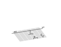
a)  b)

Figure 3. a) The control electrode array model discussed in the text with $x$ the axial coordinate, $z_{\text{ion}}$ the vertical distance of trapped ions to the electrode plane, and $W$ width of an electrode. No RF electrodes are shown to hold the ion in radial directions. The electrode ’stripes’ are assumed infinitely extended along $\pm y$, and arbitrarily many along $\pm x$. Ions are transported along the long arrow from $-b/2$ to $+b/2$. b) Modulus of the electric potential of a single electrode at height $z_{\text{ion}}$ along x (relative to the center of that electrode and normalized to $z_{\text{ion}}$). The electrode is embedded in an infinite ground plane and held at $-1~{}V$, and $\hat{W}=W/z_{\text{ion}}.$

The choice of the regularization parameter $\nu$ is not obvious, because we have to deal with a set of near-singular matrices all at once. As mentioned earlier we do not aim for self-consistent methods to determine $\nu$ and an absolute minimum of the expression Eq.(57) [35]. In our context we are more interested in a feasible implementation compatible with given experimental constraints. The choice of the regularization parameter affects both the stability of the linear system and the size and smoothness of the amplitude vector $a_{m}$. In a strongly regularized inversion more stability is added to the solution, forcing the amplitudes to be of limited size. Because of this bound the solution can not closely approximate the desired shape of the potential anymore, so the deviations from the ideal case increase. A weak regularization scheme, on the other hand, adapts more closely to the desired potential shape, but reveals random fluctuations and noise on the solution waveforms $a_{m}(t)$. Also the singular behaviour increases dramatically with an increase of the number of electrodes, and larger parameters $\nu$ have to be chosen. This latter property makes a direct comparison of the results among various aspect-ratios $\hat{W}$ difficult. Nevertheless, we can make some qualitative and general statements.

The results for our sample configuration are summarized in Fig.5. The upper graph in Fig.5 displays the uncontrolled acceleration $-a_{\text{res}}(q_{0})/\omega_{0}^{2}$, and the middle and lower graphs the frequency modulation $\omega(t)$ for various aspect ratios. In both figures a dramatic change of the curves is observed around $\hat{W}\sim 1$. While for smaller ratios the frequency fluctuations are in the percentage range (middle panel), the emulation of the potential for larger ratios is much worse due to the constraint $|a_{m}|\leq 2$ (lower panel). Frequencies drop by more than $90\%$ already for the $\hat{W}=2$ calculation. Only in the strongly regularized scheme, did we find a direct correlation of the solution vector $a_{m}$ to the choice of the regularization parameter. In the weakly regularized scheme the amplitudes were limited by other lower bounds, and the waveform solution appeared similar over a large range of $\nu$, but exhibited a much noisier behaviour. This enhanced sensitivity is an indication that inclusion of more electrodes (smaller $\hat{W}$) does not improve the quality of the solution anymore. The linear system becomes more singular and exhibits more rank-deficiency, i.e. rows and columns become more equal and their inclusion adds more redundancy. For the given parameters we observed that for $\hat{W}=0.5$ the transition from a regularized to a weakly regularized solution occured. Therefore, our results indicate that $\hat{W}=0.5-1.0$ should be optimal for the configuration discussed here. For larger aspect- ratios we found that the coverage of curvatures of the individual potentials along the transport axis is not sufficient for the necessary amount of control.

The other constraint, i.e. $|\hat{a}_{\text{res}}(q_{0})|\ll|\ddot{\hat{q}}_{0}|$, of a controlled transport force, has to be interpreted dynamically. Since the acceleration force depends on the time duration in which the transport is performed, this requirement can be violated for a slower transport. In Fig.5) we show that in the initial phase the perturbations overwhelm the transporting acceleration for aspect ratios $\hat{W}\geq 1.5$ or larger. Results for smaller aspect ratios are not given in this figure because the transport force by far dominates the excess force and lead to a fully controlled transport.

In general, fluctuations in the frequency and transport force affect an energy transfer according to Eq.(23). This introduces violations to the symmetry of the transporting force and leads to an enhanced energy transfer as seen from Eq.(44). We have not included higher order terms in our discussion, because we aim for experimental conditions to perform a transport in the well-controlled regime. However, they are inevitable for longer transport distances and other types of motion, such as nonadiabatic transport, or splitting of ion groups where they might lead to large energy transfers.

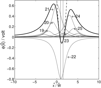
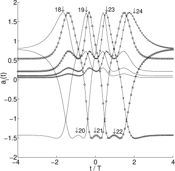
a)              b)

Figure 4. a) Creation of a harmonic well by superposing potentials of the electrodes of the stripe configuration of Fig.3a). The fine lines represent individual electrode potentials that sum up to the total potential represented by the thicker line. The dashed-dotted line shows the ideal harmonic potential and the two vertical lines indicate the range of optimization at this given location. By symmetry the extrema of the individual electrode potentials are located at integer values of $\hat{x}/\hat{W}$, with the maximum of electrode potential 21 at the origin. b) Waveform amplitudes of electrodes 18 to 24 for a transport from trap 19 to 23 for $\hat{W}=1$. Waveforms from more distant electrodes still contribute but are not shown for the sake of clarity. Amplitudes 21-24 are marked by symbols for better visualizing their traces. The transport is done according to an error function, while the abscissa represents time in units of oscillation periods $t/T$.

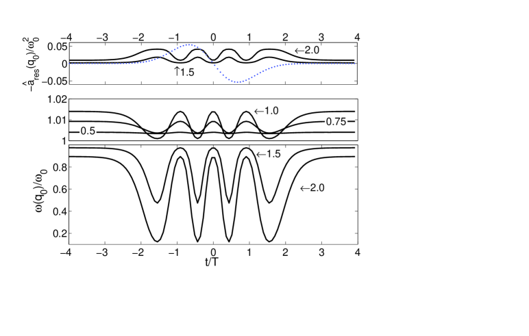
Figure 5. First and second order perturbation to the transport (thick lines), and their dependence on various aspect ratios $\hat{W}$. The abscissa $t/T$ corresponds to the number of oscillation cycles with period $T=2\pi/\omega_{0}$. The labels on the graphs denote the value of $\hat{W}$. (Upper panel) Residual, uncontrolled acceleration $-\hat{a}_{\text{res}}(q_{0})/\omega_{0}^{2}$ (dimensionless) which should be compared to $\ddot{\hat{q}}_{0}/\omega_{0}^{2}$ (dotted line). This is only given for the large aspect ratios $\hat{W}=1.5,2.0$. The graphs for smaller ratios would be close to zero on this scale. (Middle and lower panels) Relative frequency modulation $\omega(q_{0})/\omega_{0}$ during an error function transport for various aspect ratios. For explanations see text.

8. Conclusions

In conclusion, we have analyzed the dynamics of single ion transport in microstructured linear Paul trap arrays. We have modeled the transport by a forced and parametrically excited harmonic oscillator and have presented a theoretical framework for its description. We have derived exact analytical expressions for the classical as well as quantum dynamics and reviewed their related properties. In particular we have expressed the Heisenberg operators by the approach of Kim et al. [21] through the dynamical quantities of the related classical solution. We have given explicit analytical expressions for the classical energy transfer involved in these transport phenomena and derived expressions for the lowest order deviations from ideal transport that will necessarily appear for unfavourable ion trap layouts. For current trap technology we have evaluated durations for a fast adiabatic transport and found that they depend strongly on the external force employed in the transport. According to these results, the adiabatic single ion transports of reference [18] could be sped up by more than an order of magnitude with negligible energy transer to the motion. We determined appropriate transport waveforms and found that with an adiabatic transport over four electrode stripes of size roughly equal to the distance of the ion to the nearest electrode and frequencies in the range of $\sim 9~{}\text{MHz}$ is feasible in about 6 oscillation cycles. Our results also indicate that a full control over the transport is available, where perturbations to a harmonic oscillator potential are negligible at all positions and times. By directly relating deviations from these ideal potentials to the aspect ratio of the trap, we have found a practical design rule that should be valid for trap layouts more general than the one given here. The ratio of a control electrode width to the distance to the ion should be in the range $0.5-1$ for a well-controlled regime. Our example suggests that a higher electrode density does not appreciably improve transport performances. This provides important insight into the amount of resources needed to realize large scale implementations of ion trap based quantum computers. Transport in a confining well of constant frequency might also enable continuous cooling processes during the transport. If eventually experiments allow one to maintain a well-controlled regime during the transport, performing quantum processing during transport is conceivable, possibly leading to appreciably shorter processing times.

9. Acknowledgements

R.R. acknowledges support by the Alexander von Humboldt Foundation during the course of this work. Work also supported by DTO and NIST. We thank A. Steane, T. Rosenband and J. Wesenberg for helpful comments on the manuscript.

Appendix A Integral expansion

We employ a mathematical theorem proven within the formalism of h-transforms, see for example theorem 3.2 of [36]: If $g(\tau)$ has $N+1$ continuous derivatives while $g^{(N+2)}$ is piecewise continuous on the real axis $[a,b]$ then

$$I(\lambda)=\int_{a}^{b}e^{-i\lambda\tau}g(\tau)d\tau\stackrel{{\scriptstyle\lambda\rightarrow\infty}}{{\sim}}\sum_{n=0}^{N}\frac{(-1)^{n}}{(-i\lambda)^{n+1}}\left[g^{(n)}(b)e^{-i\lambda b}-g^{(n)}(a)e^{-i\lambda a}\right].$$ (60)

If we also require $\lim_{\tau\rightarrow a+}g^{(n)}(\tau)=\lim_{\tau\rightarrow b-}g^{(n)}(\tau)=0$ for $n=0,..,N-1$ it holds that $I(\lambda)=o(\lambda^{-N})$.

References

- [1] D.J. Wineland, C. Monroe, W.M. Itano, D. Leibfried, B.E. King, and D.M. Meekhof, J. Res. Natl. Inst. Stand. Technol. 103, 259 (1998)
- [2] D. Kielpinski, C. Monroe, D. J. Wineland, Nature 417, 709 (2002)
- [3] Nielsen, M. A. and Chuang, I. L Quantum Computation and Quantum Information (Cambridge Univ. Press, Cambridge, 2000).
- [4] Cirac, J. I., Zoller, P., Phys. Rev. Lett. 74, 4091 (1995)
- [5] D. Leibfried, E. Knill, S. Seidelin, J. Britton, R. B. Blakestad, J. Chiaverini, D. B. Hume, W. M. Itano, J. D. Jost, C. Langer, R. Ozeri, R. Reichle, D. J. Wineland, Nature 438, 639 (2005)
- [6] H. Häffner, W. Hänsel, C. F. Roos, J. Benhelm, D. Chek-al-kar, M. Chwalla, T. Körber, U. D. Rapol, M. Riebe, P. O. Schmidt, C. Becher, O. Gühne, W. Dür, and R. Blatt, Nature 438, 643 (2005)
- [7] D. Leibfried, B. DeMarco, V. Meyer, D. Lucas, M. Barrett, J. Britton, W. M. Itano, B. Jelenkovic, C. Langer, T. Rosenband and D. J. Wineland, Nature 422, 412 (2003)
- [8] C. Langer, R. Ozeri, J. D. Jost, J. Chiaverini, B. DeMarco, A. Ben-Kish, R. B. Blakestad, J. Britton, D. B. Hume, W. M. Itano, D. Leibfried, R. Reichle, T. Rosenband, T. Schaetz, P. O. Schmidt, D. J. Wineland, Phys. Rev. Lett. 95, 060502 (2005)
- [9] H. Häffner, F. Schmidt-Kaler, W. Hänsel, C.F. Roos, T. Körber, M. Chwalla, M. Riebe, J. Benhelm, U. D. Rapol, C. Becher, R. Blatt, Appl. Phys. B 81, 151 (2005)
- [10] P. C. Haljan, P. J. Lee, K-A. Brickman, M. Acton, L. Deslauriers, and C. Monroe, Phys. Rev. A 72, 062316 (2005)
- [11] M. J. McDonnell, J.-P. Stacey, S. C. Webster, J. P. Home, A. Ramos, D. M. Lucas, D. N. Stacey, and A. M. Steane, Phys. Rev. Lett. 93, 153601 (2004)
- [12] DiVincenzo, D. P., Fortschr. Phys. 48, 771 (2000)
- [13] M. Riebe, H. Häffner, C. F. Roos, W. Hänsel, J. Benhelm, G. P. T. Lancaster, T. W. Körber, C. Becher, F. Schmidt-Kaler, D. F. V. James, and R. Blatt, Nature 429, 734 (2004).
- [14] M. D. Barrett, J. Chiaverini, T. Schaetz, J. Britton, W. M. Itano, J. D. Jost, E. Knill, C. Langer, D. Leibfried, R. Ozeri, D. J. Wineland, Nature 429, 737 (2004)
- [15] J. Chiaverini, D. Leibfried, T. Schaetz, M. D. Barrett, R. B. Blakestad, J. Britton, W. M. Itano, J. D. Jost, E. Knill, C. Langer, R. Ozeri, D. J. Wineland, Nature 432, 602 (2004)
- [16] J. Chiaverini, J. Britton, D. Leibfried, E. Knill, M. D. Barrett, R. B. Blakestad, W. M. Itano, J. D. Jost, C. Langer, R. Ozeri, T. Schaetz, D. J. Wineland, Science 308, 997 (2005)
- [17] K.-A. Brickman, P. C. Haljan, P. J. Lee, M. Acton, L. Deslauriers, and C. Monroe, Phys. Rev. A 72, 050306(R) (2005)
- [18] M. A. Rowe, A. Ben-Kish, B. DeMarco, D. Leibfried, V. Meyer, J. Beall, J. Britton, J. Hughes, W. M. Itano, B. Jelenkovic, C. Langer, T. Rosenband, D. J. Wineland, Quant. Inf. Comput. 4, 257 (2002)
- [19] J. Kim, S. Pau, Z. Ma, H. R. McLellan, J. V. Gates, A. Kornblit, R. E. Slusher, R. M. Jopson, I. Kang, and M. Dinu, Quant. Inf. Comp. 5, 515 (2005).
- [20] A. Steane, quant-ph/0412165
- [21] Hyeong-Chan Kim, Min-Ho Lee, Jeong-Young Ji, Jae Kwan Kim, Phys.Rev. A, 53, 3767, (1996)
- [22] D. Stick, W. K. Hensinger, S. Olmschenk, M. J. Madsen, K. Schwab and C. Monroe, Nature Physics 2, 36-39 (2006)
- [23] W. K. Hensinger, S. Olmschenk, D. Stick, D. Hucul, M. Yeo, M. Acton, L. Deslauriers, C. Monroe, and J. Rabchuk, App. Phys. Lett. 88, 034101 (2006).
- [24] Jeong-Young Ji, Jae Kwan Kim, Sang Pyo Kim, Phys.Rev. A, 51, 4268, (1995)
- [25] Jeong-Young Ji, Jae Kwan Kim, Phys.Rev. A, 53, 703, (1996)
- [26] D.J. Wineland et al. , Proc. 2005 ICOLS conf., available at http://tf.nist.gov/timefreq/general/pdf/2078.pdf
- [27] K. Husimi, Prog. Theor. Phys., 9, 381, (1953)
- [28] E. H. Kerner, Can. J. Phys., 36, 371, (1958) Quantum Physics, Dover Publications, Inc., New York
- [29] R. M. Kulsrud, Phys. Rev. 106, 205 (1957)
- [30] H. R. Lewis, J. Math. Phys. 9, 1976 (1968)
- [31] H.O. Di Rocco, M. Aguirre Tellez, Acta Physica Polonica A 106 (6), 817 (2004)
- [32] S. Seidelin, J. Chiaverini, R. Reichle, J. J. Bollinger, D. Leibfried, J. Britton, J. H. Wesenberg, R. B. Blakestad, R. J. Epstein, D. B. Hume, J. D. Jost, C. Langer, R. Ozeri, N. Shiga, D. J. Wineland, quant-ph/0601173
- [33] J. P. Home, and A. M. Steane, quant-ph/0411102.
- [34] L.D. Landau, E.M. Lifshitz, Mechanics, Third edition, Course of theoretical physics, Volume 1, Pergamon press, Oxford, UK, 1991.
- [35] P. C. Hansen, Rank-Deficient and Discrete Ill-Posed Problems: Numerical Aspects of Linear Inversion, SIAM, Philadelphia, 1998.
- [36] Bleistein, Norman and Handelsmann, Richard A. Asymptotic Expansions of Integrals, (Dover Publications, Inc. New York, 1986).