Casimir edge effects

Abstract

We compute Casimir forces in open geometries with edges, involving parallel as well as perpendicular semi-infinite plates. We focus on Casimir configurations which are governed by a unique dimensional scaling law with a universal coefficient. With the aid of worldline numerics, we determine this coefficient for various geometries for the case of scalar-field fluctuations with Dirichlet boundary conditions. Our results facilitate an estimate of the systematic error induced by the edges of finite plates, for instance, in a standard parallel-plate experiment. The Casimir edge effects for this case can be reformulated as an increase of the effective area of the configuration.

I Introduction

Casimir’s prediction for the force $F$ per unit area $A$ between two perfectly conducting infinite parallel plates at a distance $a$ Casimir:dh ,

$$\frac{F_{\|}}{A}=-2\gamma_{\|}\,\frac{\hbar c}{a^{4}},\quad\gamma_{\|}=\frac{\pi^{2}}{480}\simeq 2.056\times 10^{-2},$$ (1)

has a remarkable property: a straightforward dimensional analysis already fixes the powers of $\hbar$, $c$, and $a$ uniquely. In absence of any other dimensionful quantity, the effects of quantum fluctuations in this geometry can be summarized by a simple number: $2\gamma_{\|}$. This coefficient is universal in the sense that it does not depend on the microscopic details of the interactions between the fluctuating field and the constituents of the surfaces. It is completely fixed by specifying the geometry, the nature of the fluctuating field and the type of boundary conditions. For instance, for a fluctuating real scalar field with Dirichlet boundary conditions, the parallel-plate coefficient reduces exactly to $\gamma_{\|}$; the factor of 2 in Eq. (1) can be traced back to the two polarization modes of the electromagnetic field.

Away from the ideal Casimir limit, corrections to Eq. (1) arise from finite conductivity, surface roughness, thermal fluctuations and deviations from the ideal geometry. All these come with additional dimensionful scales, such as plasma frequency, length scales of roughness variation, temperature or surface-curvature radii. The corrections generically cannot be predicted from dimensional analysis, but its functional dependence on the further parameters has to be computed Klimtchiskaya:1999 ; Lambrecht:1999vd ; Sernelius ; Bezerra:2000 ; Bordag:2001qi ; Milton:2001yy ; Lambrecht:2005 .

The present work is devoted to an investigation of the Casimir force between disconnected rigid surfaces, which exhibits properties similar to Casimir’s classic parallel-plate configuration: unique dimensional scale dependencies and universal coefficients. The first property implies that the geometry is characterized by only one length scale, such as the distance parameter $a$. New Casimir configurations therefore necessarily involve edges, whose influence on the Casimir effect is an interesting and difficult question in itself. In view of the rapid progress in the fabrication and use of micro- and nano-scale mechanical devices accompanied by precision measurements of the Casimir forces in these systems Lamoreaux:1996wh ; Mohideen:1998iz ; Roy:1999dx ; Ederth:2000 ; Chan:2001 ; Chen:2002 ; Decca:2003td , a detailed understanding of Casimir edge effects is indispensable.

Straightforward computations of Casimir edge effects are conceptually complicated, since the fluctuation spectrum carries the relevant information in a subtle manner. A technique that facilitates Casimir computations from first field-theoretic principles is given by worldline numerics Gies:2001zp , combining the string-inspired approach to quantum field theory Schubert:2001he with Monte Carlo methods. As a main advantage, the worldline algorithm can be formulated for arbitrary Casimir geometries, resulting in a numerical estimate of the exact answer Gies:2003cv . Since the approach is based on Feynman path-integral techniques, the problem of determining the Casimir fluctuation spectrum is circumvented Gies:2005ym . The resulting algorithms are trivially scalable, and computational efforts increase only linearly with the parameters of the numerics.

Recent results obtained by worldline numerics Gies:2006bt go hand in hand with those obtained by new analytical methods Bulgac:2005ku ; Emig:2006uh ; Bordag:2006vc which are based on advanced scattering-theory techniques; excellent agreement has been found for the experimentally important sphere-plate and cylinder-plate Casimir configurations.

In the present work, we use worldline numerics to examine Casimir edge effects induced by a fluctuating scalar field, obeying Dirichlet boundary conditions (“Dirichlet scalar”). We compute Casimir interaction energies and forces between rigid surfaces. Our results can directly be applied to Casimir configurations in ultracold-gas systems Roberts:2005 where massless scalar fluctuations exist near the phase transition. For Casimir configurations probing the electromagnetic fluctuation field, the results for the universal coefficients may quantitatively differ, but our values can be used for an order-of-magnitude estimate of the error induced by edges of a finite configuration, thus providing an important ingredient for the data analysis of future experiments.

In addition to being a simple and reliable quantitative method, the worldline formalism also offers an intuitive picture of quantum-fluctuation phenomena. The fluctuations are mapped onto closed Gaußian random paths (worldlines) which represent the spacetime trajectories of virtual loop processes. The Casimir interaction energy between two surfaces can thus be obtained by identifying all worldlines that intersect both surfaces. These worldlines correspond to fluctuations that would violate the boundary conditions; their removal from the ensemble of all possible fluctuations thereby contributes to the (negative) Casimir interaction energy. The latter measures only that part of the energy that contributes to the force between rigid surfaces; possibly divergent self-energies of the single surfaces Graham:2002xq are already removed.

For a massless Dirichlet scalar, the worldline representation of the Casimir interaction energy reads Gies:2003cv ; Gies:2005ym

$$E=-\frac{1}{2}\frac{1}{(4\pi)^{2}}\int_{0}^{\infty}\frac{dT}{T^{3}}\,\left\langle\Theta_{\Sigma}[\mathbf{x}]\right\rangle_{\mathbf{x}}.$$ (2)

The expectation value in (2) has to be taken with respect to an ensemble of closed worldlines,

$$\langle\dots\rangle_{\mathbf{x}}:=\int_{\mathbf{x}(T)=\mathbf{x}(0)}\mathcal{D}\mathbf{x}\,\dots e^{-\frac{1}{4}\int_{0}^{T}d\tau{\dot{\mathbf{x}}}^{2}},$$ (3)

with implicit normalization $\langle 1\rangle_{\mathbf{x}}=1$. In Eq. (2), $\Theta_{\Sigma}[\mathbf{x}]=1$ if a worldline $\mathbf{x}$ intersects both surfaces $\Sigma=\Sigma_{1}+\Sigma_{2}$, and $\Theta_{\Sigma}[\mathbf{x}]=0$ otherwise. The worldline integral can also be evaluated locally, e.g., with the restriction to worldlines with a common center of mass, $\mathbf{x}_{\text{CM}}$, resulting in the interaction energy density $\varepsilon(\mathbf{x}_{\text{CM}})$, $E=\int d^{3}x\varepsilon(\mathbf{x}_{\text{CM}})$. The interaction energy serves as a potential for the Casimir force between rigid surfaces; the force is thus obtained by simple differentiation with respect to the distance parameters.

The worldline numerical algorithm corresponds to a Monte Carlo evaluation of the path integral of Eq. (3) with a discretized propertime $\tau$. In this work, we exploit the recent algorithmic developments detailed in Gies:2006cq .

II Casimir edge configurations

II.1 Perpendicular Plates

Let us first analyze a semi-infinite plate perpendicularly above an infinite plate at a minimal distance $a$, as first proposed in Gies:2005ym . This configuration is illustrated in Fig. 1 together with a worldline which contributes to the Casimir interaction energy, since it intersects both plates.

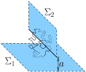
Figure 1: Sketch of the perpendicular-plates configuration. The minimal distance $a$ between the edge of the upper semi-infinite plate (thick solid line) and the lower infinite plate represents the only dimensionful length scale in the problem.

This configuration is translationally invariant only in the direction pointing along the edge with $a$ being the only dimensionful length scale. The Casimir force per unit length $L$ along the edge direction is thus unambiguously fixed by dimensional analysis,

$$\frac{F_{\bot}}{L}=-\gamma_{\bot}\,\frac{\hbar c}{a^{3}}.$$ (4)

Evaluating the worldline integral as outlined above, we obtain an estimate for the corresponding Casimir interaction energy density $\varepsilon(\mathbf{x})$, a contour plot of which is given in Fig. 2. For the universal coefficient, we obtain

$$\gamma_{\bot}=1.200(4)\times 10^{-2}.$$ (5)

The error is below the 1% level for a path ensemble of 40 000 loops with 200 000 points per loop (ppl) each. This coefficient is in agreement with the Casimir interaction energy computed in Gies:2005ym .

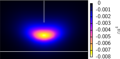
Figure 2: Contour plot of the Casimir interaction energy density $\varepsilon$ for the perpendicular-plate configuration. The white lines mark the position of the plates to guide the eye. Ensemble parameters: 2000 loops with 10 000 ppl.

II.2 Semi-infinite plate parallel to an infinite plate

Next we consider a first variant of the parallel-plate configuration, where one of the plates is only semi-infinite with an edge on one side; see Fig. 3. This configuration can be viewed as an idealized limit of a real experimental situation where a smaller controllable finite plate is kept parallel above a larger fixed substrate.

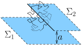
Figure 3: Sketch of the configuration of a semi-infinite plate parallel to an infinite plate at a distance $a$. A worldline can intersect both plates even if its center of mass is located outside the two plates.

In this case, the dominant contribution to the force is given by the universal classic parallel-plate result of Eq. (1) with $A$ being the surface area of the smaller plate.

In the ideal limit of $A$ as well as the edge length $L$ going to infinity, the sub-leading Casimir edge effect is also universal. Dimensional analysis requires the exact force to be of the form

$$F=F_{\|}-\gamma_{\mathrm{1si}}\,\frac{\hbar c}{a^{3}}\,L,$$ (6)

where $F_{\|}$ denotes the parallel-plate force for the Dirichlet scalar, i.e., without the factor 2 in Eq. (1). A priori, the universal coefficient $\gamma_{\mathrm{1si}}$ can be positive or negative. The sign can easily be guessed within the worldline picture: owing to their spatial extent, a sizable fraction of worldlines can intersect both plates even if their center of mass is located outside the plates. This can quantitatively be verified by the energy density, the peak of which indeed extends into the outside region; see Fig. 4.

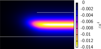
Figure 4: Contour plot of the Casimir interaction energy density $\varepsilon$ for a semi-infinite plate parallel to an infinite plate. The white lines mark the position of the plates to guide the eye. The energy-density peak extends into the outside region, since worldlines can intersect both plates even if their center of mass is in the outside region. Ensemble parameters: 1000 loops, 10 000 ppl.

This peak in the outside region contributes to the total interaction energy, implying an increase of the Casimir force compared to the pure parallel-plate formula. Therefore, the Casimir edge effect leads to further attraction, and the sign of the universal coefficient $\gamma_{\mathrm{1si}}$ must be positive. Quantitatively, we find

$$\gamma_{\mathrm{1si}}=5.23(2)\times 10^{-3},$$ (7)

again with 40 000 loops, 200 000 ppl.

II.3 Parallel semi-infinite plates

Another variant of the parallel-plate configuration is given by two parallel semi-infinite plates with parallel edges; see Fig. 5. This configuration corresponds to an idealized parallel-plate experiment where both plates have the same area size $A$.

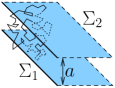
Figure 5: Sketch of the configuration with two parallel semi-infinite plates at a distance $a$.

In the ideal limit of infinite $A$ as well as infinite edge length $L$, the exact form of the force is again given by dimensional analysis,

$$F=F_{\|}-\gamma_{\mathrm{2si}}\,\frac{\hbar c}{a^{3}}\,L,$$ (8)

equivalent to Eq. (6). Qualitatively, the situation is similar to the preceding one with one semi-infinite plate. Quantitatively, fewer worldlines in the outside as well as the inside region near the edge intersect both plates. Both aspects are visible in the plot of the interaction energy density in Fig. 6: the peak height and width is reduced near the edge both inside and outside the plates.

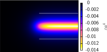
Figure 6: Contour plot of the Casimir interaction energy density $\varepsilon$ for two parallel semi-infinite plates. The energy-density peak extends into the outside region, since worldlines can intersect both plates even if their center of mass is in the outside region. Ensemble parameters: 2000 loops, 10 000 ppl.

We still observe a positive universal coefficient,

$$\gamma_{\mathrm{2si}}=2.30(1)\times 10^{-3}$$ (9)

(93 000 loops, 500 000 ppl), which is a bit less than half as big as the preceding case with one semi-infinite plate. Again, the Casimir edge effect increases the force in comparison with the pure parallel-plate estimate $F_{\|}$.

III Edge-configuration estimates

The universal results for the idealized configurations presented above can immediately be used to derive estimated predictions for further Casimir configurations.

III.1 Casimir comb

Replicating the perpendicular-plate configuration in the horizontal direction of Figs. 1 and 2, we obtain a stack of semi-infinite plates (a “Casimir comb”) perpendicularly above an infinite plate. Let $d$ be the distance between two neighboring semi-infinite plates, i.e., the distance between two teeth of the comb. In the limit $d\gg a$, we obtain the Casimir force between the Casimir comb and the infinite plate by simply adding the forces for the individual perpendicular plates. The reliability of this approximation is obvious from Fig. 2, which shows that the dominant contribution to the energy is peaked inside a region with length scale $\sim a$. The resulting force is

$$F_{\text{comb}}=-\gamma_{\bot}\,\frac{\hbar c}{a^{3}d}\,A,$$ (10)

with $A=Lnd$ being the total area of a comb with $n$ teeth. For a fixed comb, i.e., fixed $d$, the short-distance Casimir force thus has a weaker dependence on $a$ than for the parallel-plate case. In the opposite limit $d\ll a$, we expect the force between the comb and the plate to rapidly approach that of the parallel-plate case (1). This is because a generic worldline contributing to the force will have a spatial extent of order $a$, such that the finer comb scale $d\ll a$ will not be resolved by the worldline ensemble to first approximation. A similar observation has been made in studies of periodic corrugations Emig:2001dx .

III.2 Finite parallel-plate configurations

In a real parallel-plate experiment, the finite extent of the plates induces edge effects. If the typical length scale $L$ of a plate (such as the edge length of a square plate or the radius of a circular disc) is much larger than the plate distance $a$, our results for the idealized limits studied above can be used within a good approximation. The force law can then be summarized as

$$F=-\gamma_{\|}\,\frac{\hbar c}{a^{4}}\,A_{\text{eff}},$$ (11)

where the effective area $A_{\text{eff}}$ also carries the information about the edge effects. For the case of a smaller plate with area $A$ and circumference $C$ above a much larger substrate, the effective area is given by

$$A_{\text{eff}}=A+\frac{\gamma_{\mathrm{1si}}}{\gamma_{\|}}\,aC,$$ (12)

e.g., $C=4L$ for a square plate with edge length $L$. For the case of two parallel plates of equal size and shape with area $A$ and circumference $C$, Eq. (12) holds with $\gamma_{\mathrm{1si}}$ replaced by $\gamma_{\mathrm{2si}}$. Obviously, the effective area $A_{\text{eff}}$ is larger than the physical area in either case.

Consider, for instance, a square plate of edge length $L$ above a larger substrate: the Casimir edge effects induce a correction on the 1% level if $a\gtrsim 1$% of $L$. In the experiment of reference Bressi:2002fr , the edge length is $L=1.2\mathrm{mm}$ and the distance goes up to $a=3\mu\mathrm{m}$. One of the edges faces an edge of the substrate, similar to Fig. 5, whereas the other three correspond to Fig. 3. For the Dirichlet scalar this results in a correction of 0.2%, which is much smaller than the 15% precision level of the experiment.

IV Conclusions

We have performed a detailed quantitative study of Casimir edge effects induced by a fluctuating scalar field obeying Dirichlet boundary conditions. All of our results exhibit a uniquely fixed dependence on dimensionful scales, as for Casimir’s classic result. The effect of quantum fluctuations is quantitatively encoded in a universal dimensionless coefficient, which only depends on the geometry, the nature of the fluctuating field and the boundary conditions. From the perspective of a scattering-theory approach, Casimir edge effects are dominated by diffractive contributions to the correlation functions which are difficult to handle for direct approximation techniques semicl ; Scardicchio:2004fy ; hence, our results give an important first insight into the properties of diffractive contributions to Casimir forces. For Casimir measurements involving electromagnetic fluctuations, our results serve as a first order-of-magnitude estimate of the error induced by edges of finite configurations – an error that any parallel-plate experiment has to deal with.

The authors acknowledge support by the DFG Gi 328/1-3 (Emmy-Noether program) and Gi 328/3-2.

References

- (1) H.B.G. Casimir, Kon. Ned. Akad. Wetensch. Proc. 51, 793 (1948).
- (2) G.L. Klimchitskaya, A. Roy, U. Mohideen, and V.M. Mostepanenko, Phys. Rev. A 60, 3487 (1999).
- (3) A. Lambrecht and S. Reynaud, Eur. Phys. J. D 8, 309 (2000).
- (4) M. Boström and Bo E. Sernelius, Phys. Rev. Lett. 84, 4757 (2000); for a controversial discussion of thermal corrections, see I. Brevik, S. A. Ellingsen and K. A. Milton, arXiv:quant-ph/0605005; V. M. Mostepanenko et al., arXiv:quant-ph/0512134. .
- (5) V.B. Bezerra, G.L. Klimchitskaya, and V.M. Mostepanenko, Phys. Rev. A 62, 014102 (2000).
- (6) M. Bordag, U. Mohideen and V. M. Mostepanenko, Phys. Rept. 353, 1 (2001).
- (7) K. A. Milton, “The Casimir effect: Physical manifestations of zero-point energy”, World Scientific (2001).
- (8) P.A. Maia Neto, A. Lambrecht, and S. Reynaud, Europhys. Lett. 69, 924 (2005); Phys. Rev. A 72, 012115 (2005).
- (9) S. K. Lamoreaux, Phys. Rev. Lett. 78, 5 (1997).
- (10) U. Mohideen and A. Roy, Phys. Rev. Lett. 81, 4549 (1998);
- (11) A. Roy, C. Y. Lin and U. Mohideen, Phys. Rev. D 60, 111101 (1999).
- (12) T. Ederth, Phys. Rev. A 62, 062104 (2000)
- (13) H.B. Chan, V.A. Aksyuk, R.N. Kleiman, D.J. Bishop and F. Capasso, Science 291, 1941 (2001).
- (14) F. Chen, U. Mohideen, G.L. Klimchitskaya and V.M. Mostepanenko, Phys. Rev. Lett. 88, 101801 (2002).
- (15) R.S. Decca, E. Fischbach, G.L. Klimchitskaya, D.E. Krause, D.L. Lopez and V.M. Mostepanenko, Phys. Rev. D 68, 116003 (2003),
- (16) H. Gies and K. Langfeld, Nucl. Phys. B 613, 353 (2001); Int. J. Mod. Phys. A 17, 966 (2002).
- (17) see, e.g., C. Schubert, Phys. Rept. 355, 73 (2001).
- (18) H. Gies, K. Langfeld and L. Moyaerts, JHEP 0306, 018 (2003); arXiv:hep-th/0311168.
- (19) H. Gies and K. Klingmuller, J. Phys. A 39, 6415 (2006).
- (20) H. Gies and K. Klingmuller, Phys. Rev. Lett. 96, 220401 (2006).
- (21) A. Bulgac, P. Magierski and A. Wirzba, Phys. Rev. D 73, 025007 (2006); A. Wirzba, A. Bulgac and P. Magierski, J. Phys. A 39, 6815 (2006).
- (22) T. Emig, R. L. Jaffe, M. Kardar and A. Scardicchio, Phys. Rev. Lett. 96, 080403 (2006).
- (23) M. Bordag, arXiv:hep-th/0602295.
- (24) D.C. Roberts and Y. Pomeau, Phys. Rev. Lett. 95, 145303 (2005); cond-mat/0503757.
- (25) N. Graham, R. L. Jaffe, V. Khemani, M. Quandt, M. Scandurra and H. Weigel, Nucl. Phys. B 645, 49 (2002).
- (26) H. Gies and K. Klingmuller, arXiv:quant-ph/0605141.
- (27) G. Bressi, G. Carugno, R. Onofrio and G. Ruoso, Phys. Rev. Lett. 88, 041804 (2002).
- (28) T. Emig, A. Hanke, R. Golestanian and M. Kardar, Phys. Rev. Lett. 87, 260402 (2001); Phys. Rev. A 67, 022114 (2003); T. Emig, Europhys. Lett. 62, 466 (2003).
- (29) M. Schaden and L. Spruch, Phys. Rev. A 58, 935 (1998); Phys. Rev. Lett. 84 459 (2000) .
- (30) A. Scardicchio and R. L. Jaffe, Nucl. Phys. B 704, 552 (2005); Phys. Rev. Lett. 92, 070402 (2004).
- (31) M. Brown-Hayes, D.A.R. Dalvit, F.D. Mazzitelli, W.J. Kim and R. Onofrio, Phys. Rev. A 72, 052102 (2005).