Two-atom van der Waals interaction between polarizable/magnetizable atoms near magneto-electric bodies

Abstract

The van der Waals potential of two atoms in the presence of an arbitrary arrangement of dispersing and absorbing magneto-electric bodies is studied. Starting from a polarizable atom placed within a given geometry, its interaction with a second polarizable/magnetizable atom is deduced from its Casimir-Polder interaction with a weakly polarizable/magnetizable test body. The general expressions for the van der Waals potential hence obtained are illustrated by considering first the case of two atoms in free space, with special emphasis on the interaction between (i) two polarizable atoms and (ii) a polarizable and a magnetizable atom. Furthermore, the influence of magneto-electric bodies on the van der Waals interaction is studied in detail for the example of two atoms placed near a perfectly reflecting plate or a magneto-electric half space, respectively.

I Introduction

The van der Waals (vdW) interaction of two neutral, unpolarized, but polarizable atoms is a well-known consequence of quantum ground-state fluctuations. For sufficiently small separations, its physical origin may be seen in the electrostatic Coulomb interaction of the atoms’ fluctuating dipole moments. The vdW interaction was first calculated in this nonretarded limit by London on the basis of perturbation theory, who found an attractive potential proportional to $r^{-6}$, where $r$ denotes the interatomic separation lon . For larger separations, the vacuum fluctuations of the (transverse) electromagnetic field also contribute to the interaction. This was first taken into account by Casimir and Polder by means of a normal-mode expansion of the electromagnetic field, generalizing the London potential to arbitrary distances and showing that in particular in the retarded limit the potential varies as $r^{-7}$ c-p .

The theory has since been extended with many respects, and various factors affecting the vdW interaction have been studied. It has been shown that in the case of one pass1 or both atoms p-t3 ; shr being excited, the vdW potential varies as $r^{-6}$ and $r^{-2}$ in the nonretarded and retarded limits, respectively. Thermal photons present for finite temperature have been found to lead to a change of the retarded vdW potential of two ground-state atoms from a $r^{-7}$- to a $r^{-6}$-dependence as soon as the interatomic separation exceeds the wavelength of the dominant photons nin ; wen ; gdk ; bar . The influence of external electric fields on the vdW interaction was addressed, where it has been found that the resulting potential varies as $r^{-3}$ in the nonretarded limit when the applied field is unidirectional mil . Generalizations of the vdW interaction to the three- Axilrod43 ; Aub60 ; Cirone96 ; pass2 and $N$-atom case p-t1 ; p-t2 were studied first in the nonretarded limit and later for arbitrary interatomic separations, where the potentials were seen to depend on the relative positions of the atoms in a rather complicated way.

The two-atom vdW interaction may be strongly affected by the presence of magneto-electric bodies. This was first demonstrated by Mahanty and Ninham, who employed a semiclassical approach to obtain a general expression for the vdW potential of two ground-state atoms in the presence of electric bodies Mahanty72 ; mah ; mah1976 , and applied it to the case of two atoms placed between two perfectly conducting plates mah . The situation of two atoms between two perfectly conducting plates was later reconsidered taking into account finite temperature effects bos . Other scenarios such as two atoms placed within a planar electric three-layer geometry mar or two anisotropic molecules in front of an electric half space or within a planar electric cavity have also been studied Cho .

Bearing in mind that the vdW potential of two polarizable atoms may be modified due to finite temperature, external fields, or the presence of electric bodies, but remains attractive in all of these cases, it is rather surprising that the interaction of a polarizable atom with a magnetizable one is repulsive. This was first realized by Feinberg and Sucher who restricted their attention to the retarded case and found a repulsive potential proportional to $r^{-7}$ feinberg . Their result was later extended to all distances Boyer69 ; Feinberg70 , and in particular it was shown that the nonretarded potential is proportional to $r^{-4}$ Farina02 .

Van der Waals interactions of two atoms exhibiting electric as well as magnetic properties have so far only been studied in the free-space case. A much richer range of phenomena is to be expected when allowing for the presence of magneto-electric bodies, where a complex interplay of the electric and magnetic properties of the atoms and the bodies influences both sign and functional dependence of the two-atom vdW potential. This problem is addressed in the current work, where we derive the vdW potential of a polarizable atom with another polarizable or magnetizable one by starting from its Casimir-Polder (CP) interaction with a weakly polarizable or magnetizable body, respectively. This approach, which has the advantage of being much simpler than perturbative methods and easily applicable to magnetizable atoms, renders general expressions for the two-atom vdW potentials of polarizable and/or magnetizable atoms in the presence of an arbitrary arrangement of magneto-electric bodies, as is shown in Sec. II. In Sec. III, the general results are applied to the vdW interaction between polarizable/magnetizable atoms in free space and in front of a magneto-electric plate. A summary is given in Sec. IV.

II General theory

Consider first a neutral, nonpolar, ground-state atom or molecule $A$ (briefly referred to as atom in the following) in the presence of an arbitrary arrangement of dispersing and absorbing magneto-electric bodies. The atom is characterized by its center-of-mass position $\mathbf{r}_{A}$ and its frequency-dependent electric polarizability $\alpha_{A}(\omega)$, while the bodies are given by their macroscopic (relative) permittivity $\varepsilon(\mathbf{r},\omega)$ and permeability $\mu(\mathbf{r},\omega)$, which are spatially varying, complex-valued functions of frequency, with the corresponding Kramers-Kronig relations being satisfied.

Due to the presence of the bodies, the atom will be subject to a CP force $\mathbf{F}_{A}$. Within the framework of macroscopic QED in linear, causal media and by using leading-order perturbation theory, it can be shown that this force follows from the associated potential Buhmann04 ; Buhmann05

$$U_{A}(\mathbf{r}_{\mathrm{A}})=\frac{\hbar\mu_{0}}{2\pi}\int_{0}^{\infty}\mathrm{d}u\,u^{2}\alpha_{A}(iu)\,\mathrm{Tr}\,\bm{G}^{(1)}(\mathbf{r}_{A},\mathbf{r}_{A},iu)$$ (1)

according to

$$\mathbf{F}_{A}=-\bm{\nabla}_{\!A}U_{A}(\mathbf{r}_{A})$$ (2)

($\bm{\nabla}_{\!A}$ $\!\equiv$ $\!\bm{\nabla}_{\!\mathbf{r}_{A}}$). In Eq. (1), $\bm{G}^{(1)}(\mathbf{r},\mathbf{r}^{\prime},\omega)$ is the scattering part of the classical Green tensor of the electromagnetic field,

$$\bm{G}(\mathbf{r},\mathbf{r}^{\prime},\omega)=\bm{G}^{(0)}(\mathbf{r},\mathbf{r}^{\prime},\omega)+\bm{G}^{(1)}(\mathbf{r},\mathbf{r}^{\prime},\omega)$$ (3)

[$\bm{G}^{(0)}(\mathbf{r},\mathbf{r}^{\prime},\omega)$, bulk part], which is the solution to the equation

$$\biggl{[}\bm{\nabla}\times\kappa(\mathbf{r},\omega)\bm{\nabla}\times\,-\frac{\omega^{2}}{c^{2}}\,\varepsilon(\mathbf{r},\omega)\biggr{]}\bm{G}(\mathbf{r},\mathbf{r}^{\prime},\omega)=\bm{\delta}(\mathbf{r}-\mathbf{r}^{\prime})$$ (4)

[$\kappa(\mathbf{r},\omega)$ $\!=$ $\!\mu^{-1}(\mathbf{r},\omega)$] together with the boundary condition

$$\bm{G}(\mathbf{r},\mathbf{r}^{\prime},\omega)\to 0\quad\mbox{for}\quad|\mathbf{r}-\mathbf{r}^{\prime}|\to\infty.$$ (5)

In order to derive the vdW interaction of atom $A$ with a second polarizable atom $B$, we now introduce an additional, weakly polarizable body of (small) volume $V_{\mathrm{b}}$, consisting of a collection of atoms of type $B$. Provided that the atomic number density $\eta_{B}(\mathbf{r})$ is sufficiently small, the electric susceptibility of the additional body can be approximated by

$$\chi_{\mathrm{e}}(\mathbf{r},\omega)=\begin{cases}\varepsilon_{0}^{-1}\eta_{B}(\mathbf{r})\alpha_{B}(\omega)&\mbox{if }\mathbf{r}\in V_{\mathrm{b}},\\ 0&\mbox{if }\mathbf{r}\not\in V_{\mathrm{b}},\end{cases}$$ (6)

so that the permittivity of the total arrangement of bodies reads $\varepsilon(\mathbf{r},\omega)$ $\!+$ $\!\chi_{\mathrm{e}}(\mathbf{r},\omega)$, and the corresponding Green tensor is given by Eq. (4) with $\varepsilon(\mathbf{r},\omega)$ $\!+$ $\!\chi_{\mathrm{e}}(\mathbf{r},\omega)$ instead of $\varepsilon(\mathbf{r},\omega)$. A linear expansion of this differential equation in terms of $\chi_{\mathrm{e}}$ reveals that the presence of the additional body leads to a change of the Green tensor, whose leading term is

$$\Delta\bm{G}(\mathbf{r},\mathbf{r}^{\prime},\omega)$$

$$\quad=\Bigl{(}\frac{\omega}{c}\Bigr{)}^{2}\int\mathrm{d}^{3}s\,\chi_{\mathrm{e}}(\mathbf{s},\omega)\bm{G}(\mathbf{r},\mathbf{s},\omega)\!\cdot\!\bm{G}(\mathbf{s},\mathbf{r}^{\prime},\omega).$$ (7)

According to Eq. (1), the resulting change of the CP potential is

$$\Delta U_{A}(\mathbf{r}_{A})= -\frac{\hbar}{2\pi\varepsilon_{0}}\int_{0}^{\infty}\mathrm{d}u\,\Bigl{(}\frac{u}{c}\Bigr{)}^{4}\alpha_{A}(iu)\int\mathrm{d}^{3}s\,\chi_{\mathrm{e}}(\mathbf{s},iu)$$

$$\times\mathrm{Tr}\bigl{[}\bm{G}(\mathbf{r}_{A},\mathbf{s},iu)\!\cdot\!\bm{G}(\mathbf{s},\mathbf{r}_{A},iu)\bigr{]}.$$ (8)

Recalling Eq. (6), on can easily see that $\Delta U_{A}$ is just an integral over two-atom potentials $U_{AB}(\mathbf{r}_{A},\mathbf{r}_{B})$,

$$\Delta U_{A}(\mathbf{r}_{A})=\int_{V_{\mathrm{b}}}\mathrm{d}^{3}r_{B}\,\eta_{B}(\mathbf{r}_{B})U_{AB}(\mathbf{r}_{A},\mathbf{r}_{B}),$$ (9)

where

$$U_{AB}(\mathbf{r}_{A},\mathbf{r}_{B})=-\frac{\hbar}{2\pi\varepsilon_{0}^{2}}\int_{0}^{\infty}\mathrm{d}u\,\Bigl{(}\frac{u}{c}\Bigr{)}^{4}\alpha_{A}(iu)\alpha_{B}(iu)\\ \times\mathrm{Tr}\bigl{[}\bm{G}(\mathbf{r}_{A},\mathbf{r}_{B},iu)\!\cdot\!\bm{G}(\mathbf{r}_{B},\mathbf{r}_{A},iu)\bigr{]}.$$ (10)

is the vdW potential between two polarizable atoms in the presence of an arbitrary arrangement of dispersing and absorbing magneto-electric bodies. The total force acting on atom $A$($B$) due to atom $B$($A$) and the bodies is just the sum of the single-atom CP force (2) and the two-atom vdW force

$$\mathbf{F}_{AB(BA)}=-\bm{\nabla}_{\!A(B)}U_{AB}(\mathbf{r}_{A},\mathbf{r}_{B}),$$ (11)

where in general $\mathbf{F}_{AB}$ $\!\neq$ $-\mathbf{F}_{BA}$, due to the presence of the bodies. Equation (10) agrees with the result obtained on the basis of fourth-order perturbation theory, with the perturbative calculation being much more lengthy Buhmann06 ; Safari06 . Needless to say that the method presented here can be easily extended to derive $N$-atom potentials Buhmann06 ; Buhmann06b , whereas the perturbative method becomes increasingly cumbersome for large $N$.

The vdW potential between a polarizable atom $A$ and a magnetizable atom $B$ can be derived in a very analogous way. Again we start from atom $A$ placed within an arbitrary arrangement of magneto-electric bodies, Eqs. (1) and (4), but this time we add a weakly magnetizable body, consisting of a collection of magnetizable atoms of type $B$. For sufficiently small atomic number density the magnetic susceptibility of this body approximately reads

$$\chi_{\mathrm{m}}(\mathbf{r},\omega)=\begin{cases}\mu_{0}\eta_{B}(\mathbf{r})\beta_{B}(\omega)&\mbox{if }\mathbf{r}\in V_{\mathrm{b}},\\ 0&\mbox{if }\mathbf{r}\not\in V_{\mathrm{b}},\end{cases}$$ (12)

with $\beta_{B}(\omega)$ denoting the magnetizability. The inverse permeability of the total arrangment of bodies reads $\kappa(\mathbf{r},\omega)$ $\!-$ $\!\chi_{\mathrm{m}}(\mathbf{r},\omega)$, so that the Green tensor corresponding to this arrangement is given by Eq. (4) with $\kappa(\mathbf{r},\omega)$ $\!-$ $\!\chi_{\mathrm{m}}(\mathbf{r},\omega)$ instead of $\kappa(\mathbf{r},\omega)$. A linear expansion in terms of $\chi_{\mathrm{m}}(\mathbf{r},\omega)$ leads to

$$\Delta\bm{G}(\mathbf{r},\mathbf{r}^{\prime},\omega)=\\ -\int\mathrm{d}^{3}s\,\chi_{\mathrm{m}}(\mathbf{s},\omega)\bigl{[}\bm{G}(\mathbf{r},\mathbf{s},\omega)\!\times\!\overleftarrow{\bm{\nabla}}_{\!\mathbf{s}}\bigr{]}\cdot\!\bm{\nabla}_{\!\mathbf{s}}\!\times\!\bm{G}(\mathbf{s},\mathbf{r}^{\prime},\omega).$$ (13)

Combining this with Eq. (1), we find that the change in the CP potential due to the presence of the additional magnetizable body is

$$\Delta U_{A}(\mathbf{r}_{A})=-\frac{\hbar}{2\pi\varepsilon_{0}}\int_{0}^{\infty}\!\!\mathrm{d}u\,\Bigl{(}\frac{u}{c}\Bigr{)}^{2}\alpha_{A}(iu)\int\!\mathrm{d}^{3}s\,\chi_{\mathrm{m}}(\mathbf{s},iu)$$

$$\quad\times\mathrm{Tr}\Bigl{\{}\bigl{[}\bm{G}(\mathbf{r}_{A},\mathbf{s},iu)\!\times\!\overleftarrow{\bm{\nabla}}_{\!\mathbf{s}}\bigr{]}\!\cdot\!\bm{\nabla}_{\!\mathbf{s}}\!\times\!\bm{G}(\mathbf{s},\mathbf{r}_{A},iu)\Bigr{\}}.$$ (14)

Finally, upon using Eq. (12), Eq. (II) can be rewritten in the form of Eq. (9), where now

$$U_{AB}(\mathbf{r}_{A},\mathbf{r}_{B})=-\frac{\hbar\mu_{0}}{2\pi\varepsilon_{0}}\int_{0}^{\infty}\mathrm{d}u\,\Bigl{(}\frac{u}{c}\Bigr{)}^{2}\alpha_{A}(iu)\beta_{B}(iu)$$

$$\quad\times\mathrm{Tr}\bigl{[}\bm{G}(\mathbf{r}_{A},\mathbf{r},iu)\!\times\!\overleftarrow{\bm{\nabla}}_{\!\mathbf{r}}\!\cdot\!\bm{\nabla}_{\!\mathbf{r}}\!\times\!\bm{G}(\mathbf{r},\mathbf{r}_{A},iu)\bigr{]}_{\mathbf{r}=\mathbf{r}_{B}}$$ (15)

is the vdW potential between a polarizable atom $A$ and a magnetizable atom $B$ in the presence of an arbitrary arrangement of magneto-electric bodies. To our knowledge, Eq. (II) has never been derived so far.

III Examples

III.1 Free space

In order to illustrate the two-atom vdW potentials (10) and (II), let us first consider two atoms in free space, with the Green tensor being given by Knoll01

$$\bm{G}^{(0)}(\mathbf{r},\mathbf{r}^{\prime},iu)=\frac{e^{-u\rho/c}}{4\pi\rho}\bigl{\{}a[c/(u\rho)]\bm{I}-b[c/(u\rho)]\mathbf{e}_{\rho}\mathbf{e}_{\rho}\bigr{\}},$$ (16)

$$a(x)=1+x+x^{2},\qquad b(x)=1+3x+3x^{2}$$ (17)

($\bm{\rho}$ $\!\equiv$ $\!\mathbf{r}-\mathbf{r}^{\prime}$; $\rho$ $\!\equiv$ $\!|\bm{\rho}|$; $\mathbf{e}_{\rho}$ $\!\equiv$ $\!\bm{\rho}/\rho$; $\bm{I}$, unit tensor). In this case, the vdW potential between two polarizable atoms, Eq. (10), reads

$$U^{(0)}_{AB}(\mathbf{r}_{A},\mathbf{r}_{B})=-\frac{\hbar}{32\pi^{3}\varepsilon_{0}^{2}l^{6}}\int_{0}^{\infty}\!\mathrm{d}u\,\alpha_{A}(iu)\alpha_{B}(iu)g(ul/c),$$ (18)

$$g(x)=2e^{-2x}(3+6x+5x^{2}+2x^{3}+x^{4})$$ (19)

($l$ $\!\equiv$ $|\mathbf{r}_{A}-\mathbf{r}_{B}|$), in agreement with the well-known result of Casimir and Polder c-p . From

$$\bm{\nabla}\biggl{[}\frac{g(ur/c)}{r^{6}}\biggr{]}= -\frac{4\hat{\mathbf{r}}}{r^{7}}\bigl{[}e^{-2x}(9+18x+16x^{2}$$

$$+8x^{3}+3x^{4}+x^{5})\bigr{]}_{x=ur/c}$$ (20)

it can be seen that the potential (18) is always attractive.

In the retarded limit, where $l$ $\!\gg$ $\!c/\omega_{\mathrm{min}}$ ($\omega_{\mathrm{min}}$ denoting the minimum of all resonance frequencies of atoms $A$ and $B$) the exponential factor effectively limits the $u$-integral in Eq. (18) to a region where

$$\alpha_{A}(iu)\simeq\alpha_{A}(0),\quad\alpha_{B}(iu)\simeq\alpha_{B}(0),$$ (21)

hence the integral can be performed in closed form to yield

$$U^{(0)}_{AB}(\mathbf{r}_{A},\mathbf{r}_{B})=-\frac{C_{7}}{l^{7}}\,,$$ (22)

$$C_{7}=\frac{23\hbar c\alpha_{A}(0)\alpha_{B}(0)}{64\pi^{3}\varepsilon_{0}^{2}}\,.$$ (23)

In the opposite, nonretarded limit, where $l$ $\!\ll$ $\!c/\omega_{\mathrm{max}}$ ($\omega_{\mathrm{max}}$ denoting the maximum of all resonance frequencies of atoms $A$ and $B$), the factors $\alpha_{A}(iu)$ and $\alpha_{B}(iu)$ effectively limit the $u$-integral in Eq. (18) to a region where

$$g(ul/c)\simeq g(0)=6,$$ (24)

so that the London potential lon is recovered,

$$U^{(0)}_{AB}(\mathbf{r}_{A},\mathbf{r}_{B})=-\frac{C_{6}}{l^{6}}\,,$$ (25)

$$C_{6}=\frac{3\hbar}{16\pi^{3}\varepsilon_{0}^{2}}\int_{0}^{\infty}{\rm d}u\,\alpha_{A}(iu)\alpha_{B}(iu).$$ (26)

To calculate the potential between a polarizable atom and a magnetizable one, we first use Eq. (16) to derive

$$\bm{\nabla}\!\times\!\bm{G}^{(0)}(\mathbf{r},\mathbf{r}^{\prime},iu)=-\frac{e^{-\frac{u\rho}{c}}}{4\pi\rho^{2}}\Bigl{(}1+\frac{u\rho}{c}\Bigr{)}\mathbf{e}_{\rho}\!\times\!\bm{I},$$ (27)

$$\bm{G}^{(0)}(\mathbf{r},\mathbf{r}^{\prime},iu)\!\times\!\overleftarrow{\bm{\nabla}}{}^{\prime}=\frac{e^{-\frac{u\rho}{c}}}{4\pi\rho^{2}}\Bigl{(}1+\frac{u\rho}{c}\Bigr{)}\bm{I}\!\times\!\mathbf{e}_{\rho}.$$ (28)

Substituting Eqs. (27) and (28) into Eq. (II) and using the identity

$$\mathrm{Tr}\bigl{[}\mathbf{e}_{\rho}\!\times\!\bm{I}\!\times\!\mathbf{e}_{\rho}\bigr{]}=-2,$$ (29)

we find that

$$U_{AB}^{(0)}(\mathbf{r}_{A},\mathbf{r}_{B})=\\ \frac{\hbar\mu_{0}}{32\pi^{3}\varepsilon_{0}l^{4}}\int_{0}^{\infty}\mathrm{d}u\,\Bigl{(}\frac{u}{c}\Bigr{)}^{2}\alpha_{A}(iu)\beta_{B}(iu)h(ul/c),$$ (30)

$$h(x)=2e^{-2x}(1+2x+x^{2}),$$ (31)

in agreement with results found earlier Boyer69 ; Feinberg70 .

In contrast to the attractive vdW potential between two polarizable atoms, Eq. (18), the vdW potential between a polarizable and a magnetizable atom, Eq. (30), is always repulsive, as can be seen from

$$\bm{\nabla}\biggl{[}\frac{h(ur/c)}{r^{4}}\biggr{]}=-\frac{4\hat{\mathbf{r}}}{r^{5}}\bigl{[}e^{-2x}(2+4x+3x^{2}+x^{3})\bigr{]}_{x=ur/c}.$$ (32)

In particular, one finds, on using Eqs. (21) and

$$h(ul/c)\simeq h(0)=2,$$ (33)

that Eq. (30) reduces to

$$U_{AB}^{(0)}(\mathbf{r}_{A},\mathbf{r}_{B})=\frac{C_{7}}{l^{7}}\,,$$ (34)

$$C_{7}=\frac{7\hbar c\mu_{0}\alpha_{A}(0)\beta_{B}(0)}{64\pi^{3}\varepsilon_{0}}$$ (35)

and

$$U_{AB}^{(0)}(\mathbf{r}_{A},\mathbf{r}_{B})=\frac{C_{4}}{l^{4}}\,,$$ (36)

$$C_{4}=\frac{\hbar\mu_{0}}{16\pi^{3}\varepsilon_{0}}\int_{0}^{\infty}\mathrm{d}u\,\Bigl{(}\frac{u}{c}\Bigr{)}^{2}\alpha_{A}(iu)\beta_{B}(iu)$$ (37)

in the retarded and nonretarded limits, respectively. The vdW potential between a polarizable atom and a magnetizable one hence shows a $l^{-7}$ power law in the nonretarded limit which is weaker than the corresponding $l^{-7}$ vdW potential of two polarizable atoms by a factor of $7/23$; while in the nonretarded limit, the potential between a polarizable and a magnetizable atom follows a $l^{-4}$ power law which is more weakly diverging than the corresponding $l^{-6}$ potential between two polarizable atoms.

III.2 Semi-infinite half space

Let us now study the influence of the presence of magneto-electric bodies on the two-atom vdW potential. To that end, we consider two polarizable atoms placed near a homogeneous semi-infinite half space. We choose the coordinate system such that the $z$ axis is perpendicular to the plate with the origin being on its surface, and the two atoms lie in the $xz$ plane (Fig. 1). In this case, the nonzero elements of the scattering Green tensor are given by (App. A)

$${G}^{(1)}_{xx(yy)}({\mathbf{r}}_{A},{\mathbf{r}}_{B},iu)=\frac{1}{8\pi}\int_{0}^{\infty}{\rm d}q\,qe^{-bZ_{+}}$$

$$\quad\times\biggl{[}\frac{J_{0}(qX)\;\raisebox{2.5pt}{$+$}\raisebox{-2.5pt}{{\scriptsize(}$\!-\!$\scriptsize{)}}\,J_{2}(qX)}{b}\,r_{s}-\frac{b[J_{0}(qX)\;\raisebox{2.5pt}{$-$}\raisebox{-2.5pt}{{\scriptsize(}$\!+\!$\scriptsize{)}}\,J_{2}(qX)]}{k^{2}}\,r_{p}\biggr{]},$$ (38)

$${G}^{(1)}_{xz(zx)}({\mathbf{r}}_{A},{\mathbf{r}}_{B},iu)=\raisebox{2.5pt}{$-$}\raisebox{-2.5pt}{{\scriptsize(}$\!+\!$\scriptsize{)}}\frac{1}{4\pi}\!\int_{0}^{\infty}\!\!{\rm d}q\,q^{2}e^{-bZ_{+}}\frac{J_{1}(qX)}{k^{2}}\,r_{p},$$ (39)

$${G}^{(1)}_{zz}({\mathbf{r}}_{A},{\mathbf{r}}_{B},iu)=-\frac{1}{4\pi}\int_{0}^{\infty}{\rm d}q\,q^{3}e^{-bZ_{+}}\frac{J_{0}(qX)}{bk^{2}}\,r_{p}$$ (40)

[$J_{\nu}(x)$, Bessel function; $Z_{+}$ $\!=$ $\!z_{A}$ $\!+$ $\!z_{B}$; $X$ $\!=$ $\!x_{B}$ $\!-$ $\!x_{A}$], where $r_{\sigma}$ $\!=$ $r_{\sigma}(q,u)$ ($\sigma$ $\!=$ $\!s,p$) are the reflection coefficients of the half space [cf. Eqs. (46), (63) and (64) below], and

$$b=b(q,u)=\sqrt{\frac{u^{2}}{c^{2}}+q^{2}}\,,$$ (41)

$$k=k(q,u)=\frac{u}{c}\,.$$ (42)

According to the decomposition (3) of the Green tensor, the two-atom potential (10) can be split into three parts,

$$U_{AB}(\mathbf{r}_{A},\mathbf{r}_{B})= \,U_{AB}^{(0)}(\mathbf{r}_{A},\mathbf{r}_{B})+U_{AB}^{(1)}(\mathbf{r}_{A},\mathbf{r}_{B})$$

$$+U_{AB}^{(2)}(\mathbf{r}_{A},\mathbf{r}_{B}),$$ (43)

where the bulk-part contribution $U_{AB}^{(0)}(\mathbf{r}_{A},\mathbf{r}_{B})$ is simply the free-space result (18),

$$U_{AB}^{(1)}(\mathbf{r}_{A},\mathbf{r}_{B})=-\frac{\hbar}{\pi\varepsilon_{0}^{2}}\int_{0}^{\infty}{\mathrm{d}}u\,\Bigl{(}\frac{u}{c}\Bigr{)}^{4}\alpha_{A}(iu)\alpha_{B}(iu)$$

$$\quad\times\mathrm{Tr}\big{[}{\bm{G}}^{(0)}(\mathbf{r}_{A},\mathbf{r}_{B},iu)\!\cdot\!{\bm{G}}^{(1)}(\mathbf{r}_{B},\mathbf{r}_{A},iu)\big{]}$$

$$=-\frac{\hbar}{32\pi^{3}\varepsilon_{0}^{2}l}\int_{0}^{\infty}{\mathrm{d}}u\,\Bigl{(}\frac{u}{c}\Bigr{)}^{4}\alpha_{A}(iu)\alpha_{B}(iu)\,e^{-ul/c}$$

$$\quad\times\int_{0}^{\infty}{\rm d}q\,qe^{-bZ_{+}}\left(\bigg{\{}\bigg{[}2f(\xi)-g(\xi)\frac{X^{2}}{l^{2}}\bigg{]}\bigg{[}\frac{r_{s}}{b}-\frac{br_{p}}{k^{2}}\bigg{]}\right.$$

$$\quad-2\bigg{[}f(\xi)-g(\xi)\frac{Z^{2}}{l^{2}}\bigg{]}\frac{q^{2}r_{p}}{bk^{2}}\bigg{\}}J_{0}(qX)$$

$$\quad\left.-g(\xi)\frac{X^{2}}{l^{2}}\bigg{[}\frac{r_{s}}{b}+\frac{br_{p}}{k^{2}}\bigg{]}J_{2}(qX)\right)$$ (44)

comes from the cross term of bulk and scattering parts [with $Z$ $\!=$ $\!z_{B}$ $\!-$ $\!z_{A}$, $\xi$ $\!=$ $\!c/(lu)$, and $a(x)$ and $b(x)$ as given in Eq. (17)], and

$$U_{AB}^{(2)}(\mathbf{r}_{A},\mathbf{r}_{B})=-\frac{\hbar}{2\pi\varepsilon_{0}^{2}}\int_{0}^{\infty}\!{\mathrm{d}}u\,\Bigl{(}\frac{u}{c}\Bigr{)}^{4}\alpha_{A}(iu)\alpha_{B}(iu)$$

$$\quad\times\mathrm{Tr}\big{[}{\bm{G}}^{(1)}(\mathbf{r}_{A},\mathbf{r}_{B},iu)\!\cdot\!{\bm{G}}^{(1)}(\mathbf{r}_{B},\mathbf{r}_{A},iu)\big{]}$$

$$=-\frac{\hbar}{64\pi^{3}\varepsilon_{0}^{2}}\int_{0}^{\infty}\!\!{\mathrm{d}}u\Bigl{(}\frac{u}{c}\Bigr{)}^{4}\alpha_{A}(iu)\alpha_{\mathrm{B}}(iu)\int_{0}^{\infty}\!\!{\rm d}q\,q\int_{0}^{\infty}\!\!{\rm d}q^{\prime}\,q^{\prime}$$

$$\quad\times e^{-(b+b^{\prime})Z_{+}}\biggl{\{}\bigg{[}\frac{r_{s}r^{\prime}_{s}}{bb^{\prime}}+\frac{r_{p}r^{\prime}_{p}}{k^{4}}\bigg{(}bb^{\prime}+\frac{2q^{2}q^{\prime 2}}{bb^{\prime}}\bigg{)}-\frac{b^{\prime}r_{s}r^{\prime}_{p}}{b{k}^{2}}$$

$$\quad-\frac{br_{p}r^{\prime}_{s}}{b^{\prime}{k}^{2}}\bigg{]}J_{0}(qX)J_{0}(q^{\prime}X)+\frac{4qq^{\prime}r_{p}r^{\prime}_{p}}{k^{4}}J_{1}(qX)J_{1}(q^{\prime}X)$$

$$\quad+\bigg{[}\frac{r_{s}r^{\prime}_{s}}{bb^{\prime}}+\frac{bb^{\prime}r_{p}r^{\prime}_{p}}{k^{4}}+\frac{b^{\prime}r_{s}r^{\prime}_{p}}{b{k}^{2}}+\frac{br_{p}r^{\prime}_{s}}{b^{\prime}{k}^{2}}\bigg{]}\!J_{2}(qX)J_{2}(q^{\prime}X)\!\biggr{\}}$$ (45)

is the scattering-part contribution [$b^{\prime}$ $\!=$ $\!b(q^{\prime},u)$, $r^{\prime}_{\sigma}$ $\!=r_{\sigma}(q^{\prime},u)$ for $\sigma$ $\!=$ $\!s,p$].

III.2.1 Perfectly reflecting plate

Figure 1: Two atoms near a perfectly reflecting plate.

For a perfectly reflecting plate, the reflection coefficients are simply given by

$$r_{s}=\mp 1,\qquad r_{p}=\pm 1,$$ (46)

where the upper (lower) sign corresponds to a perfectly conducting (permeable) plate. In the retarded limit, where $l,z_{A},z_{B}$ $\!\gg$ $\!c/\omega_{\mathrm{min}}$, $U_{AB}^{(0)}$ is given by Eq. (22), whereas $U_{AB}^{(1)}$ [Eq. (III.2)] and $U_{AB}^{(2)}$ [Eq. (III.2)] can be given in closed form only in some special cases. If $X$ $\!\ll$ $\!Z_{+}$ (cf. Fig. 1), we derive, on using the relevant elements of the scattering Green tensor as given in App. A [Eqs. (A) and (A)],

$$U_{AB}^{(1)}=\pm\frac{32}{23}\,\frac{(X^{2}+6l^{2})C_{7}}{l^{3}Z_{+}(l+Z_{+})^{5}}\,,$$ (47)

$$U_{AB}^{(2)}=-\frac{C_{7}}{Z_{+}^{7}}\,,$$ (48)

where $C_{7}$ is given by Eq. (23). Thus, recalling Eq. (22), the two-atom vdW potential (III.2) reads

$$U_{AB}=-\frac{C_{7}}{l^{7}}\pm\frac{32}{23}\frac{(X^{2}+6l^{2})C_{7}}{l^{3}Z_{+}(l+Z_{+})^{5}}-\frac{C_{7}}{Z_{+}^{7}}\,.$$ (49)

In particular, if $z_{A}/z_{B}$ $\!\ll$ $\!1$, Eqs. (47) and (48) imply that

$$U_{AB}^{(1)}=\mp\frac{6}{23}\,U_{AB}^{(0)}\,,$$ (50)

$$U_{AB}^{(2)}=U_{AB}^{(0)}\,,$$ (51)

so the presence of the perfectly reflecting plate leads to an enhancement of the interaction potential,

$$U_{AB}=\begin{cases}\displaystyle\frac{40}{23}\,U_{AB}^{(0)},\\[8.61108pt] \displaystyle\frac{52}{23}\,U_{AB}^{(0)}\end{cases}$$ (52)

for a perfectly conducting or permeable plate, respectively.

Quite generally, since the bulk part $U_{AB}^{(0)}$ [first term on the r.h.s. of Eq. (49)] is negative, the interaction potential is enhanced (reduced) by the plate if the scattering part $U_{AB}^{(1)}\!+\!U_{AB}^{(2)}$ [second and third terms on the r.h.s. of Eq. (49)] is negative (positive). In the case of a perfectly conducting plate, it is seen that especially for $Z$ $\!=$ $\!0$, briefly referred to as the parallel case, $U_{AB}^{(1)}\!+\!U_{AB}^{(2)}$ is positive, and hence the interaction potential is reduced by the plate, whereas for $X$ $\!=$ $\!0$, briefly referred to as the vertical case, $U_{AB}^{(1)}\!+\!U_{AB}^{(2)}$ is positive and the interaction potential is reduced iff

$$z_{B}/z_{A}\lesssim 4.90,$$ (53)

where, without loss of generality, atom $A$ is assumed to be closer to the plate than atom $B$. It is apparent from Eq. (49) that for a perfectly permeable plate $U_{AB}^{(1)}\!+\!U_{AB}^{(2)}$ is always negative, and hence the interaction potential is always enhanced by the plate.

In the nonretarded limit, where $l,z_{A},z_{B}$ $\!\ll$ $\!c/\omega_{\mathrm{max}}$, $U_{AB}^{(0)}$ is given by Eq. (25), and from Eqs. (III.2) and (III.2) we derive, on making use of the relevant elements of the scattering Green tensor as given in App. A [Eqs. (102)–(105)],

$$U_{AB}^{(1)}=\pm\frac{\bigl{[}4X^{4}-2Z^{2}Z_{+}^{2}+X^{2}(Z_{+}^{2}+Z^{2})\bigr{]}C_{6}}{3l^{5}l_{+}^{5}}\,,$$ (54)

$$U_{AB}^{(2)}=-\frac{C_{6}}{l_{+}^{6}}$$ (55)

($l_{+}$ $\!=$ $\!\sqrt{X^{2}+Z_{+}^{2}}$), where $C_{6}$ is given by Eq. (26). Hence, the interaction potential (III.2), reads, on recalling Eq. (25),

$$U_{AB}=-\frac{C_{6}}{l^{6}}\pm\frac{\bigl{[}4X^{4}\!-\!2Z^{2}Z_{+}^{2}\!+\!X^{2}(Z_{+}^{2}\!+\!Z^{2})\bigr{]}C_{6}}{3l^{5}l_{+}^{5}}-\frac{C_{6}}{l_{+}^{6}}\,.$$ (56)

Let us again consider the effect of the plate on the interaction potential for the parallel and vertical cases. In the parallel case, Eq. (56) takes the form

$$U_{AB}=-\frac{C_{6}}{l^{6}}\pm\frac{(4l^{2}+Z_{+}^{2})C_{6}}{3l^{3}(l^{2}+Z_{+}^{2})^{\frac{5}{2}}}-\frac{C_{6}}{(l^{2}+Z_{+}^{2})^{3}}\,.$$ (57)

which in the on-surface limit $Z_{+}$ $\!\to$ $\!0$ approaches

$$U_{AB}=\begin{cases}\displaystyle\frac{2}{3}\,U_{AB}^{(0)},\\[8.61108pt] \displaystyle\frac{10}{3}\,U_{AB}^{(0)}\end{cases}$$ (58)

for a perfectly conducting or permeable plate, respectively. It can easily be seen that the term $U_{AB}^{(1)}$ [second term on the r.h.s. of Eq. (57)] dominates the term $U_{AB}^{(2)}$ [third term on the r.h.s. of Eq. (57)], so $U_{AB}^{(1)}\!+\!U_{AB}^{(2)}$ is positive (negative) for a perfectly conducting (permeable) plate, and hence the interaction potential is reduced (enhanced) due to the presence of the plate.

In the vertical case, from Eq. (56) the interaction potential is obtained to be

$$U_{AB}=-\frac{C_{6}}{l^{6}}\mp\frac{2C_{6}}{3Z_{+}^{3}l^{3}}-\frac{C_{6}}{Z_{+}^{6}}\,.$$ (59)

It is obvious that $U_{AB}^{(1)}\!+\!U_{AB}^{(2)}$ [second and third terms on the r.h.s. of Eq. (59)] is negative when the plate is perfectly conducting, thereby enhancing the interaction potential since $U_{AB}^{(0)}$ [first term in Eq. (59)] is negative. In the case of a perfectly permeable plate, $U_{AB}^{(1)}\!+\!U_{AB}^{(2)}$ is positive iff

$$\frac{z_{B}}{z_{A}}<1+\frac{2}{(3/2)^{1/3}-1}\simeq 14.82,$$ (60)

where atom $A$ is again assumed to be closer to the plate than atom $B$.

The enhancing/reducing effect of the perfectly reflecting plate on the two-atom vdW potential in the various cases considered can be systematized in a simple way. Since $U_{AB}^{(0)}$ and $U_{AB}^{(2)}$ are negative in all the cases, the enhancement or reduction of the vdW potential due to the presence of the plate depends only on the sign of $U_{AB}^{(1)}$ and its magnitude compared to that of $U_{AB}^{(2)}$.

	conducting plate	permeable plate
parallel case	$+$	$-$
vertical case	$-$	$+$

Table 1: Sign of $U_{AB}^{(1)}$ for a perfectly reflecting plate.

Moreover, the results for the non-retarded limit (the sign of $U_{AB}^{(1)}$ being summarized in Tab. 1) can be explained by using the method of image charges, where the two-atom vdW interaction is regarded as being due to the interactions between fluctuating dipoles $A$ and $B$ and their images ${A}^{\prime}$ and ${B}^{\prime}$ in the plate, with

$$\hat{H}_{\mathrm{int}}=\hat{V}_{AB}+\hat{V}_{AB^{\prime}}+\hat{V}_{BA^{\prime}}$$ (61)

being the corresponding interaction Hamiltonian. Here, $\hat{V}_{AB}$ denotes the direct interaction between dipole $A$ and dipole $B$, while $\hat{V}_{AB^{\prime}}$ and $\hat{V}_{BA^{\prime}}$ denote the indirect interaction between each dipole and the image induced by the other one in the plate. According to this approach, the vdW potential $U_{AB}$ can be identified with the second-order energy shift

$$\Delta E_{AB}=-\sum_{(n,m)\neq(0,0)}\frac{\langle 0_{A}|\langle 0_{B}|\hat{H}_{\mathrm{int}}|n_{A}\rangle|m_{B}\rangle}{\hbar(E_{A}^{n}+E_{B}^{m}-E_{A}^{0}-E_{B}^{0})}\\ \times\,\langle n_{A}|\langle m_{B}|\hat{H}_{\mathrm{int}}|0_{A}\rangle|0_{B}\rangle.$$ (62)

($E_{A(B)}^{n}$, $|n_{A(B)}\rangle$; atomic eigenenergies and eigenstates, respectively). In this approach, $U_{AB}^{(0)}$ corresponds to the product of two direct interactions, so it is negative in agreement with Eq. (56), because of the minus sign on the r.h.s. of Eq. (62). Accordingly, $U_{AB}^{(2)}$ is due to the product of two indirect interactions and is also negative—in agreement with Eq. (56). The terms containing one direct and one indirect interaction are contained in $U^{(1)}_{AB}$ and determine its sign. We can hence predict the sign of $U^{(1)}_{AB}$ from a graphical construction of the image charges, as sketched in Figs. 2–5.

Figure 2 shows two electric dipoles in front of a perfectly conducting plate in the parallel case. The configuration of dipoles and images indicates repulsion between dipole $A(B)$ and dipole $B^{\prime}(A^{\prime})$, so $U_{AB}^{(1)}$ is positive, in agreement with Tab. 1. On the contrary, in the vertical case from Fig. 3 attraction is indicated, i.e., negative $U_{AB}^{(1)}$, which is also in agreement with Tab. 1.

The case of two electric dipoles in front of a perfectly permeable plate can be treated by considering two magnetic dipoles in front of a perfectly conducting plate, as the two situations are equivalent due to the duality between electric and magnetic fields in the absence of free charges or currents. From Figs. 4 (parallel case) and 5 (vertical case) it is apparent that the interaction between dipole $A(B)$ and dipole $B^{\prime}(A^{\prime})$ is attractive in the parallel case and repulsive in the vertical case, again confirming the sign of $U_{AB}^{(1)}$ as given in Tab. 1.

When the dipole–dipole separation in Fig. 5 is sufficiently small compared with the dipole–surface separations, then the direct interaction between the two dipoles is expected to be stronger than their indirect interaction via the image dipoles. As a result, $U_{AB}^{(1)}$ will be the dominant term in $U_{AB}^{(1)}\!+\!U_{AB}^{(2)}$ and $U_{AB}^{(1)}\!+\!U_{AB}^{(2)}$ becomes positive. However, when the dipole–dipole separation exceeds the dipole–surface separations, then the indirect interaction may become comparable to the direct one, and $U_{AB}^{(2)}$ may be the dominant term, leading to negative $U_{AB}^{(1)}\!+\!U_{AB}^{(2)}$. The image dipole model hence gives also a qualitative explanation of the condition (60).

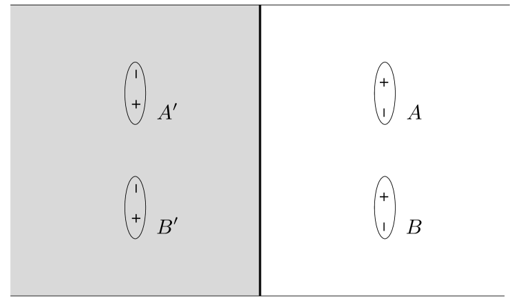
Figure 2: Two electric dipoles near a perfectly conducting plate (parallel case).

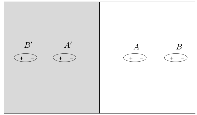
Figure 3: Two electric dipoles near a perfectly conducting plate (vertical case).

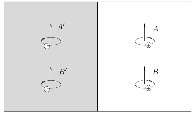
Figure 4: Two magnetic dipoles near a perfectly conducting plate (parallel case).

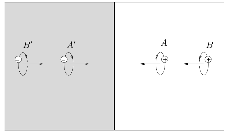
Figure 5: Two magnetic dipoles near a perfectly conducting plate (vertical case).

III.2.2 Magneto-electric half space

Let us now abandon the assumption of perfect reflectivity and consider a magneto-electric half space of permittivity $\varepsilon(\omega)$ and permeability $\mu(\omega)$. In this case, the reflection coefficients in Eqs. (III.2) and (III.2) are given by

$$r_{s}=r_{s}(q,u)=\frac{\mu(iu)b-b_{\mathrm{M}}}{\mu(iu)b+b_{\mathrm{M}}}\,,$$ (63)

$$r_{p}=r_{p}(q,u)=\frac{\varepsilon(iu)b\!-\!b_{\mathrm{M}}}{\varepsilon(iu)b+b_{\mathrm{M}}}\,,$$ (64)

where $b$ is defined by Eq. (41), and

$$b_{\mathrm{M}}=b_{\mathrm{M}}(q,u)=\sqrt{\varepsilon(iu)\mu(iu)\frac{u^{2}}{c^{2}}+q^{2}}\,.$$ (65)

In the retarded limit, $l,z_{A},z_{B}$ $\!\gg$ $\!c/\omega_{\mathrm{min}}$ (where $\omega_{\mathrm{min}}$ now denotes the minimum of all resonance frequencies of atoms $A$ and $B$ and the magneto-electric medium) we may again approximate the atomic polarizabilities by their static values, recall Eq. (21), and similarly we may set

$$\varepsilon(iu)\simeq\varepsilon(0),\qquad\mu(iu)\simeq\mu(0).$$ (66)

Replacing the integration variable $q$ in Eq. (III.2) by $v$ $\!=$ $\!bc/u$ [cf. Eq. (97)], one can show that the contribution $U_{AB}^{(1)}$ to the vdW potential takes the form

$$U_{AB}^{(1)}(\mathbf{r}_{A},\mathbf{r}_{B})=\frac{\hbar c}{32\pi^{3}l^{3}\varepsilon_{0}^{2}}\alpha_{A}(0)\alpha_{B}(0)\int_{1}^{\infty}{\rm d}v\,$$

$$\quad\times\bigg{(}\bigg{\{}v^{2}\bigg{[}Z^{2}A_{5-}+(Z^{2}-2X^{2})\bigg{(}\frac{A_{4-}}{l}+\frac{A_{3-}}{l^{2}}\bigg{)}$$

$$\qquad+l^{2}A_{5+}+lA_{4+}+A_{3+}\bigg{]}+2(v^{2}-1)\bigg{[}X^{2}B_{5}$$

$$\qquad+\big{(}X^{2}-2Z^{2}\big{)}\bigg{(}\frac{B_{4}}{l}+\frac{B_{3}}{l^{2}}\bigg{)}\bigg{]}\bigg{\}}r_{p}$$

$$\qquad+\bigg{[}Z^{2}A_{5+}+\big{(}Z^{2}-2X^{2}\big{)}\bigg{(}\frac{A_{4+}}{l}+\frac{A_{3+}}{l^{2}}\bigg{)}$$

$$\qquad+l^{2}A_{5-}+lA_{4-}+A_{3-}\bigg{]}r_{s}\bigg{)},$$ (67)

where according to Eqs. (63) and (64), the static reflection coefficients are given by

$$r_{s}=r_{s}(v)=\frac{\mu(0)v-\sqrt{\varepsilon(0)\mu(0)-1+v^{2}}}{\mu(0)v+\sqrt{\varepsilon(0)\mu(0)-1+v^{2}}}\,,$$ (68)

$$r_{p}=r_{p}(v)=\frac{\varepsilon(0)v-\sqrt{\varepsilon(0)\mu(0)-1+v^{2}}}{\varepsilon(0)v+\sqrt{\varepsilon(0)\mu(0)-1+v^{2}}}\,,$$ (69)

and

$$A_{k\pm}=\int_{0}^{\infty}\mathrm{d}x\,x^{k}\,e^{-\lambda x}\big{[}J_{0}(\zeta x)\pm J_{2}(\zeta x)\big{]},$$ (70)

$$B_{k}=\int_{0}^{\infty}{\mathrm{d}}x\,x^{k}e^{-\lambda x}J_{0}(\zeta x),$$ (71)

with $\lambda$ $\!=$ $\!l$ $\!+$ $\!vZ_{+}$ and $\zeta$ $\!=$ $\!X\sqrt{v^{2}-1}$ (for explicit expressions of $A_{k\pm}$ and $B_{k}$, see App. B). Similarly, Eq. (III.2) reduces to

$$U_{AB}^{(2)}=-\frac{\hbar c}{64\pi^{3}\varepsilon_{0}^{2}}\,\alpha_{A}(0)\alpha_{B}(0)\int_{1}^{\infty}{\rm d}v\int_{1}^{\infty}{\rm d}v^{\prime}$$

$$\quad\times\biggl{\{}\Big{(}r_{p}r_{p}^{\prime}\big{[}3v^{2}v^{\prime 2}-2(v^{2}+v^{\prime 2})+2\big{]}+r_{s}r_{s}^{\prime}-r_{s}r_{p}^{\prime}v^{\prime 2}$$

$$\quad-r_{p}r_{s}^{\prime}v^{2}\Big{)}M_{0}+4vv^{\prime}\sqrt{v^{2}-1}\sqrt{v^{\prime 2}-1}r_{p}r_{p}^{\prime}M_{1}$$

$$\quad+\big{(}r_{s}r_{s}^{\prime}+r_{p}r_{p}^{\prime}v^{2}v^{\prime 2}+r_{s}r_{p}^{\prime}v^{\prime 2}+r_{p}r_{s}^{\prime}v^{2}\big{)}M_{2}\biggr{\}}$$ (72)

[$r^{\prime}_{\sigma}=r_{\sigma}(v^{\prime})$ for $\sigma$ $\!=$ $\!s,p$], where

$$M_{\nu}=\int_{0}^{\infty}{\mathrm{d}}x\,x^{6}e^{-(v+v^{\prime})Z_{+}x}J_{\nu}(\zeta x)J_{\nu}(\zeta^{\prime}x)$$ (73)

($\zeta^{\prime}$ $\!=$ $\!X\sqrt{v^{\prime 2}-1}$), which can be evaluated analytically only in some special cases. In particular, when $X$ $\!\ll$ $\!Z_{+}$, then approximately

$$M_{\nu}=J_{\nu}^{2}(0)\int_{0}^{\infty}{\mathrm{d}}x\,x^{6}e^{-(v+v^{\prime})Z_{+}x}=\frac{720\delta_{\nu 0}}{(v+v^{\prime})^{7}Z_{+}^{7}}\,.$$ (74)

Analytic expressions for $U_{AB}^{(1)}$ and $U_{AB}^{(2)}$ in the nonretarded limit, $l,z_{A},z_{B}$ $\!\ll$ $\!c/[\sqrt{\varepsilon(0)\mu(0)}\,\omega_{\mathrm{max}}]$ [with $\omega_{\mathrm{max}}$ being the maximum of all resonance frequencies of atoms $A$ and $B$ and the magneto-electric medium], can be obtained by using in Eqs. (III.2) and (III.2), respectively, the relevant elements of the scattering part of Green tensor as given in App. A. In the case of a purely electric half space ($\mu$ $\!\equiv$ $\!1$) we derive [Eqs. (108)–(111)]

$$U_{AB}= -\frac{C_{6}}{l^{6}}+\frac{\big{[}4X^{4}-2Z^{2}Z_{+}^{2}+X^{2}(Z^{2}+Z_{+}^{2})\big{]}D}{l^{5}l_{+}^{5}}$$

$$-\frac{E}{l_{+}^{6}}\,,$$ (75)

where $C_{6}$ is given by Eq. (26), and

$$D=\frac{\hbar}{16\pi^{3}\varepsilon_{0}^{2}}\int_{0}^{\infty}{\mathrm{d}}u\,\alpha_{A}(iu)\alpha_{\mathrm{B}}(iu)\frac{\varepsilon(iu)-1}{\varepsilon(iu)+1}\,,$$ (76)

$$E=\frac{3\hbar}{16\pi^{3}\varepsilon_{0}^{2}}\int_{0}^{\infty}{\rm d}u\,\alpha_{A}(iu)\alpha_{B}(iu)\bigg{[}\frac{\varepsilon(iu)-1}{\varepsilon(iu)+1}\bigg{]}^{2}.$$ (77)

In particular, in the limiting case when $l$ $\!\ll$ $\!Z_{+}$, Eq. (III.2.2) reduces to

$$U_{AB}=-\frac{C_{6}}{l^{6}}+\frac{\big{(}X^{2}-2Z^{2}\big{)}D}{l^{5}Z_{+}^{3}}\,.$$ (78)

It is seen that the second term on the r.h.s. of this equation is positive (negative) in the parallel (vertical) case, so the vdW potential is reduced (enhanced) by the presence of the electric half space.

In the case of a purely magnetic half space ($\varepsilon$ $\!\equiv$ $\!1$) we derive [Eqs. (A)–(115)]

$$U_{AB}=-\frac{C_{6}}{l^{6}}+\frac{\big{[}Z^{2}-2X^{2}+3Z_{+}(l_{+}-Z_{+})\big{]}F}{l^{5}l_{+}}\,,$$ (79)

where

$$F=\frac{\hbar}{64\pi^{3}\varepsilon_{0}^{2}}\int_{0}^{\infty}{\rm d}u\,\Bigl{(}\frac{u}{c}\Bigr{)}^{2}\alpha_{A}(iu)\alpha_{B}(iu)\\ \times\;\frac{[\mu(iu)-1][\mu(iu)-3]}{\mu(iu)+1}\,.$$ (80)

Note that $U_{AB}^{(2)}$ does not contribute to the asymptotic nonretarded vdW potential $U_{AB}$ for the purely magnetic half space. In particular in the limiting case when $X$ $\!\ll$ $\!Z_{+}$, Eq. (79) reduces to

$$U_{AB}=-\frac{C_{6}}{l^{6}}+\frac{\big{(}2Z^{2}-X^{2}\big{)}F}{2l^{5}Z_{+}}\,.$$ (81)

It is seen that the second term in the r.h.s. of this equation is negative (positive) in the parallel (vertical) case, so the vdW potential is enhanced (reduced) due to the presence of the magnetic half space.

It should be pointed out that the nonretarded limit for the magneto-electric half space is in general incompatible with the limit of perfect reflectivity [$\varepsilon(iu)\rightarrow\infty$ or $\mu(iu)$ $\!\to$ $\!\infty$] considered in Sec. III.2.1, as is clearly seen from the condition given above Eq. (III.2.2) [cf. also the expansions (106) and (107), which are not well-behaved in the limit of perfect reflectivity]. As a consequence, Eq. (79) does not reduce to Eq. (56) via the limit $\mu(iu)$ $\!\to$ $\!\infty$. It is therefore remarkable that the result for a purely electric half space, Eq. (III.2.2), does reduce to Eq. (56) in the limit $\varepsilon(iu)$ $\!\to$ $\!\infty$, as already noted in Ref. Babiker76 in the case of the single-atom potential.

Figure 6: The normalized vdW potential of two atoms in the parallel case in presence of (a) a purely dielectric half space with $\omega_{\mathrm{P}e}/\omega_{10}$ $\!=$ $\!3$, $\omega_{\mathrm{T}e}/\omega_{10}$ $\!=$ $\!1$, and $\gamma_{e}/\omega_{10}$ $\!=$ $\!0.001$ (b) a purely magnetic half space with $\omega_{\mathrm{P}m}/\omega_{10}$ $\!=$ $\!3$, $\omega_{\mathrm{T}m}/\omega_{10}$ $\!=$ $\!1$, and $\gamma_{m}/\omega_{10}=0.001$ is shown as a function of the atom-atom separation $l$, with the atoms placed at at distance $z_{A}\!=\!z_{B}$ $\!=$ $\!0.01c/\omega_{10}$ (solid line), $0.2c/\omega_{10}$ (dashed line), and $c/\omega_{10}$ (dotted line) from the half space.

Figure 7: The normalized vdW potential of two atoms in the vertical case in the presence of (a) a purely dielectric half space and (b) a purely magnetic half space is shown as a function of the atom-atom separation $l$. The distance between atom $A$ (which is closer to the surface of the half space than atom $B$) and the surface is $z_{A}$ $\!=$ $0.01c/\omega_{10}$ (solid line), $0.2c/\omega_{10}$ (dashed line), and $c/\omega_{10}$ (dotted line). All other parameters are the same as in Fig. 6.

Figure 8: The normalized vdW force acting on atom $A$ (which is closer to the surface of the half space than atom $B$) in the presence of (a) a purely dielectric half space and (b) a purely magnetic half space is shown as a function of the atom-atom separation $l$. All parameters are the same as in Fig. 7.

Figures 6–8 show the results of an exact (numerical) calculation of the vdW interaction between two identical atoms near a semi-infinite half space, as given by Eqs. (III.2) together with Eqs. (18), (III.2), and (III.2) as well as Eqs. (63) and (64). In the calculations, we have used single-resonance models for both the polarizability of the atoms,

$$\alpha_{A}(\omega)=\alpha_{B}(\omega)=\lim_{\epsilon\to 0}\frac{2}{3\hbar}\frac{\omega_{10}|\mathbf{d}_{10}|^{2}}{\omega_{10}^{2}-\omega^{2}-i\omega\epsilon}$$ (82)

(with $\omega_{10}$ and $\mathbf{d}_{10}$ denoting the frequency and electric dipole matrix element of the dominant atomic transition, respectively), and the permittivity and permeability of the half space,

$$\varepsilon(\omega)=1+\frac{\omega_{\mathrm{P}e}^{2}}{\omega^{2}_{{\mathrm{T}e}}-\omega^{2}-i\omega\gamma_{e}}\,,$$ (83)

$$\mu(\omega)=1+\frac{\omega_{\mathrm{P}m}^{2}}{\omega^{2}_{\mathrm{T}m}-\omega^{2}-i\omega\gamma_{m}}\,.$$ (84)

In the figures the potentials and the forces are normalized w.r.t. their values in free space as given by Eq. (18), so one can clearly see that the vdW interaction is unaffected by the presence of the half space for atom–half-space separations that are much greater than the interatomic separations (the curves approaching unity for $z_{A},z_{B}$ $\!\gg$ $\!l$), while an asymptotic enhancement or reduction of the interaction is observed in the opposite limit.

Figure 6(a) shows the dependence of the normalized vdW potential on the atom–atom separation $l$ in the parallel case ($Z$ $\!=$ $\!0$) for different values of the distance $z_{A}$ $\!=$ $\!z_{B}$ of the atoms from a purely dielectric half space. The ratio of the interatomic force along the connecting line of the two atoms, $F_{ABx}(l)$ [Eq. (11)], to the corresponding force in free space, $F^{(0)}_{ABx}(l)$, follows closely the ratio $U_{AB}(l)/U^{(0)}_{AB}(l)$, so that, within the resolution of the figures, the curves for $F_{ABx}(l)/F^{(0)}_{ABx}(l)$ (not shown) would almost coincide with those for $U_{AB}(l)/U^{(0)}_{AB}(l)$. The figure reveals that due to the presence of the dielectric half space the attractive vdW potential and force are reduced, in agreement with the predictions from the nonretarded limit, Eq. (78). The relative reductions of the potential and the force are not monotonic, there is a value of the atom–atom separation where the reduction is strongest.

The $l$-dependence of $U_{AB}(l)/U^{(0)}_{AB}(l)$ in the presence of a purely magnetic half space in the parallel case is shown in Figs. 6(b). The corresponding force ratio $F_{ABx}(l)/F^{(0)}_{ABx}(l)$ (not shown) again behaves like $U_{AB}(l)/U^{(0)}_{AB}(l)$. The figure indicates that the presence of a purely magnetic half space enhances the vdW interaction between the two atoms, with the enhancement increasing with the atom-atom separation, in agreement with the nonretarded limit, Eq. (81).

Figure 7 shows $U_{AB}(l)/U^{(0)}_{AB}(l)$ in the vertical case ($X$ $\!=$ $\!0$) when the half space is purely dielectric [Fig. 7(a)] or purely magnetic [Fig. 7(b)]. In the figures, atom $A$ is assumed to be closer to the surface of the half space than atom $B$, and the graphs show the variation of the vdW potential with the atom-atom separation $l$ for different distances $z_{A}$ of atom $A$ from the half space. It is seen that for a purely dielectric half space the potential is enhanced compared to the one observed in the free-space case—in agreement with Eq. (78). Note that there are values of the atom–atom separation at which the enhancement is strongest.

For a purely magnetic half space, the potential is seen to be typically enhanced although for very small atom–atom separations a reduction appears [inset in Fig. 7(b)]—in agreement with Eq. (81). Due to this slight reduction for small atom–atom separations, the relative enhancement is not monotonous, in contrast to what is suggested by the large figure.

Whereas the force $F_{BAz}(l)/F^{(0)}_{BAz}(l)$ for the force acting on atom $B$ (not shown) again follows closely the potential ratio $U_{AB}(l)/U^{(0)}_{AB}(l)$ for both dielectric and magnetic half spaces (as in Fig. 7, not shown), the ratio $F_{ABz}(l)/F^{(0)}_{ABz}(l)$, for the force acting on atom $A$ noticeably differs from $U_{AB}(l)/U^{(0)}_{AB}(l)$ (Fig. 8). Clearly, the difference is due to the fact that the atom $A(B)$ which is responsible for the force $F_{BA(AB)z}(l)$ is situated on the same side of atom $B(A)$ as the half space in the former case, but on a different side in the latter case (cf. Figs. 3 and 5).

IV Summary and Conclusions

Starting from the CP potential of a single polarizable atom placed within a given arrangement of magneto-electric bodies, we have presented a macroscopic derivation of two-atom vdW potentials: By introducing an additional weakly polarizable body and linearly expanding the resulting CP interaction in terms of the body’s susceptibility, the vdW potential between two polarizable atoms in the presence of an arbitrary arrangement of dispersing and absorbing magneto-electric bodies has been inferred. The vdW potential between a polarizable atom and a magnetizable one has been derived in a similar way by introducing a weakly magnetizable body. The general formulas have been used to study the influence of polarizability and magnetizability on the vdW potential between two atoms in free space. In particular, it has been shown that the vdW interaction of a polarizable atom with a magnetizable one is always repulsive, in contrast to the well-known attractive potential between two polarizable atoms.

To illustrate the influence of the presence of magnetodielectric bodies on the vdW potential, we have considered the example of two polarizable atoms near a perfectly reflecting plate. It has turned out that due to the presence of the plate the attractive vdW interaction between the atoms can be enhanced or reduced depending on the magneto-electric properties of the plate and the specific alignment of the atoms with respect to the plate. In particular, in the nonretarded limit these effects can be qualitatively explained using the method of image dipoles. To be more realistic, we have also calculated the vdW potential for the case of the two atoms near a magneto-electric half space of finite permittivity and permeability. The analytical results show that in the nonretarded limit the potential in the case of a purely electric half space is reduced (enhanced) compared to its value in free space in the case of parallel (vertical) alignment of the two atoms, while in the case of a purely magnetic half space it is enhanced (reduced) for parallel (vertical) alignment of the two atoms. The numerical computation of the potential in the whole distance regime confirms the analytical results. In addition, it shows that the relative enhancement/reduction of the vdW interaction is not always monotonous, but may in general display maxima or minima, in particular in the case of a purely dielectric half space.

In conclusion, the examples studied in this work suggest that the sign of the vdW potential is entirely determined by the electric/magnetic nature of the interacting atoms, while the strength of the respective attractive or repulsive potentials can be controlled by the presence of magneto-electric bodies.

Appendix A Scattering Green tensor for a semi-infinite half space

The scattering Green tensor for a semi-infinite half space can be given in the form chew

$$\bm{G}^{(1)}(\mathbf{r},\mathbf{r}^{\prime},iu)=\int\mathrm{d}^{2}q\,e^{i\mathbf{q}\cdot(\mathbf{r}-\mathbf{r}^{\prime})}\bm{G}^{(1)}(\mathbf{q},z,z^{\prime},iu)$$ (85)

($\mathbf{q}\perp\mathbf{e}_{z}$), where

$$\bm{G}^{(1)}(\mathbf{q},z,z^{\prime},iu)=\frac{1}{8\pi^{2}b}\sum_{\sigma=s,p}\mathbf{e}_{\sigma}^{+}\mathbf{e}_{\sigma}^{-}r_{\sigma}e^{-b(z+z^{\prime})},$$ (86)

with

$$\mathbf{e}_{s}^{\pm}=\sin{\phi}\,{\mathbf{e}}_{x}-\cos\phi\,{\mathbf{e}}_{y},$$ (87)

$$\mathbf{e}_{p}^{\pm}=\mp\frac{b}{k}(\cos\phi\,{\mathbf{e}}_{x}+\sin\phi\,{\mathbf{e}}_{y})-\frac{iq}{k}\,{\mathbf{e}}_{z}$$ (88)

($\mathbf{e}_{q}$ $\!=$ $\!\cos\phi\,\mathbf{e}_{x}\!+\!\sin\phi\,\mathbf{e}_{y}$ $\!=$ $\!\mathbf{q}/q$, $q$ $\!=$ $\!|\mathbf{q}|$) denoting the polarization vectors for $s$- and $p$-polarized waves propagating in the positive($+$)/negative($-$) $z$-direction. Further, $b$ and $k$ are defined according to Eqs. (41) and (42), respectively, and the reflection coefficients $r_{s},r_{p}$ are given by Eq. (46) for a perfectly reflecting plate and by Eqs. (63) and (64) for a magneto-electric half space. Equations (87) and (88) imply that

$$\mathbf{e}_{s}^{+}\mathbf{e}_{s}^{-}=\left(\begin{array}[]{lll}\sin^{2}\phi&-\sin\phi\cos\phi&0\\ -\sin\phi\cos\phi&\cos^{2}\phi&0\\ 0&0&0\end{array}\right),$$ (89)

$$\mathbf{e}_{p}^{+}\mathbf{e}_{p}^{-}=$$

$$\!\left(\begin{array}[]{lll}-\frac{b^{2}}{k^{2}}\cos^{2}\phi&-\frac{b^{2}}{k^{2}}\sin\phi\cos\phi&\frac{ibq}{k^{2}}\cos\phi\\ -\frac{b^{2}}{k^{2}}\sin\phi\cos\phi&-\frac{b^{2}}{k^{2}}\sin^{2}\phi&\frac{ibq}{k^{2}}\sin\phi\\ -\frac{ibq}{k^{2}}\cos\phi&-\frac{ibq}{k^{2}}\sin\phi&-\frac{q^{2}}{k^{2}}\end{array}\right).$$ (93)

Substituting these results into Eqs. (85) and (86), performing the $\phi$-integrals by means of abra

$$\int_{0}^{2\pi}{\mathrm{d}}\phi\,e^{ix\cos{\phi}}\cos(\nu x)=2\pi i^{\nu}J_{\nu}(x),$$ (95)

and using the relation

$$\frac{J_{1}(x)}{x}=\frac{J_{0}(x)-J_{2}(x)}{2}\,,$$ (96)

we arrive at the Eqs. (III.2)–(40).

In the particular case of a perfectly reflecting plate in the retarded limit, it is convenient to replace the integration variable $q$ in Eqs. (III.2)–(40) in favor of $v$ $\!=$ $\!bc/u$, i.e., $q$ $\!=$ $\!\sqrt{v^{2}-1}\,u/c$ [see Eq. (41)], and hence

$$\int_{0}^{\infty}{\mathrm{d}}q\,\frac{q}{b}\cdots\ \mapsto\ \int_{1}^{\infty}{\mathrm{d}}v\,\frac{u}{c}\cdots\,.$$ (97)

For $X$ $\!\ll$ $\!Z_{+}$, the exponential terms effectively limits the integrals in Eqs. (III.2)–(40) to the region where $qX$ $\!\ll$ $\!1$, hence we can approximate $J_{\nu}(qX)$ by $J_{\nu}(0)$ $\!=$ $\!\delta_{\nu 0}$, such that the nonzero scattering-Green tensor components read

$$G^{(1)}_{xx}(\mathbf{r}_{A},\mathbf{r}_{B},iu)=G^{(1)}_{yy}(\mathbf{r}_{A},\mathbf{r}_{B},iu)$$

$$\quad=\frac{1}{8\pi Z_{+}}\bigg{[}r_{s}-\bigg{(}1+2\,\frac{c}{uZ_{+}}+2\,\frac{c^{2}}{u^{2}Z_{+}^{2}}\bigg{)}r_{p}\bigg{]}e^{-uZ_{+}/c},$$ (98)

$$G^{(1)}_{zz}(\mathbf{r}_{A},\mathbf{r}_{B},iu)$$

$$\quad=-\frac{1}{2\pi Z_{+}}\bigg{(}\frac{c}{uZ_{+}}+\frac{c^{2}}{u^{2}Z_{+}^{2}}\bigg{)}r_{p}\,e^{-uZ_{+}/c},$$ (99)

leading to Eqs. (47) and (48), recall Eq. (21).

In the nonretarded limit it can be shown that the main contribution to the frequency integrals comes from the region where $u/(cb)$ $\!\ll$ $\!1$ (cf. Ref. Thomas ). In this region we have

$$q=b\sqrt{1-\frac{u^{2}}{b^{2}c^{2}}}\simeq b.$$ (100)

By changing the integration variable $q$ according to

$$\int_{0}^{\infty}{\rm d}q\,\frac{q}{b}\,\ldots\ \mapsto\ \int_{u/c}^{\infty}\mathrm{d}b\,\ldots$$ (101)

and setting the lower limit of integration to zero, from Eqs. (III.2)–(40) we find, after some algebra, the nonzero elements of the scattering Green tensor to be approximately given by

$$G^{(1)}_{xx}(\mathbf{r}_{A},\mathbf{r}_{B},iu)=\frac{2X^{2}-Z_{+}^{2}}{4\pi l_{+}^{5}}\,\frac{c^{2}r_{p}}{u^{2}}\,,$$ (102)

$$G^{(1)}_{yy}(\mathbf{r}_{A},\mathbf{r}_{B},iu)=-\frac{1}{4\pi l_{+}^{3}}\,\frac{c^{2}r_{p}}{u^{2}}\,,$$ (103)

$$G^{(1)}_{xz(zx)}(\mathbf{r}_{A},\mathbf{r}_{B},iu)=\raisebox{2.5pt}{$-$}\raisebox{-2.5pt}{{\scriptsize(}$\!+\!$\scriptsize{)}}\frac{3XZ_{+}}{4\pi l_{+}^{5}}\,\frac{c^{2}r_{p}}{u^{2}}\,,$$ (104)

$$G^{(1)}_{zz}(\mathbf{r}_{A},\mathbf{r}_{B},iu)=\frac{X^{2}-2Z_{+}^{2}}{4\pi l_{+}^{5}}\,\frac{c^{2}r_{p}}{u^{2}}\,,$$ (105)

with $l_{+}$ $\!=$ $\!\sqrt{X^{2}+Z_{+}^{2}}$, leading to Eqs. (54) and (55).

For a magneto-electric half space in the nonretarded limit, we apply a similar procedure as below Eq. (A) and expand the reflection coefficients given by Eqs. (63) and (64) in terms of $u/(bc)$,

$$r_{s}\simeq\frac{\mu(iu)-1}{\mu(iu)+1}-\frac{\mu(iu)[\varepsilon(iu)\mu(iu)-1]}{[\mu(iu)+1]^{2}}\frac{u^{2}}{b^{2}c^{2}}\,,$$ (106)

$$r_{p}\simeq\frac{\varepsilon(iu)-1}{\varepsilon(iu)+1}-\frac{\varepsilon(iu)[\varepsilon(iu)\mu(iu)-1]}{[\varepsilon(iu)+1]^{2}}\frac{u^{2}}{b^{2}c^{2}}\,.$$ (107)

Substituting (106) and (107) into Eqs. (III.2)–(40) and keeping only the leading-order terms of $u/bc$, in the case of the purely electric half space we can ignore $r_{s}$ and the second term in the r.h.s. of Eq. (107), so the relevant elements of the scattering Green tensor are approximately

$$G^{(1)}_{xx}(\mathbf{r}_{A},\mathbf{r}_{B},iu)=\frac{2X^{2}-Z_{+}^{2}}{4\pi l_{+}^{5}}\,\frac{c^{2}}{u^{2}}\,\frac{\varepsilon(iu)-1}{\varepsilon(iu)+1}\,,$$ (108)

$$G^{(1)}_{yy}(\mathbf{r}_{A},\mathbf{r}_{B},iu)=-\frac{1}{4\pi l_{+}^{3}}\,\frac{c^{2}}{u^{2}}\,\frac{\varepsilon(iu)-1}{\varepsilon(iu)+1}\,,$$ (109)

$$G^{(1)}_{xz(zx)}(\mathbf{r}_{A},\mathbf{r}_{B},iu)=\raisebox{2.5pt}{$-$}\raisebox{-2.5pt}{{\scriptsize(}$\!+\!$\scriptsize{)}}\frac{3XZ_{+}}{4\pi l_{+}^{5}}\,\frac{c^{2}}{u^{2}}\,\frac{\varepsilon(iu)-1}{\varepsilon(iu)+1}\,,$$ (110)

$$G^{(1)}_{zz}(\mathbf{r}_{A},\mathbf{r}_{B},iu)=\frac{X^{2}-2Z_{+}^{2}}{4\pi l_{+}^{5}}\,\frac{c^{2}}{u^{2}}\,\frac{\varepsilon(iu)-1}{\varepsilon(iu)+1}\,.$$ (111)

For a purely magnetic half space, the first term on the r.h.s. of Eq. (107) vanishes, so the leading order of $u/bc$ is due to the second term as well as the first term on the r.h.s. of Eq. (106), so the nonzero elements of the scattering Green tensor can be approximated by

$$G^{(1)}_{xx}(\mathbf{r}_{A},\mathbf{r}_{B},iu)= \;\frac{l_{+}-Z_{+}}{4\pi X^{2}}\frac{\mu(iu)-1}{\mu(iu)+1}$$

$$+\frac{Z_{+}l_{+}-Z_{+}^{2}}{16\pi X^{2}l_{+}}[\mu(iu)-1],$$ (112)

$$G^{(1)}_{yy}(\mathbf{r}_{A},\mathbf{r}_{B},iu)= \;\frac{l_{+}-Z_{+}}{16\pi X^{2}}[\mu(iu)-1]$$

$$+\frac{Z_{+}l_{+}-Z_{+}^{2}}{4\pi X^{2}l_{+}}\frac{\mu(iu)-1}{\mu(iu)+1}\,,$$ (113)

$$G^{(1)}_{xz(zx)}(\mathbf{r}_{A},\mathbf{r}_{B},iu)= \;\raisebox{2.5pt}{$+$}\raisebox{-2.5pt}{{\scriptsize(}$\!-\!$\scriptsize{)}}\frac{l_{+}-Z_{+}}{16\pi Xl_{+}}[\mu(iu)-1],\hskip 19.37494pt$$ (114)

$$G^{(1)}_{zz}(\mathbf{r}_{A},\mathbf{r}_{B},iu)=\frac{1}{16\pi l_{+}}[\mu(iu)-1].\hskip 30.1388pt$$ (115)

Appendix B Explicit forms of $\bm{A_{k\pm}}$ and $\bm{B_{k}}$ in Eqs. (70) and (71)

The integrals in Eqs. (70) and (71) can be performed to obtain the following explicit expressions:

$$A_{3+}=\frac{6\lambda}{\bigl{(}\lambda^{2}+\zeta^{2}\bigr{)}^{\frac{5}{2}}}\,,$$ (116)

$$A_{3-}=\frac{6\bigl{(}\lambda^{3}-4\lambda\zeta^{2}\bigr{)}}{\bigl{(}\lambda^{2}+\zeta^{2}\bigr{)}^{\frac{7}{2}}}\,,$$ (117)

$$A_{4+}=\frac{6\bigl{(}4\lambda^{2}-\zeta^{2}\bigr{)}}{\bigl{(}\lambda^{2}+\zeta^{2}\bigr{)}^{\frac{7}{2}}}\,,$$ (118)

$$A_{4-}=\frac{6\bigl{(}4\lambda^{4}-27\lambda^{2}\zeta^{2}+4\zeta^{4}\bigr{)}}{\bigl{(}\lambda^{2}+\zeta^{2}\bigr{)}^{\frac{9}{2}}}\,,$$ (119)

$$A_{5+}=\frac{30\bigl{(}4\lambda^{3}-3\lambda\zeta^{2}\bigr{)}}{\bigl{(}\lambda^{2}+\zeta^{2}\bigr{)}^{\frac{9}{2}}}\,,$$ (120)

$$A_{5-}=\frac{30\bigl{(}4\lambda^{5}-41\lambda^{3}\zeta^{2}+18\lambda\zeta^{4}\bigr{)}}{\bigl{(}\lambda^{2}+\zeta^{2}\bigr{)}^{\frac{11}{2}}}\,,$$ (121)

$$B_{3}=\frac{3\lambda\bigl{(}2\lambda^{2}-3\zeta^{2}\bigr{)}}{\bigl{(}\lambda^{2}+\zeta^{2}\bigr{)}^{\frac{7}{2}}}\,,$$ (122)

$$B_{4}=\frac{3\bigl{(}8\lambda^{4}-24\lambda^{2}\zeta^{2}+3\zeta^{4}\bigr{)}}{\bigl{(}\lambda^{2}+\zeta^{2}\bigr{)}^{\frac{9}{2}}}\,,$$ (123)

$$B_{5}=\frac{15\lambda\bigl{(}8\lambda^{4}-40\lambda^{2}\zeta^{2}+15\zeta^{4}\bigr{)}}{\bigl{(}\lambda^{2}+\zeta^{2}\bigr{)}^{\frac{11}{2}}}\,.$$ (124)

References

• (1) F. London, Z. Phys. 63, 245 (1930); Z. Phys. Chem. Abt. B 11, 222 (1930).
• (2) H. B. G. Casimir and D. Polder, Phys. Rev. 73, 360 (1948).
• (3) L. Rizzuto, R. Passante, and F. Persico, Phys. Rev. A 70 012107 (2004).
• (4) E. A. Power and T. Thirunamachandran, Phys. Rev. A 51, 3660 (1995).
• (5) Y. Sherkunov, Phys. Rev. A 72, 052703 (2005).
• (6) B. W. Ninham and J. Daicic, Phys. Rev. A 57, 1870 (1998).
• (7) H. Wennerström, J. Daicic, and B. W. Ninham, Phys. Rev. A 60, 2581 (1999).
• (8) G. H. Goedecke and R. C. Wood, Phys. Rev. A 60, 3, 2577 (1999).
• (9) G. Barton, Phys. Rev. A 64, 032102 (2001).
• (10) P. W. Milonni and A. Smith, Phys. Rev. A 53, 3484 (1996).
• (11) B. M. Axilrod and E. Teller, J. Chem. Phys. 11, 299 (1943); B. M. Axilrod, J. Chem. Phys. 17, 1349 (1949); ibid. 19, 719 (1951).
• (12) M. R. Aub and S. Zienau, Proc. R. Soc. London, Ser. A 257, 464 (1960).
• (13) M. Cirone and R. Passante, J. Phys. B 29, 1871 (1996).
• (14) R. Passante, F. Persico, and L. Rizzuto, J. Mod. Opt. 52, 1957 (2005).
• (15) E. A. Power and T. Thirunamachandran, Proc. R. Soc. London Ser. A 401, 267 (1985).
• (16) E. A. Power and T. Thirunamachandran, Phys. Rev. A 50, 3929 (1994).
• (17) J. Mahanty and B. W. Ninham, J. Phys. A 5, 1447 (1972).
• (18) J. Mahanty and B. W. Ninham, J. Phys. A 6, 1140 (1973).
• (19) J. Mahanty and B. W. Ninham, Dispersion Forces (Academic Press, London, 1976).
• (20) M. Boström, J. J. Longdell, and B. W. Ninham, Phys. Rev. A 64, 062702 (2001).
• (21) M. Marcovitch and H. Diamant, Phys. Rev. Lett. 95, 223203 (2005).
• (22) M. Cho and R. J. Silbey, J. Chem. Phys. 104, (1996).
• (23) G. Feinberg and J. Sucher, J. Chem. Phys. 48, 3333 (1968); for an extension to atoms with crossed polarizabilities, see E. Lubkin, Phys. Rev. A 4, 416 (1971).
• (24) T. H. Boyer, Phys. Rev. 180, 1, 19 (1969).
• (25) G. Feinberg and J. Sucher, Phys. Rev. A 2, 2395 (1970).
• (26) C. Farina, F. C. Santos, and A. C. Tort, J. Phys. A 35, 2477 (2002); Am. J. Phys. 70, 421 (2002).
• (27) S. Y. Buhmann, Ho Trung Dung, L. Knöll, and D.-G. Welsch, Phys. Rev. A 70, 052117 (2004).
• (28) S. Y. Buhmann, Ho Trung Dung, T. Kampf, and D.-G. Welsch, Eur. Phys. J. D 35, 15 (2005).
• (29) S. Y. Buhmann, H. Safari, D.-G. Welsch, and Ho Trung Dung, Open Sys. Inf. Dyn. 13, 427 (2006).
• (30) H. Safari, S. Y. Buhmann, D.-G. Welsch, and Ho Trung Dung, Phys. Rev. A 74, 042101 (2006).
• (31) S. Y. Buhmann and D.-G. Welsch, Appl. Phys. B 82, 2, 189 (2006).
• (32) L. Knöll, S. Scheel, and D.-G. Welsch, in Coherence and Statistics of Photons and Atoms, edited by J. Peřina (Wiley, New York, 2001), p. 1.
• (33) M. Babiker and G. Barton, J. Phys. A: Math. Gen. 9, 129 (1976).
• (34) W. C. Chew, Waves and Fields in Inhomogeneous Media (IEEE Press, New York, 1995), Secs. 2.1.3, 2.1.4, and 7.4.2.
• (35) M. Abramowitz and I. A. Stegun, Pocketbook of Mathematical Functions (Verlag Harri Deutsch, Frankfurt, 1984), Sec. 9.
• (36) S. Y. Buhmann, D.-G. Welsch and T. Kampf, Phys. Rev. A 72, 032112 (2005).