An Introduction to Quantum Entanglement:
A Geometric Approach

Abstract

We present a concise introduction to quantum entanglement. Concentrating on bipartite systems we review the separability criteria and measures of entanglement. We focus our attention on geometry of the sets of separable and maximally entangled states. We treat in detail the two-qubit system and emphasise in what respect this case is a special one.

e-mail: karol@cft.edu.pl   ingemar@physto.se

Entanglement is not one but rather

the characteristic trait of quantum mechanics.

—Erwin Schrödinger

I Preface

These notes are based on a chapter of our book Geometry of Quantum States. An Introduction to quantum entanglement BZ06 . The book is written at the advanced undergraduate level for a reader familiar with the principles of quantum mechanics. It is targeted first of all for readers who do not read the mathematical literature everyday, but we hope that students of mathematics and of the information sciences will find it useful as well, since they also may wish to learn about quantum entanglement.

Individual chapters of the book are to a large extent independent of each other. For instance, we are tempted to believe that the last chapter might become a source of information on recent developments on quantum entanglement also for experts working in the field. Therefore we have compiled these notes, which aim to present an introduction to the subject as well as an up to date review on basic features of quantum entanglement. In particular we analyse pure and mixed states of a bipartite system, discuss geometry of quantum entanglement, review separability criteria and entanglement measures.

Since the theory of quantum entanglement in multipartite systems is still at the forefront of a thriving research, we deliberately decided not to attempt to cover these fascinating issues in our book. As the book was completed in March 2005, we thought that the phenomenon of quantum entanglement in bi–partite quantum systems was already well understood. However, the past year has brought several important results concerning the bi–partite case as well. Although we had no chance to review these recent achievements in the book, we provide in Appendix A some hints concerning the recent literature on the subject.

All references to equations or the numbers of section refers to the draft of the book. To give a reader a better orientation on the topics covered we provide its contents in Appendix B. Some practical exercises related to geometry are provided in Appendix C.

II Introducing entanglement

Working in a Hilbert space that is a tensor product of the form ${\cal H}={\cal H}_{A}\otimes{\cal H}_{B}$, we were really interested in only one of the factors; the other factor played the role of an ancilla describing an environment outside our control. Now the perspective changes: we are interested in a situation where there are two masters. The fate of both subsystems are of equal importance, although they may be sitting in two different laboratories.

The operations performed independently in the two laboratories are described using operators of the form ${\Phi}_{A}\otimes{\mathbbm{1}}$ and ${\mathbbm{1}}\otimes{\Phi}_{B}$ respectively, but due perhaps to past history, the global state of the system may not be a product state. In general, it may be described by an arbitrary density operator ${\rho}$ acting on the composite Hilbert space ${\cal H}$.

The peculiarities of this situation were highlighted in 1935 by Einstein, Podolsky, and Rosen EPR35 . Their basic observation was that if the global state of the system is chosen suitably then it is possible to change—and to some extent to choose—the state assignment in laboratory $A$ by performing operations in laboratory $B$. The physicists in laboratory $A$ will be unaware of this until they are told, but they can check in retrospect that the experiments they performed were consistent with the state assignment arrived at from afar—even though there was an element of choice in arriving at that state assignment. Einstein’s considered opinion was that ”on one supposition we should … absolutely hold fast: the real factual situation of the system ${\cal S}_{2}$ is independent of what is done with the system ${\cal S}_{1}$, which is spatially separated from the former” Ei49 . Then we seem to be forced to the conclusion that quantum mechanics is an incomplete theory in the sense that its state assignment does not fully describe the factual situation in laboratory $A$.

In his reply to EPR, Schrödinger argued that in quantum mechanics ”the best possible knowledge of a whole does not include the best possible knowledge of all its parts, even though they may be entirely separated and therefore virtually capable of being ’best possibly known’ ”. Schrödinger’s (1935) “general confession” consisted of a series of three papers Sc34 , Sc35 , Sc36 . He introduced the word Verschränkung to describe this phenomenon, personally translated it into English as entanglement, and made some striking observations about it. The subject then lay dormant for many years.

To make the concept of entanglement concrete, we recall that the state of the subsystem in laboratory $A$ is given by the partially traced density matrix ${\rho}_{A}=\mbox{Tr}_{B}{\rho}$. This need not be a pure state, even if ${\rho}$ itself is pure. In the simplest possible case, namely when both ${\cal H}_{A}$ and ${\cal H}_{B}$ are two dimensional, we find an orthogonal basis of four states that exhibit this property in an extreme form. This is the Bell basis,

$$|{\psi}^{\pm}\rangle=\frac{1}{\sqrt{2}}\bigl{(}|0\rangle|1\rangle\pm|1\rangle|0\rangle\bigr{)}\hskip 34.1433pt|{\phi}^{\pm}\rangle=\frac{1}{\sqrt{2}}\bigl{(}|0\rangle|0\rangle\pm|1\rangle|1\rangle\bigr{)}\ .$$ (1)

The Bell states all have the property that ${\rho}_{A}=\frac{1}{2}{\mathbbm{1}}$, which means that we know nothing at all about the state of the subsystems—even though we have maximal knowledge of the whole. At the opposite extreme we have product states such as $|0\rangle|0\rangle$ and so on; if the global state of the system is in a product state then ${\rho}_{A}$ is a projector and the two subsystems are in pure states of their own. Such pure product states are called separable, while all other pure states are entangled.

Now the point is that if a projective measurement is performed in laboratory $B$, corresponding to an operator of the form ${\mathbbm{1}}\otimes{\Phi}_{B}$, then the global state will collapse to a product state. Indeed, depending on what measurement that $B$ choses to perform, and depending on its outcome, the state in laboratory $A$ can become any pure state in the support of ${\rho}_{A}$. (This conclusion was drawn by Schrödinger from his mixture theorem. He found it “repugnant”.) Of course, if the global state was one of the Bell states to begin with, then the experimenters in laboratory $A$ still labour under the assumption that their state is ${\rho}_{A}=\frac{1}{2}{\mathbbm{1}}$, and it is clear that any measurement results in $A$ will be consistent with this state assignment. Nevertheless it would seem as if the real factual situation in $A$ has been changed from afar.

In the early sixties John Bell Be64 was able to show that if we hold fast to the locality assumption then there cannot exist a completion of quantum mechanics in the sense of EPR; it is the meaning of the expression “real factual situation” that is at stake in entangled systems. The idea is that if the quantum mechanical probabilities arise as marginals of a probability distribution over some kind of a set of real factual situations, then the mere existence of the latter gives rise to inequalities for the marginal distributions that, as a matter of fact, are disobeyed by the probabilities predicted by quantum mechanics. But at this point opinions diverge; some physicists, including notably David Bohm, have not felt obliged to hold absolutely fast to Einstein’s notion of locality. See John Bell’s (1987) Be87 book for a sympathetic review of Bohm’s arguments. Followers of Everett (1957) Ev57 on the other hand argue that what happened was that the system in $A$ went from being entangled with the system in $B$ to being entangled with the measurement apparatus in $B$, with no change of the real factual situation in $A$.

Bell’s work caused much excitement in philosophically oriented circles; it seemed to put severe limits on the world view offered by physics. For a thorough discussion of the Bell inequalities consult Clauser and Shimony (1978) CS78 ; experimental tests, notably by Aspect et al. (1982) ADR82 , show that violation of the Bell inequalities does indeed occur in the laboratory. (Although loopholes still exist; see Gill (2003) Gi03 .)

In the early nineties the emphasis began to shift. Entanglement came to be regarded as a resource that allows us to do certain otherwise impossible things. An early and influential example is that of quantum teleportation. Let us dwell on this a little. The task is to send information that allows a distant receiver to reconstruct the state of a spin 1/2 particle—even if the state is unknown to the sender. But since only a single copy of the state is available the sender is unable to figure out what the state to be “teleported” actually is. So the task appears impossible. (To send information that allows us to reconstruct a given state elsewhere is referred to as teleportation in the science fiction literature, where it is usually assumed to be trivial for the sender to verify what the state to be sent may be.)

The idea of teleporting a state that is not known at all is due to Bennett et al. (1993) BB93 . A solution is to prepare a composite system in the Bell state $|{\phi}^{+}\rangle$, and to share the two entangled subsystems between sender and receiver. Suppose that state to be sent is ${\alpha}|0\rangle+{\beta}|1\rangle$. At the outset the latter is uncorrelated to the former, so the total (unnormalized) state is

$$|{\Psi}\rangle=\bigl{(}{\alpha}|0\rangle+{\beta}|1\rangle\bigr{)}\bigl{(}|0\rangle|0\rangle+|1\rangle|1\rangle\bigr{)}=\hskip 56.9055pt$$

(2)

$$={\alpha}|0\rangle|0\rangle|0\rangle+{\alpha}|0\rangle|1\rangle|1\rangle+{\beta}|1\rangle|0\rangle|0\rangle+{\beta}|1\rangle|1\rangle|1\rangle\ .$$

The sender controls the first two factors of the total Hilbert space, and the receiver controls the third. By means of a simple manipulation we rewrite this as

$$\sqrt{2}|{\Psi}\rangle=|{\psi}^{+}\rangle\bigl{(}{\alpha}|1\rangle+{\beta}|0\rangle\bigr{)}+|{\psi}^{-}\rangle\bigl{(}{\alpha}|1\rangle-{\beta}|0\rangle\bigr{)}+$$

(3)

$$+|{\phi}^{+}\rangle\bigl{(}{\alpha}|0\rangle+{\beta}|1\rangle\bigr{)}+|{\phi}^{-}\rangle\bigl{(}{\alpha}|0\rangle-{\beta}|1\rangle\bigr{)}\ .$$

The sender now performs a projective measurement in the four dimensional Hilbert space at his disposal, such that the state collapses to one of the four Bell states. If the collapse results in the state $|{\phi}^{+}\rangle$ the teleportation is complete. But the other cases are equally likely, so the sender must send two classical bits of information to the receiver, informing him of the outcome of her measurement. Depending on the result the receiver then performs a unitary transformation (such that $|0\rangle\leftrightarrow|1\rangle$, if the outcome was $|{\psi}^{+}\rangle$) and the teleportation of the still unknown qubit is complete. This is not a Gedanken experiment only; it was first done in Innsbruck Innsbruck and in Rome Rome .

In the example of teleportation the entangled auxiliary system was used to perform a task that is impossible without it. It will be noted also that the entanglement was used up, in the sense that once the transmission has been achieved no mutual entanglement between sender and receiver remains. In this sense then entanglement is a resource, just as the equally abstract concept of energy is a resource. Moreover it has emerged that there are many interesting tasks for which entanglement can be used, including quantum cryptography and quantum computing.

If entanglement is a resource we naturally want to know how much of it we have. As we will see it is by no means easy to answer this question, but it is easy to take a first step in the situation when the global state is a pure one. It is clear that there is no entanglement in a product state, when the subsystems are in pure states too and the von Neumann entropy of the partially traced state vanishes. It is also clear that maximally entangled pure state will lead to a partially traced density matrix that is a maximally mixed state. For the case of two qubits the von Neumann entropy then assumes its maximum value $\ln{2}$, and the amount of entanglement in such a state is known as an e-bit. States that are neither separable nor maximally entangled require more thought. Let us write a pure state in its Schmidt form $|\Psi\rangle=\cos\chi\,|00\rangle+\sin\chi\,|11\rangle$. Performing the partial trace one obtains

$${\rho}_{A}={\rm Tr}_{B}|\Psi\rangle\langle\Psi|=\left[\begin{array}[]{cc}\cos^{2}{\chi}&0\\ 0&\sin^{2}{\chi}\end{array}\right]\ .$$ (4)

The Schmidt angle ${\chi}\in[0,\pi/4]$ parametrizes the amount of ignorance about the state of the subsystem, that is to say the amount of entanglement. A nice thing about it is that its value cannot be changed by local unitary transformations of the form $U(2)\otimes U(2)$. For the general case, when the Hilbert space has dimension $N\times N$, we will have to think more, and for the case when the global state is itself a mixed one much more thought will be required.

At this stage entanglement may appear to be such an abstract notion that the need to quantify it does not seem to be urgent but then, once upon a time, “energy” must have seemed a very abstract notion indeed, and now there are thriving industries whose role is to deliver it in precisely quantified amounts. Perhaps our governments will eventually have special Departments of Entanglement to deal with these things. But that is in the far future; here we will concentrate on a geometrical description of entanglement and how it is to be quantified.

III Two qubit pure states: entanglement illustrated

Our first serious move will be to take a look (literally) at entanglement in the two qubit case. Such a geometric approach to the problem was initiated by Brody and Hughston (2001) BH01 , and developed in KZ01 ; MD01 ; BBZ02 ; Le04b . Our Hilbert space has four complex dimensions, so the space of pure states is ${\mathbb{C}}{\bf P}^{3}$. We can make a picture of this space along the lines of section 4.6. So we draw the positive hyperoctant of a 3-sphere and imagine a 3-torus sitting over each point, using the coordinates

$$(Z^{0},Z^{1},Z^{2},Z^{3})=(n_{0},\,n_{1}e^{i{\nu}_{1}},\,n_{2}e^{i{\nu}_{2}},\,n_{3}e^{i{\nu}_{3}})\ .$$ (5)

The four non-negative real numbers $n_{0}$ etc. obey

$$n^{2}_{0}+n_{1}^{2}+n_{2}^{2}+n_{3}^{2}=1\ .$$ (6)

To draw a picture of this set we use a gnomonic projection of the 3-sphere centered at

$$(n_{0},n_{1},n_{2},n_{3})=\frac{1}{2}(1,1,1,1)\ .$$ (7)

The result is a nice picture of the hyperoctant, consisting of a tetrahedron centered at the above point, with geodesics on the 3-sphere appearing as straight lines in the picture. The 3-torus sitting above each interior point can be pictured as a rhomboid that is squashed in a position dependent way.

Mathematically, all points in ${\mathbb{C}}{\bf P}^{3}$ are equal. In physics, points represent states, and some states are more equal than others. In chapter 7 this happened because we singled out a particular subgroup of the unitary group to generate coherent states. Now it is assumed that the underlying Hilbert space is presented as a product of two factors in a definite way, and this singles out the orbits of $U(N)\times U(N)\subset U(N^{2})$ for special attention. More specifically there is a preferred way of using the entries $\Gamma_{ij}$ of an $N\times N$ matrix as homogeneous coordinates. Thus any (normalized) state vector can be written as

$$|{\Psi}\rangle\>=\>\frac{1}{\sqrt{N}}\sum_{i=0}^{n}\sum_{j=0}^{n}\,\Gamma_{ij}|i\rangle|j\rangle\ .$$ (8)

For two qubit entanglement $N=n+1=2$, and it is agreed that

$$(Z^{0},Z^{1},Z^{2},Z^{3})\equiv(\Gamma_{00},\Gamma_{01},\Gamma_{10},\Gamma_{11})\ .$$ (9)

Let us first take a look at the separable states. For such states

$$|{\Psi}\rangle=\sum_{i=0}^{n}\sum_{j=0}^{n}(a_{i}|i\rangle)(b_{j}|j\rangle)\hskip 14.22636pt\Leftrightarrow\hskip 14.22636pt\Gamma_{ij}=a_{i}b_{j}\ .$$ (10)

In terms of coordinates a two qubit case state is separable if and only if

$$Z^{0}Z^{3}-Z^{1}Z^{2}=0\ .$$ (11)

We recognize this quadric equation from section 4.3. It defines the Segre embedding of ${\mathbb{C}}{\bf P}^{1}\otimes{\mathbb{C}}{\bf P}^{1}$ into ${\mathbb{C}}{\bf P}^{3}$. Thus the separable states form a four real dimensional submanifold of the six real dimensional space of all states—had we regarded ${\mathbb{C}}{\bf P}^{1}$ as a classical phase space, this submanifold would have been enough to describe all the states of the composite system.

What we did not discuss in chapter 4 is the fact that the Segre embedding can be nicely described in the octant picture. Eq. (11) splits into two real equations:

$$n_{0}n_{3}-n_{1}n_{2}=0$$ (12)

$${\nu}_{1}+{\nu}_{2}-{\nu}_{3}=0\ .$$ (13)

Hence we can draw the space of separable states as a two dimensional surface in the octant, with a two dimensional surface in the torus that sits above each separable point in the octant. The surface in the octant has an interesting structure, related to Fig. 4.6. In eq. (10) we can keep the state of one of the subsystems fixed; say that $b_{0}/b_{1}$ is some fixed complex number with modulus $k$. Then

$$\frac{Z^{0}}{Z^{1}}=\frac{b_{0}}{b_{1}}\hskip 19.91692pt\Rightarrow\hskip 19.91692ptn_{0}=kn_{1}$$ (14)

$$\frac{Z^{2}}{Z^{3}}=\frac{b_{0}}{b_{1}}\hskip 19.91692pt\Rightarrow\hskip 19.91692ptn_{2}=kn_{3}\ .$$ (15)

As we vary the state of the other subsystem we sweep out a curve in the octant that is in fact a geodesic in the hyperoctant (the intersection between the 3-sphere and two hyperplanes through the origin in the embedding space). In the gnomonic coordinates that we are using this curve will appear as a straight line, so what we see when we look at how the separable states sit in the hyperoctant is a surface that is ruled by two families of straight lines.

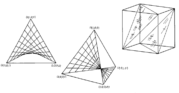
Figure 1: The separable states, or the Segre embedding of ${\mathbb{C}}{\bf P}^{1}\otimes{\mathbb{C}}{\bf P}^{1}$ in ${\mathbb{C}}{\bf P}^{3}$. Two different perspectives of the tetrahedron are given.

There is an interesting relation to the Hopf fibration (see section 3.5) here. Each family of straight lines is also a one parameter family of Hopf circles, and there are two such families because there are two Hopf fibrations, with different twist. We can use our hyperoctant to represent real projective space ${\mathbb{R}}{\bf P}^{3}$, in analogy with Fig. 4.12. The Hopf circles that rule the separable surface are precisely those that get mapped onto each other when we “fold” the hemisphere into a hyperoctant. We now turn to the maximally entangled states, for which the reduced density matrix is the maximally mixed state. Using composite indices we write

$$\rho_{\stackrel{{\scriptstyle\scriptstyle ij}}{{kl}}}=\frac{1}{N}\Gamma_{ij}\Gamma^{*}_{kl}\hskip 14.22636pt\Rightarrow\hskip 14.22636pt{\rho}^{A}_{ik}=\sum_{j=0}^{n}\rho_{\stackrel{{\scriptstyle\scriptstyle ij}}{{kj}}}\ .$$ (16)

Thus

$${\rho}^{A}_{ik}=\frac{1}{N}{\mathbbm{1}}\hskip 14.22636pt\Leftrightarrow\hskip 14.22636pt\sum_{j=0}^{n}\Gamma_{ij}\Gamma^{*}_{kj}={\delta}_{ik}\ .$$ (17)

Therefore the state is maximally entangled if and only if the matrix $\Gamma$ is unitary. Since an overall factor of this matrix is irrelevant for the state we reach the conclusion that the space of maximally entangled states is $SU(N)/{\mathbb{Z}}_{N}$. This happens to be an interesting submanifold of ${\mathbb{C}}{\bf P}^{N^{2}-1}$, because it is at once Lagrangian (a submanifold with vanishing symplectic form and half the dimension of the symplectic embedding space) and minimal (any attempt to move it will increase its volume).

When $N=2$ we are looking at $SU(2)/{\mathbb{Z}}_{2}={\mathbb{R}}{\bf P}^{3}$. To see what this space looks like in the octant picture we observe that

$$\Gamma_{ij}=\left[\begin{array}[]{cc}{\alpha}&{\beta}\\ -{\beta}^{*}&{\alpha}^{*}\end{array}\right]\hskip 14.22636pt\Rightarrow\hskip 14.22636ptZ^{\alpha}=({\alpha},{\beta},-{\beta}^{*},{\alpha}^{*})\ .$$ (18)

In our coordinates this yields three real equations; the space of maximally entangled states will appear in the picture as a straight line connecting two entangled edges and passing through the center of the tetrahedron, while there is a two dimensional surface in the tori. The latter is shifted relative to the separable surface in such a way that the separable and maximally entangled states manage to keep their distance in the torus also when they meet in the octant (at the center of the tetrahedron where the torus is large). Our picture thus displays ${\mathbb{R}}{\bf P}^{3}$ as a one parameter family of two dimensional flat tori, degenerating to circles at the ends of the interval. This is similar to our picture of the 3-sphere, except that this time the lengths of the two intersecting shortest circles on the tori stay constant while the angle between them is changing. It is amusing to convince oneself of the validity of this picture, and to verify that it is really a consequence of the way that the 3-tori are being squashed as we move around the octant.

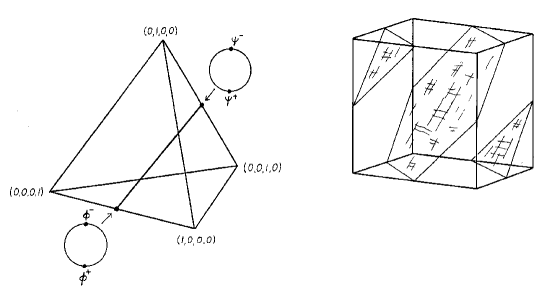
Figure 2: The maximally entangled states form an ${\mathbb{R}}{\bf P}^{3}$, appearing as a straight line in the octant and a surface in the tori. The location of the Bell states is also shown.

As a further illustration we can consider the collapse of a maximally entangled state, say $|{\psi}^{+}\rangle$ for definiteness, when a measurement is performed in laboratory $B$. The result will be a separable state, and because the global state is maximally entangled all the possible outcomes will be equally likely. It is easily confirmed that the possible outcomes form a 2-sphere’s worth of points on the separable surface, distinguished by the fact that they are all lying on the same distance $D_{FS}={\pi}/4$ from the original state. This is the minimal Fubini-Study distance between a separable and a maximally entangled state. The collapse is illustrated in Fig. 3.

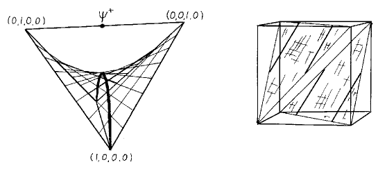
Figure 3: A complete measurement on one of the subsystem will collapse the Bell state $|{\psi}^{+}\rangle$ to a point on a sphere on the separable surface; it appears as a one parameter family of circles in our picture. All points on this sphere are equally likely.

A set of states of intermediate entanglement, quantified by some given value of the Schmidt angle ${\chi}$, is more difficult to draw (although it can be done). For the extreme cases of zero or one e-bit’s worth of entanglement we found the submanifolds ${\mathbb{C}}{\bf P}^{1}\otimes{\mathbb{C}}{\bf P}^{1}$ and $SU(2)/{\mathbb{Z}}_{2}$, respectively. There is a simple reason why these spaces turn up, namely that the amount of entanglement must be left invariant under locally unitary transformations belonging to the group $SU(2)\times SU(2)$. In effect therefore we are looking for orbits of this group, and what we have found are the two obvious possibilities. More generally we will get a stratification of ${\mathbb{C}}{\bf P}^{3}$ into orbits of $SU(2)\otimes SU(2)$; the problem is rather similar to that discussed in section 7.2. Of the exceptional orbits, one is a Kähler manifold and one (the maximally entangled one) is actually a Lagrangian submanifold of ${\mathbb{C}}{\bf P}^{3}$, meaning that the symplectic form vanishes on the latter. A generic orbit will be five real dimensional and the set of such orbits will be labeled by the Schmidt angle ${\chi}$, which is also the minimal distance from a given orbit to the set of separable states. A generic orbit is rather difficult to describe however. Topologically it is a non-trivial fibre bundle with an ${\bf S}^{2}$ as base space and ${\mathbb{R}}{\bf P}^{3}$ as fibre. This can be seen in an elegant way using the Hopf fibration of ${\bf S}^{7}$—the space of normalized state vectors—as ${\bf S}^{4}={\bf S}^{7}/{\bf S}^{3}$; Mosseri and Dandoloff (2001) MD01 provide the details. In the octant picture it appears as a three dimensional volume in the octant and a two dimensional surface in the torus. And with this observation our tour of the two qubit Hilbert space is at an end.

IV Pure states of a bipartite system

Consider a pure state of a composite system $|\psi\rangle\in{\cal H}_{NK}={\cal H}_{N}\otimes{\cal H}_{K}$. The states related by a local unitary transformation,

$$|\psi^{\prime}\rangle\ =\ U\otimes V\,|\psi\rangle\ ,$$ (19)

where $U\in SU(N)$ and $V\in SU(K)$, are called locally equivalent. Sometimes one calls them interconvertible states, since they may be reversibly converted by local transformations one into another JP99 . It is clear that not all pure states are locally equivalent, since the product group $SU(N)\times SU(K)$ forms only a measure zero subgroup of $SU(NK)$. How far can one go from a state using local transformations only? In other words, what is the dimensionality and topology of the orbit generated by local unitary transformations from a given state $|\psi\rangle$?

To find an answer we are going to rely on the Schmidt decomposition (9.8). It consists of not more than $N$ terms, since without loss of generality we have assumed that $K\geq N$. The normalization condition $\langle\psi|\psi\rangle=1$ enforces $\sum_{i=1}^{N}\lambda_{i}=1$, so the Schmidt vector ${\vec{\lambda}}$ lives in the ($N-1$) dimensional simplex $\Delta_{N-1}$. The Schmidt rank of a pure state $|\psi\rangle$ is the number of non–zero Schmidt coefficients, equal to the rank of the reduced state. States with maximal Schmidt rank are generic, and occupy the interior of the simplex, while states of a lower rank live on its boundary.

The Schmidt vector gives the spectra of the partially reduced states, $\rho_{A}={\rm Tr}_{B}(|\psi\rangle\langle\psi|)$ and $\rho_{B}={\rm Tr}_{A}(|\psi\rangle\langle\psi|)$, which differ only by $K-N$ zero eigenvalues. The separable states sit at the corners of the simplex. Maximally entangled states are described by the uniform Schmidt vector, ${\vec{\lambda}}_{*}=\{1/N,\dots,1/N\}$, since the partial trace sends them into the maximally mixed state.

Let ${\vec{\lambda}}=(0,\cdots,0,\kappa_{1},\cdots,\kappa_{1},\kappa_{2},\cdots,\kappa_{2},\dots,\kappa_{J},\cdots,\kappa_{J})$ represent an ordered Schmidt vector, in which each value $\kappa_{n}$ occurs $m_{n}$ times while $m_{0}$ is the number of vanishing coefficients. By definition $\sum_{n=0}^{J}m_{n}=N$, while $m_{0}$ might equal to zero. The local orbit ${\cal O}_{\rm loc}$ generated from $|\psi\rangle$ has the structure of a fibre bundle, in which two quotient spaces

$$\frac{U(N)}{U(m_{0})\times U(m_{1})\times\cdots\times U(m_{J})}{\rm\quad and\quad}\frac{U(N)}{U(m_{0})\times U(1)}$$ (20)

form the base and the fibre, respectively SZK02 . In general such a bundle need not be trivial. The dimensionality of the local orbit may be computed from dimensionalities of the coset spaces,

$${\rm dim}({\cal O}_{\rm loc})=2N^{2}-1-2m_{0}^{2}-\sum_{n=1}^{J}m_{n}^{2}\ .$$ (21)

Table 1: Topological structure of local orbits of the $N\times N$  pure states, $D_{s}$ denotes the dimension of the subspace of the Schmidt simplex $\Delta_{N-1}$, while $D_{o}$ represents the dimension of the local orbit.

$N$	Schmidt coefficients	$D_{s}$	Part of the asymmetric simplex	Local structure: base $\times$ fibre	$D_{o}$
	$(a,b)$	$1$	line	${\bf F}^{(2)}\times{\mathbb{R}}P^{3}$	$5$
$2$	$(1,0)$	$0$	left edge	${\mathbb{C}}{\bf P}^{1}\times{\mathbb{C}}{\bf P}^{1}$	$4$
	$(1/2,1/2)$	$0$	right edge	$U(2)/U(1)={\mathbb{R}}P^{3}$	$3$
	$(a,b,c)$	$2$	interior of triangle	${\bf F}^{(3)}\times\frac{U(3)}{U(1)}$	$14$
	$(a,b,0)$	$1$	base	${\bf F}^{(3)}\times\frac{U(3)}{[U(1)]^{2}}$	$13$
$3$	$(a,b,b)$	$1$	2 upper sides	$\frac{U(3)}{U(1)\times U(2)}\times\frac{U(3)}{U(1)}$	$12$
	$(1/2,1/2,0)$	$0$	right corner	$\frac{U(3)}{U(1)\times U(2)}\times\frac{U(3)}{[U(1)]^{2}}$	$11$
	$(1,0,0)$	$0$	left corner	${\mathbb{C}}{\bf P}^{2}\times{\mathbb{C}}{\bf P}^{2}$	$8$
	$(1/3,1/3,1/3)$	$0$	upper corner	$U(3)/U(1)$	$8$

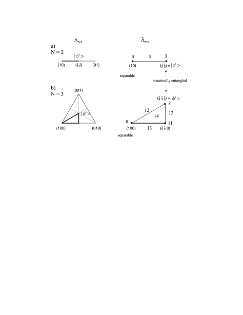
Figure 4: Dimensionality of local orbits generated by a given point of the Weyl chamber $\tilde{\Delta}_{N-1}$ – an asymmetric part of the Schmidt simplex $\Delta_{N-1}$ – for pure states of $N\times N$ problem with $N=2,3$—compare Tab. 1.

Observe that the base describes the orbit of the unitarily similar mixed states of the reduced system $\rho_{A}$, with spectrum $\vec{\lambda}$ and depends on its degeneracy – compare Tab. 8.1. The fibre characterizes the manifold of pure states which are projected by the partial trace to the same density matrix, and depends on the Schmidt rank equal to $N-m_{0}$. To understand this structure consider first a generic state of the maximal Schmidt rank, so that $m_{0}=0$. Acting on $|\psi\rangle$ with $U_{N}\otimes W_{N}$, where both unitary matrices are diagonal, we see that there exist $N$ redundant phases. Since each pure state is determined up to an overall phase, the generic orbit has the local structure

$${\cal O}_{g}\ \approx\ \frac{U(N)}{[U(1)]^{N}}\ \times\ \frac{U(N)}{U(1)}={\bf F}^{(N)}\ \times\ \frac{U(N)}{U(1)},$$ (22)

with dimension ${\rm dim}({\cal O}_{g})=2N^{2}-N-1$. If some of the coefficients are equal, say $m_{J}>1$, then we need to identify all states differing by a block diagonal unitary rotation with $U(m_{J})$ in the right lower corner. In the same way one explains the meaning of the factor $U(m_{0})\times U(m_{1})\times\cdots\times U(m_{J})$ which appears in the first quotient space of (20). If some Schmidt coefficients are equal to zero the action of the second unitary matrix $U_{B}$ is trivial in the $m_{0}$—dimensional subspace—the second quotient space in (20) is $U(N)/[U(m_{0})\times U(1)]$.

For separable states there exists only one non-zero coefficient, $\lambda_{1}=1$, so $m_{0}=N-1$. This gives the Segre embedding (4.16),

$${\cal O}_{\rm sep}=\frac{U(N)}{U(1)\times U(N-1)}\times\frac{U(N)}{U(1)\times U(N-1)}={\mathbb{C}}{\bf P}^{N-1}\times{\mathbb{C}}{\bf P}^{N-1},$$ (23)

of dimensionality ${\rm dim}({\cal O}_{\rm sep})=4(N-1)$. For a maximally entangled state one has $\lambda_{1}=\lambda_{N}=1/N$, hence $m_{1}=N$ and $m_{0}=0$. Therefore

$${\cal O}_{\rm max}=\frac{U(N)}{U(N)}\times\frac{U(N)}{U(1)}=\frac{U(N)}{U(1)}=\frac{SU(N)}{{\mathbb{Z}}_{N}},$$ (24)

with ${\rm dim}({\cal O}_{max})=N^{2}-1$, which equals half the total dimensionality of of the space of pure states.

The set of all orbits foliate ${\mathbb{C}}{\bf P}^{N^{2}-1}$, the space of all pure states of the $N\times N$ system. This foliation is singular, since there exist measure zero leaves of various dimensions and topology. The dimensionalities of all local orbits for $N=2,3$ are shown in Fig. 4, and their topologies in Tab. 1.

Observe that the local orbit defined by (19) contains all purifications of all mixed states acting on ${\cal H}_{N}$ isospectral with $\rho_{N}={\rm Tr}_{K}|\psi\rangle\langle\psi|$. Sometimes one modifies (19) imposing additional restrictions, $K=N$ and $V=U$. Two states fulfilling this strong local equivalence relation (SLE), $|\psi^{\prime}\rangle=U\otimes U|\psi\rangle$ are equal, up to selection of the reference frame used to describe both subsystems. The basis are determined by a unitary $U$. Hence the orbit of the strongly locally equivalent states – the base in (20) – forms a coset space of all states of the form $U\rho_{N}U^{\dagger}$. In particular, for any maximally entangled state, there are no other states satisfying SLE, while for a separable state the orbit of SLE states forms the complex projective space ${\mathbb{C}}{\bf P}^{N-1}$ of all pure states of a single subsystem.

The question, if a given pure state $|\psi\rangle\in{\cal H}_{N}\otimes{\cal H}_{K}$ is separable, is easy to answer: it is enough to compute the partial trace, $\rho_{N}={\rm Tr}_{K}(|\psi\rangle\langle\psi|)$, and to check if ${\rm Tr}\rho_{N}^{2}$ equals unity. If it is so the reduced state is pure, hence the initial pure state is separable. In the opposite case the pure state is entangled. The next question is: to what extent is a given state $|\psi\rangle$ entangled?

There seems not to be a unique answer to this question. Due to the Schmidt decomposition one obtains the Schmidt vector $\vec{\lambda}$ of length $N$ (we assume $N\leq K$), and may describe it by entropies analysed in chapters 2 and 12. For instance, the entanglement entropy is defined as the von Neumann entropy of the reduced state, which is equal to the Shannon entropy of the Schmidt vector,

$$E(|\psi\rangle)\ \equiv\ S(\rho_{A})=S(\vec{\lambda})=-\sum_{i=1}^{N}\lambda_{i}\ln\lambda_{i}\ .$$ (25)

It is equal to zero for separable states and $\ln N$ for maximally entangled states. In the similar way to measure entanglement one may also use the Rényi entropies (2.77) of the reduced state, $E_{q}\equiv S_{q}(\rho_{A})$. We shall need a quantity related to $E_{2}$ called tangle

$$\tau(|\psi\rangle)\ \equiv\ 2(1-{\rm Tr}\rho_{A}^{2})=2\Bigl{(}1-\sum_{i=1}^{N}\lambda_{i}^{2}\Bigr{)}=2\Bigl{(}1-\exp[-E_{2}(|\psi\rangle)]\Bigr{)}\ ,$$ (26)

which runs from $0$ to $2(N-1)/N$, and its square root $C=\sqrt{\tau}$, called concurrence. Concurrence was initially introduced for two qubits by Hill and Wootters HW97 . We adopted here the generalisation of RBCHM01 ; MKB04 , but there are also other ways to generalise this notion for higher dimensions Uh00 ; WC01 ; Woo01 ; AVM01 ; BDHHH02 .

Another entropy, $E_{\infty}=-\ln\lambda_{\rm max}$, has a nice geometric interpretation: if the Schmidt vector is ordered decreasingly and $\lambda_{1}=\lambda_{\rm max}$ denotes its largest component then $|1\rangle\otimes|1\rangle$ is the separable pure state closest to $|\psi\rangle$ LS02 . Thus the Fubini–Study distance of $|\psi\rangle$ to the set of separable pure states, $D_{\rm FS}^{\rm min}=\arccos(\sqrt{\lambda_{\rm max}})$, is a function of $E_{\infty}$. Although one uses several different Rényi entropies $E_{q}$, the entanglement entropy $E=E_{1}$ is distinguished among them just as the Shannon entropy is singled out by its operational meaning discussed in section 2.2.

For the two qubit problem the Schmidt vector has only two components, which sum to unity, so the entropy $E(|\psi\rangle)\in[0,\ln 2]$ characterises uniquely the entanglement of the pure state $|\psi\rangle$. To analyze its geometry it is convenient to select a three dimensional section of the space of pure states - see Fig. 5. The net of this tetrahedron is shown in appendix it presents entanglement at the boundary of the simplex defined by four separable states defining the standard basis.

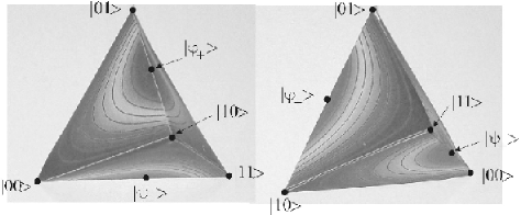
Figure 5: Entropy of entanglement in gray scale for two $3$-D cross-sections of the $6$-D manifold of pure states of two qubits. Both tetrahedrons show the same object from different angles – compare also Figs. 1 and 2.

In general, for an $N\times N$ system the entropy is bounded, $0\leq E\leq\ln N$, and to describe the entanglement completely one needs a set of $N-1$ independent quantities. What properties should they fulfill?

Before discussing this issue we need to distinguish certain classes of quantum operations acting on bipartite systems. Local operations (LO) arise as the tensor product of two maps, both satisfying the trace preserving condition,

$$[\Phi_{A}\otimes\Phi_{B}](\rho)\>=\>\sum_{i}\sum_{j}(A_{i}\otimes B_{j})\,\rho\,(A_{i}^{\dagger}\otimes B_{j}^{\dagger})\ .$$ (27)

Any operation which might be written in the form

$$\Phi_{\rm sep}(\rho)\>=\>\sum_{i}(A_{i}\otimes B_{i})\,\rho\,(A_{i}^{\dagger}\otimes B_{i}^{\dagger})\ ,$$ (28)

is called separable (SO). Observe that this form is more general than (27), even though the summation goes over one index. The third, important class of maps is called LOCC. This name stands for local operations and classical communication and means that all quantum operations, including measurements, are allowed, provided they are performed locally in each subsystem. Classical communication allows the two parties to exchange in both ways classical information about their subsystems, and hence to introduce classical correlations between them. One could think, all separable operations may be obtained in this way, but this is not true BVFMRSSW99 , and we have the proper inclusion relations ${\rm LO}\subset{\rm LOCC}\subset{\rm SO}$.

The concept of local operations leads to the notion of entanglement monotones. These are the quantities which are invariant under unitary operations and decrease, on average, under LOCC Vi00 . The words ’on average’ refer to the general case, in which a pure state is transformed by a probabilistic local operation into a mixture,

$$\rho\ \to\ \sum_{i}p_{i}\rho_{i}\ \ \Rightarrow\ \ \mu(\rho)\ \geq\ \sum_{i}p_{i}\mu(\rho_{i})\ .$$ (29)

Note that if $\mu$ is a non–decreasing monotone, then $-\mu$ is a non–increasing monotone. Thus we may restrict our attention to the non–increasing monotones, which reflect the key paradigm of any entanglement measure: entanglement cannot increase under the action of local operations. Construction of entanglement monotones can be based on

Nielsen’s majorisation theorem Ni99 . A given state $|\psi\rangle$ may be transformed into $|\phi\rangle$ by deterministic LOCC operations if and only if the corresponding vectors of the Schmidt coefficients satisfy the majorisation relation (2.1)

$$|\psi\rangle\>\stackrel{{\scriptstyle\rm LOCC}}{{\longrightarrow}}\>|\phi\rangle\quad\Longleftrightarrow\quad{\vec{\lambda}}_{\psi}\>\prec\>{\vec{\lambda}}_{\phi}.$$ (30)

To prove the forward implication we follow the original proof. Assume that party $A$ performs locally a generalised measurement, which is described by a set of $k$ Kraus operators $A_{i}$. By classical communication the result is sent to party $B$, which performs a local action $\Phi_{i}$, conditioned on the result $i$. Hence

$$\sum_{i=1}^{k}[{\mathbbm{1}}\otimes\Phi_{i}]\bigl{(}A_{i}|\psi\rangle\langle\psi|A_{i}^{\dagger}\bigr{)}=|\phi\rangle\langle\phi|\ .$$ (31)

The result is a pure state so each terms in the sum needs to be proportional to the projector. Tracing out the second subsystem we get

$$A_{i}\rho_{\psi}A_{i}^{\dagger}=p_{i}\rho_{\phi}\ ,\quad\quad i=1,\dots,k,$$ (32)

where $\sum_{i=1}^{k}p_{i}=1$ and $\rho_{\psi}={\rm Tr}_{B}(|\psi\rangle\langle\psi|)$ and $\rho_{\phi}={\rm Tr}_{B}(|\phi\rangle\langle\phi|)$. Due to the polar decomposition of $A_{i}\sqrt{\rho_{\psi}}$ we may write

$$A_{i}\,\sqrt{\rho_{\psi}}=\sqrt{A_{i}\rho_{\psi}A_{i}^{\dagger}}\ V_{i}=\sqrt{p_{i}\rho_{\phi}}\ V_{i}$$ (33)

with unitary $V_{i}$. Making use of the completeness relation we obtain

$$\rho_{\psi}=\sqrt{\rho_{\psi}}\,{\mathbbm{1}}\sqrt{\rho_{\psi}}=\sum_{i=1}^{k}\sqrt{\rho_{\psi}}A_{i}^{\dagger}A_{i}\sqrt{\rho_{\psi}}=\sum_{i=1}^{k}p_{i}V_{i}^{\dagger}\rho_{\phi}V_{i},$$ (34)

and the last equality follows from (33) and its adjoint. Hence we arrived at an unexpected conclusion: if a local transformation $|\psi\rangle\to|\phi\rangle$ is possible, then there exists a bistochastic operation (10.64), which acts on the partially traced states with inversed time - it sends $\rho_{\phi}$ into $\rho_{\psi}$! The quantum HLP lemma (section 2.2) implies the majorisation relation ${\vec{\lambda}}_{\psi}\prec{\vec{\lambda}}_{\phi}$. The backward implication follows from an explicit conversion protocol proposed by Nielsen, or alternative versions presented in Har01 ; JSc01 ; DHR02 .

The majorisation relation (30) introduces a partial order into the set of pure states. (A similar partial order induced by LOCC into the space of mixed states is analysed in HTU01 .) Hence any pure state $|\psi\rangle$ allows one to split the Schmidt simplex, representing the set of all local orbits, into three regions: the set $F$ (Future) contains states which can be produced from $|\psi\rangle$ by LOCC , the set $P$ (Past) of states from which $|\psi\rangle$ may be obtained, and eventually the set $C$ of incomparable states, which cannot be joined by a local transformation in any direction. For $N\geq 4$ there exists an effect of entanglement catalysis JP99 ; DK01 ; BRo02 that allows one to obtain certain incomparable states in the presence of additional entangled states.

This structure resembles the “causal structure” defined by the light cone in special relativity. See Fig. 6, and observe the close similarity to figure 12.2 showing paths in the simplex of eigenvalues that can be generated by bistochastic operations. The only difference is the arrow of time: the ’Past’ for the evolution in the space of density matrices corresponds to the ’Future’ for the local entanglement transformations and vice versa. In both cases the set $C$ of incomparable states contains the same fragments of the simplex $\Delta_{N-1}$. In a typical case $C$ occupies regions close to the boundary of $\Delta_{N-1}$, so one may expect, the larger dimensionality $N$, the larger relative volume of $C$. This is indeed the case, and in the limit $N\to\infty$ two generic pure states of the $N\times N$ system (or two generic density matrices of size $N$) are incomparable CHW02 .

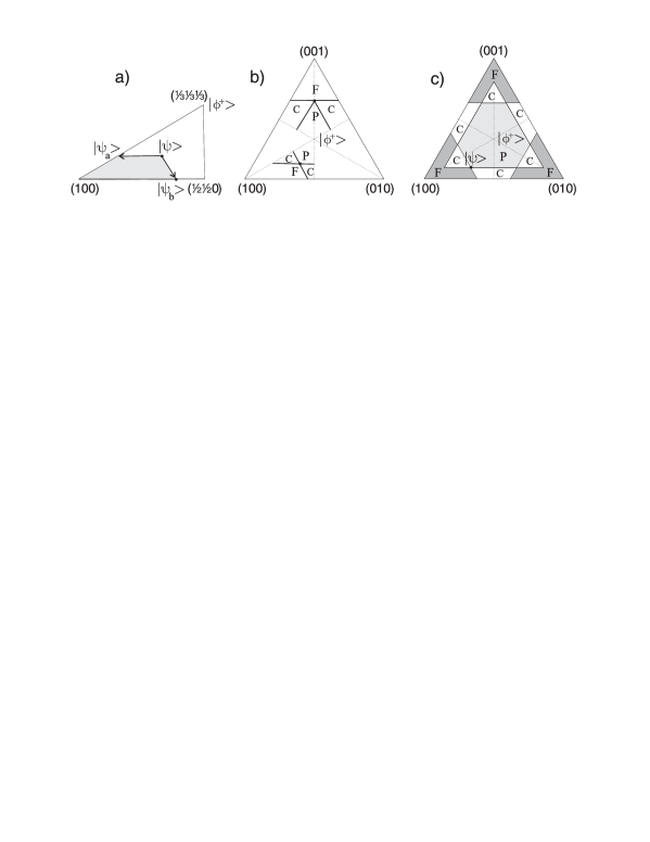
Figure 6: Simplex of Schmidt coefficients $\Delta_{2}$ for $3\times 3$ pure states: the corners represent separable states, center the maximally entangled state $|\phi^{+}\rangle$. Panels (a-c) show ’Future’ and ’Past’ zones with respect to LOCC,

The majorisation relation (30) provides another justification for the observation that two pure states are interconvertible (locally equivalent) if and only if the have the same Schmidt vectors. More importantly, this theorem implies that any Schur concave function of the Schmidt vector $\vec{\lambda}$ is an entanglement monotone. In particular, this crucial property is shared by all Rényi entropies of entanglement $E_{q}(\vec{\lambda})$ including the entanglement entropy (25). To ensure a complete description of a pure state of the $N\times N$ problem one may choose $E_{1},E_{2},\dots,E_{N-1}$. Other families of entanglement monotones include partial sums of Schmidt coefficients ordered decreasingly, $M_{k}(\vec{\lambda})=\sum_{i=1}^{k}\lambda_{k}$ with $k=1,\dots,N-1$ Vi00 , subentropy JRW94 ; MZ03 , and symmetric polynomials in Schmidt coefficients.

Since the maximally entangled state is majorised by all pure states, it cannot be reached from other states by any deterministic local transformation. Is it at all possible to create it locally? A possible clue is hidden in the word average contained in the majorisation theorem.

Let us assume we have at our disposal $n$ copies of a generic pure state $|\psi\rangle$. The majorisation theorem does not forbid us to locally create out of them $m$ maximally entangled states $|\psi^{+}\rangle$, at the expense of the remaining $n-m$ states becoming separable. Such protocols proposed in BBPS96 ; LP01 are called entanglement concentration. This local operation is reversible, and the reverse process of transforming $m$ maximally entangled states and $n-m$ separable states into $n$ entangled states is called entanglement dilution. The asymptotic ratio $m/n\leq 1$ obtained by an optimal concentration protocol is called distillable entanglement BBPS96 of the state $|\psi\rangle$.

Assume now that only one copy of an entangled state $|\psi\rangle$ is at our disposal. To generate maximally entangled state locally we may proceed in a probabilistic way: a local operation produces $|\psi^{+}\rangle$ with probability $p$ and a separable state otherwise. Hence we allow a pure state $|\psi\rangle$ to be transformed into a mixed state. Consider a probabilistic scheme to convert a pure state $|{\psi}\rangle$ into a target $|\phi\rangle$ with probability $p$. Let $p_{c}$ be the maximal number such that the following majorisation relation holds,

$$\lambda_{\psi}\ \prec\ p_{c}\,\vec{\lambda}_{\phi}.$$ (35)

It is easy to check that the probability $p$ cannot be larger than $p_{c}$, since the Nielsen theorem would be violated. The optimal conversion strategy for which $p=p_{c}$ was explicitly constructed by Vidal Vi99 . The Schmidt rank cannot increase during any local conversion scheme LP01 . If the rank of the target state $|\phi\rangle$ is larger than the Schmidt rank of $|{\psi}\rangle$, then $p_{c}=0$ and the probabilistic conversion cannot be performed. In such a case one may still perform a faithful conversion JP99a ; VJN00 transforming the initial state $|\psi\rangle$ into a state $|\phi^{\prime}\rangle$, for which its fidelity with the target, $|\langle\phi|\phi^{\prime}\rangle|^{2}$, is maximal.

This situation is illustrated in Fig. 7, which shows the probability of accessing different regions of the Schmidt simplex for pure states of a $3\times 3$ system for four different initial states $|\psi\rangle$. The shape of the black figure ($p=1$ represents deterministic transformations) is identical with the set ’Future’ in Fig. 6. The more entangled final state $|\phi\rangle$ (closer to the maximally entangled state – black $(*)$ in the center of the triangle), the smaller probability $p$ of a successful transformation. Observe that the contour lines (plotted at $p=0.2,0.4,0.6$ and $0.8$) are constructed from the iso-entropy lines $S_{q}$ for $q\to 0$ and $q\to\infty$,

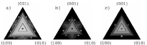
Figure 7: Probability of the optimal local conversion of an initial state $|\psi\rangle$ (white $\times$) of the $3\times 3$ problem into a given pure state represented by a point in the Schmidt simplex. Initial Schmidt vector $\vec{\lambda}_{\psi}$ is (a) $(0.7,0.25,0.05)$, (b) $(0.6,0.27,0.03)$, and (c) $(0.8,0.1,0.1)$. Due to the degeneracy of $\vec{\lambda}$ in the latter case there exist only three interconvertible states in $\Delta_{2}$, represented by $(+)$.

Let us close with an envoi: entanglement of a pure state of any bipartite system may be fully characterized by its Schmidt decomposition. In particular, all entanglement monotones are functions of the Schmidt coefficients. However, the Schmidt decomposition cannot be directly applied to the multi–partite case Pe95 ; CHS00 ; AAJ01 . These systems are still being investigated - several families of local invariants and entanglement monotones were found Su00 ; BC01 ; Gi02 , properties of local orbits were analysed MD01 ; BC03 ; Mi03 ; Le04b , measures of multi–partite entanglement were introduced CKW00 ; BPRST01 ; WC01 ; MW02 ; Br03 ; HBj04 , and a link between quantum mechanical and topological entanglement including knots and braids KL02 ; AKMR04 , rings OW01 , and graphs PB03 ; HEB04 has been discussed. Let us just mention that pure states of three qubits can be entangled in two inequivalent ways. There exist three-qubit pure states GHZ89

$$|GHZ\rangle=\frac{1}{\sqrt{2}}\bigl{(}|000\rangle+|111\rangle\bigr{)}{\quad\rm and\quad}|W\rangle=\frac{1}{\sqrt{3}}\bigl{(}|001\rangle+|010\rangle+|100\rangle\bigr{)}\,$$ (36)

which cannot be locally converted with a positive probability in any direction DVC00 . A curious reader might be pleased to learn that four qubits can be entangled in nine different ways VDDV02 . What is the number of different ways, one may entangle $m$ qubits?

V Mixed states and separability

It is a good time to look again at mixed states: in this section we shall analyze bipartite density matrices, acting on a composite Hilbert space ${\cal H}={\cal H}_{A}\otimes{\cal H}_{B}$ of finite dimensionality $d=NK$. A state is called a product state, if it has a tensor product structure, $\rho=\rho_{A}\otimes\rho_{B}$. A mixed state $\rho$ is called separable, if it can be represented as a convex sum of product states We89 ,

$$\rho_{sep}\>=\>\sum_{j=1}^{M}\,q_{j}\,\rho^{A}_{j}\otimes\rho^{B}_{j}\ ,$$ (37)

where $\rho^{A}$ acts in ${\cal H}_{A}$ and $\rho^{B}$ acts in ${\cal H}_{B}$, the weights are positive, $q_{j}>0$, and sum to unity, $\sum_{j=1}^{M}q_{j}=1$. Such a decomposition is not unique. For any separable $\rho$, the smallest number $M$ of terms is called cardinality  of the state. Due to Carathéodory’s theorem the cardinality is not larger then $d^{2}$ Ho97 . In the two–qubit case it is not larger than $d=4$ STV98 , while for systems of higher dimensions it is typically larger than the rank $r\leq d$ Lo00 .

By definition the set ${\cal M}_{S}$ of separable mixed states is convex. Separable states can be constructed locally using classical communication, and may exhibit classical correlations only. A mixed state which is not separable, hence may display non–classical correlations, is called entangled. It is easy to see that for pure states both definitions are consistent. The notion of entanglement may also be used in the set-up of classical probability distributions Tu00 , theory of Lie-algebras or convex sets BKOV03 and may be compared with secret classical correlations CP02 .

Any density matrix $\rho$ acting on $d$ dimensional Hilbert space may be represented as a sum (8.10) over $d^{2}-1$ trace-less generators $\sigma_{i}$ of $SU(d)$. However, analysing a composite system for which $d=NK$, it is more advantageous to use the basis of the product group $SU(N)\otimes SU(K)$, which leads us to the Fano form Fa83

$$\rho=\frac{1}{NK}\Bigl{[}{\mathbbm{1}}_{NK}+\!\sum_{i=1}^{N^{2}-1}\tau^{A}_{i}\sigma_{i}\otimes{\mathbbm{1}}_{K}+\!\sum_{j=1}^{K^{2}-1}\tau^{B}_{j}{\mathbbm{1}}_{N}\otimes\sigma_{j}+\!\sum_{i=1}^{N^{2}-1}\sum_{j=1}^{K^{2}-1}\beta_{ij}\sigma_{i}\otimes\sigma_{j}\Bigr{]}\ .$$ (38)

Here $\vec{\tau}^{A}$ and $\vec{\tau}^{B}$ are Bloch vectors of the partially reduced states, while a real $(N^{2}-1)\times(K^{2}-1)$ matrix $\beta$ describes the correlation between both subsystems. If $\beta=0$ then the state is separable, but the reverse is not true. Note that for product states $M_{ij}\equiv\beta_{ij}-\tau^{A}_{i}\tau^{B}_{j}=0$, hence the norm $||M||^{2}$ characterises to what extent $\rho$ is not a product state SM95 . Keeping both Bloch vectors constant and varying $\beta$ in such a way to preserve positivity of $\rho$ we obtain a $(N^{2}-1)(K^{2}-1)$ dimensional family of bi-partite mixed states, which are locally indistinguishable.

The definition of separability (37) is implicit, so it is in general not easy to see, if such a decomposition exists for a given density matrix. Separability criteria found so far may be divided into two disjoint classes: A) sufficient and necessary, but not practically usable; and B) easy to use, but only necessary (or only sufficient). A simple, albeit amazingly powerful criterion was found by Peres Pe96 , who analyzed the action of partial transposition on an arbitrary separable state,

$$\rho_{\rm sep}^{T_{A}}\ \equiv\ (T\otimes{\mathbbm{1}})(\rho_{\rm sep})=\sum_{j}\,q_{j}\,(\rho^{A}_{j})^{T}\otimes\rho^{B}_{j}\geq 0.$$ (39)

Thus any separable state has a positive partial transpose (is PPT), so we obtain directly

B1. PPT criterion. If $\rho^{T_{A}}\not\geq 0$, the state $\rho$ is entangled.

Is is extremely easy to use: all we need to do is to perform the partial transposition of the density matrix in question, diagonalise, and check if all eigenvalues are non–negative. Although partial transpositions were already defined in (10.28), let us have a look, how both operations act on a block matrix,

$$X=\left[\begin{array}[]{c c}A&B\\ C&D\end{array}\right],\quad X^{T_{B}}\equiv\left[\begin{array}[]{c c}A^{T}&B^{T}\\ C^{T}&D^{T}\end{array}\right]\ ,\quad X^{T_{A}}\equiv\left[\begin{array}[]{c c}A&C\\ B&D\end{array}\right]\ .$$ (40)

Note that $X^{T_{B}}=(X^{T_{A}})^{T}$, so the spectra of the two operators are the same and the above criterion may be equivalently formulated with the map $T_{B}=({\mathbbm{1}}\otimes T)$. Furthermore, partial transposition applied on a density matrix produces the same spectrum as the transformation of flipping one of both Bloch vectors present in its Fano form (38). Alternatively one may change the signs of all generators $\sigma_{j}$ of the corresponding group. For instance, flipping the second of the two subsystems of the same size we obtain

$$\rho^{F_{B}}\equiv\frac{1}{N^{2}}\Bigl{[}{\mathbbm{1}}_{N^{2}}+\sum_{i=1}^{N^{2}-1}\tau^{A}_{i}\sigma_{i}\otimes{\mathbbm{1}}_{N}-\sum_{j=1}^{N^{2}-1}\tau^{B}_{j}{\mathbbm{1}}_{N}\otimes\sigma_{j}-\sum_{i,j=1}^{N^{2}-1}\beta_{ij}\sigma_{i}\otimes\sigma_{j}\Bigr{]}\ ,$$ (41)

with the same spectrum as $\rho^{T_{A}}$ and $\rho^{T_{B}}$. In the two–qubit case, reflection of all three components of the Bloch vector, ${\vec{\tau}}^{B}\to-{\vec{\tau}}^{B}$, is equivalent to changing the sign of its single component $\tau^{B}_{y}$ (partial transpose), followed by the $\pi$–rotation along the $y$–axis.

To watch the PPT criterion in action consider the family of generalised Werner states  which interpolate between maximally mixed state $\rho_{*}$ and the maximally entangled state $P_{+}=|\phi^{+}\rangle\langle\phi^{+}|$, (For the original Werner states We89 the singlet pure state $|\psi^{-}\rangle=(|01\rangle-|10\rangle)/\sqrt{2}$ was used instead of $|\phi^{+}\rangle$),

$$\rho_{W}(x)=x|\phi^{+}\rangle\langle\phi^{+}|+(1-x)\frac{1}{N}{\mathbbm{1}}{\rm\quad with\quad}x\in[0,1]\ .$$ (42)

One eigenvalue equals $[1+(N-1)x]/N$, and the remaining $(N-1)$ eigenvalues are degenerate and equal to $(1-x)/N$. In the $N=2$ case:

$$\rho_{x}=\frac{1}{4}\left[\begin{array}[]{c c c c}1+x&0&0&2x\\ 0&1-x&0&0\\ 0&0&1-x&0\\ 2x&0&0&1+x\end{array}\right],\quad\rho_{x}^{T_{A}}=\frac{1}{4}\left[\begin{array}[]{c c c c}1+x&0&0&0\\ 0&1-x&2x&0\\ 0&2x&1-x&0\\ 0&0&0&1+x\end{array}\right].$$ (43)

Diagonalisation of the partially transposed matrix $\rho_{x}^{T_{A}}=\rho_{x}^{T_{B}}$ gives the spectrum $\frac{1}{4}\{1+x,1+x,1+x,1-3x\}$. This matrix is positive definite if $x\leq 1/3$, hence Werner states are entangled for $x>1/3$. It is interesting to observe that the critical state $\rho_{1/3}\in\partial{\cal M}_{\rm sep}$, is localized at the distance $r_{\rm in}=1/\sqrt{24}$ from the maximally mixed state $\rho_{*}$, so it sits on the insphere, the maximal sphere that one can inscribe into the set ${\cal M}^{(4)}$ of $N=4$ mixed states.

As we shall see below the PPT criterion works in both direction only if dim$({\cal H})\leq 6$, so there is a need for other separability criteria LBCKKSST00 ; HHH00b ; BCHHKLS02 ; Te02 ; Br02 . Before reviewing the most important of them let us introduce one more notion often used in the physical literature.

An Hermitian operator $W$ is called an entanglement witness for a given entangled state $\rho$ if Tr$\rho W<0$ and Tr$\rho\sigma\geq 0$ for all separable $\sigma$ HHH96a ; Te00 . For convenience the normalisation Tr$W=1$ is assumed. Horodeccy HHH96a proved a useful

Witness lemma. For any entangled state $\rho$ there exists an entanglement witness $W$.

In fact this is the Hahn-Banach separation theorem (section 1.1) in slight disguise.

It is instructive to realise a direct relation with the dual cones construction discussed in chapter 11: any witness operator is proportional to a dynamical matrix, $W=D_{\Phi}/N$, corresponding to a non-completely positive map $\Phi$. Since $D_{\Phi}$ is block positive (positive on product states), the condition Tr$\,W\sigma\geq 0$ holds for all separable states for which the decomposition (37) exists. Conversely, a state $\rho$ is separable if Tr$\,W\rho\geq 0$ for all block positive $W$. This is just the definition (11.15) of a super-positive map $\Psi$. We arrive, therefore, at a key observation: the set ${\cal SP}$ of super-positive maps is isomorphic with the set ${\cal M}_{S}$ of separable states by the Jamiołkowski isomorphism, $\rho=D_{\Psi}/N$.

An intricate link between positive maps and the separability problem is made clear in the

A1. Positive maps criterion HHH96a . A state $\rho$ is separable if and only if $\rho^{\prime}=(\Phi\otimes{\mathbbm{1}})\rho$ is positive for all positive maps $\Phi$.

To demonstrate that this condition is necessary, act with an extended map on the separable state (37),

$$\Bigl{(}\Phi\otimes{\mathbbm{1}}\Bigr{)}\Bigl{(}\sum_{j}q_{j}\,\rho^{A}_{j}\otimes\rho^{B}_{j}\Bigr{)}\>=\>\sum_{j}q_{j}\,\Phi(\rho^{A}_{j})\otimes\rho^{B}_{j}\>\geq\>0\>.$$ (44)

Due to positivity of $\Phi$ the above combination of positive operators is positive. To prove sufficiency, assume that $\rho^{\prime}=(\Phi\otimes{\mathbbm{1}})\rho$ is positive. Thus Tr$\rho^{\prime}P\geq 0$ for any projector $P$. Setting $P=P_{+}=|\phi^{+}\rangle\langle\phi^{+}|$ and making use of the adjoint map we get Tr$\rho(\Phi\otimes{\mathbbm{1}})P_{+}=\rm\frac{1}{N}{Tr}\rho D_{\Phi}\geq 0$. Since this property holds for all positive maps $\Phi$, it implies separability of $\rho$ due to the witness lemma $\square$.

The positive maps criterion holds also if the map acts on the second subsystem. However, this criterion is not easy to use: one needs to verify that the required inequality is satisfied for all positive maps. The situation becomes simple for the $2\times 2$ and $2\times 3$ systems. In this case any positive map is decomposable due to the Størmer–Woronowicz theorem and may be written as a convex combination of a CP map and a CcP map, which involves the transposition $T$ (see section 11.1). Hence, to apply the above criterion we need to perform one check working with the partial transposition $T_{A}=(T\otimes{\mathbbm{1}})$. In this way we become

B1’. Peres–Horodeccy criterion Per96 ; HHH96a . A state $\rho$ acting on ${\cal H}_{2}\otimes{\cal H}_{2}$ (or ${\cal H}_{2}\otimes{\cal H}_{3}$) composite Hilbert space is separable if and only if $\rho^{T_{A}}\geq 0$.

In general, the set of bi–partite states may be divided into PPT states (positive partial transpose) and NPPT states (not PPT). A map $\Phi$ is related by the Jamiołkowski isomorphism to a PPT state if $\Phi\in{\cal CP}\cap{\cal C}c{\cal P}$. Complete co–positivity of $\Phi$ implies that $T\Phi$ is completely positive, so $(T\Phi\otimes{\mathbbm{1}})\rho\geq 0$ for any state $\rho$. Thus $\rho^{\prime}=(\Phi\otimes{\mathbbm{1}})\rho$, is a PPT state, so such a map may be called PPT–inducing, ${\cal PPTM}\equiv{\cal CP}\cap{\cal C}c{\cal P}$. These maps should not be confused with PPT–preserving maps Ra01 ; EVWW01 , which act on bi–partite systems and fulfill another property: if $\rho^{T_{A}}\geq 0$ then $(\Psi(\rho))^{T_{A}}\geq 0$.

Similarly, a super-positive map $\Phi$ is related by the isomorphism (11.22) with a separable state. Hence $(\Phi\otimes{\mathbbm{1}})$ acting on the maximally entangled state $|\phi^{+}\rangle\langle\phi^{+}|$ is separable. It is then not surprising that $\rho^{\prime}=(\Phi\otimes{\mathbbm{1}})\rho$ becomes separable for an arbitrary state $\rho$ HSR03 , which explains why SP maps are also called entanglement breaking channels. Furthermore, due to the positive maps criterion $(\Psi\otimes{\mathbbm{1}})\rho^{\prime}\geq 0$ for any positive map $\Psi$. In this way we have arrived at the first of three duality conditions equivalent to (11.16-11.18),

$$\{\Phi\in{\cal SP}\}\ \ \Leftrightarrow\ \ \Psi\cdot\Phi\in{\cal CP} {\rm\quad for\quad all\quad}\Psi\in{\cal P}\ ,$$ (45)

$$\{\Phi\in{\cal CP}\}\ \ \Leftrightarrow\ \ \Psi\cdot\Phi\in{\cal CP} {\rm\quad for\quad all\quad}\Psi\in{\cal CP}\ ,$$ (46)

$$\{\Phi\in{\cal P}\}\ \ \Leftrightarrow\ \ \Psi\cdot\Phi\in{\cal CP} {\rm\quad for\quad all\quad}\Psi\in{\cal SP}\ .$$ (47)

The second one reflects the fact that a composition of two CP maps is CP, while the third one is dual to the first.

Due to the Størmer and Woronowicz theorem and the Peres–Horodeccy criterion, all PPT states for $2\times 2$ and $2\times 3$ problems are separable (hence any PPT-inducing map is SP) while all NPPT states are entangled. In higher dimensions there exist PPT entangled states (PPTES), and this fact motivates investigation of positive, non–decomposable maps and other separability criteria.

B2. Range criterion Ho97 . If a state $\rho$ is separable, then there exists a set of pure product states such that $|\psi_{i}\otimes\phi_{i}\rangle$ span the range of $\rho$ and $T_{B}(|\psi_{i}\otimes\phi_{i}\rangle$ span the range of $\rho^{T_{B}}$.

The action of the partial transposition on a product state gives $|\psi_{i}\otimes\phi_{i}^{*}\rangle$, where ^∗ denotes complex conjugation in the standard basis. This criterion, proved by P. Horodecki Ho97 , allowed him to identify the first PPTES in the $2\otimes 4$ system. Entanglement of $\rho$ was detected by showing that none of the product states from the range of $\rho$, if partially conjugated, belong to the range of $\rho^{T_{B}}$.

The range criterion allows one to construct PPT entangled states related to unextendible product basis, (UPB). It is a set of orthogonal product vectors $|u_{i}\rangle\in{\cal H}_{N}\otimes{\cal H}_{M}$, $i=1,\dots,k<MN$, such that there does not exist any product vectors orthogonal to all of them BVMSST99 ; AL01 ; VMSST03 . We shall recall an example found in BVMSST99 for $3\times 3$ system,

$$|u_{1}\rangle = \frac{1}{\sqrt{2}}|0\rangle\otimes|0-1\rangle,\quad|u_{2}\rangle=\frac{1}{\sqrt{2}}|2\rangle\otimes|1-2\rangle,\quad|u_{3}\rangle=\frac{1}{\sqrt{2}}|0-1\rangle\otimes|2\rangle,$$

$$|u_{4}\rangle = \frac{1}{\sqrt{2}}|1-2\rangle\otimes|0\rangle,\quad|u_{5}\rangle=\frac{1}{3}|0+1+2\rangle\otimes|0+1+2\rangle.$$ (48)

These five states are mutually orthogonal. However, since they span full three dimensional spaces in both subsystems, no product state may be orthogonal to all of them.

For a given UPB let $P=\sum_{i=1}^{k}|u_{i}\rangle\langle u_{i}|$ denote the projector on the space spanned by these product vectors. Consider the mixed state, uniformly covering the complementary subspace,

$$\rho\ \equiv\ \frac{1}{MN-k}\ ({\mathbbm{1}}-P)\ .$$ (49)

By construction this subspace does not contain any product vectors, so $\rho$ is entangled due to the range criterion. On the other hand, the projectors $(|u_{i}\rangle\langle u_{i}|)^{T_{B}}$ are mutually orthogonal, so the operator $P^{T_{B}}=\sum_{i=1}^{k}(|u_{i}\rangle\langle u_{i}|)^{T_{B}}$ is a projector. So is $({\mathbbm{1}}-P)^{T_{B}}$, hence $\rho^{T_{B}}$ is positive. Thus the state (49) is a positive partial transpose entangled state. The UPB method was used to construct PPTES in BVMSST99 ; BP00 ; VMSST03 ; Pi04 , while not completely positive maps were applied in HKP03 ; BFP04 for this purpose. Conversely, PPTES were used in Te00 to find non-decomposable positive maps.

B3. Reduction criterion CAG99 ; HH99 . If a state $\rho$ is separable then the reduced states $\rho_{A}={\rm Tr}_{B}\rho$ and $\rho_{B}={\rm Tr}_{A}\rho$ satisfy

$$\rho_{A}\otimes{\mathbbm{1}}-\rho\geq 0{\quad\rm and\quad}{\mathbbm{1}}\otimes\rho_{B}-\rho\geq 0\ .$$ (50)

This statement follows directly from the positive maps criterion with the map $\Phi(\sigma)=({\rm Tr}\sigma){\mathbbm{1}}-\sigma$ applied to the first or the second subsystem. Computing the dynamical matrix for this map composed with the transposition, $\Phi^{\prime}=\Phi T$, we find that $D_{\Phi^{\prime}}\geq 0$, hence $\Phi$ is CcP and (trivially) decomposable. Thus the reduction criterion cannot be stronger than the PPT criterion (which is the case for the generalised reduction criterion ACF03 ).

There exists, however, a good reason to pay some attention to the reduction criterion: the Horodeccy brothers have shown HH99 that any state $\rho$ violating (50) is distillable, i.e. there exists a LOCC protocol which allows one to extract locally maximally entangled states out of $\rho$ or its copies BVSW96 ; Ra99b . Entangled states, which are not distillable are called bound entangled HHH98 ; HHH99 .

A general question, which mixed state may be distilled is not solved yet BCHHKLS02 . (Following literature we use two similar terms: entanglement concentration and distillation, for local operations performed on pure and mixed states, respectively. While the former operations are reversible, the latter are not.) Again the situation is clear for systems with dim$({\cal H})\leq 6$: all PPT states are separable, and all NPPT states are entangled and distillable. For larger systems there exists PPT entangled states and all of them are not distillable, hence bound entangled HHH98 . (Interestingly, there are no bound entangled states of rank one nor two HSTT03 .) Conversely, one could think that all NPPT entangled states are distillable, but this seems not to be the case DCLB00 ; VSSTT00 .

B4. Majorisation criterion NK01 . If a state $\rho$ is separable, then the reduced states $\rho_{A}$ and $\rho_{B}$ satisfy the majorisation relations

$$\rho\prec\rho_{A}{\rm\quad\quad and\quad\quad}\rho\prec\rho_{B}\ .$$ (51)

In brief, separable states are more disordered globally than locally. To prove this criterion one needs to find a bistochastic matrix $B$ such that the spectra satisfy ${\vec{\lambda}}=B{\vec{\lambda}_{A}}$. The majorisation relation implies that any Schur convex functions satisfies the inequality (2.8). For Schur concave functions the direction of the inequality changes. In particular, the

B5. Entropy criterion. If a state $\rho$ is separable, then the Rényi entropies fulfill

$$S_{q}(\rho)\geq S_{q}(\rho_{A}){\rm\quad and\quad}S_{q}(\rho)\geq S_{q}(\rho_{B}){\quad\rm for\quad}q\geq 0\ ,$$ (52)

follows. The entropy criterion was originally formulated for $q=1$ HH94 . Then this statement may be equivalently expressed in terms of the conditional entropy, $S(A|B)=S(\rho_{AB})-S(\rho_{A})$: for any separable bi-partite state $S(A|B)$ is non–negative. (The opposite quantity, $-S(A|B)$, is called coherent quantum information SN96 and plays an important role in quantum communication HHHO05 .)

Thus negative conditional entropy of a state $\rho_{AB}$ confirms its entanglement HH96 ; SN96 ; CA99 . The entropy criterion was proved for $q=2$ in HHH96b and later formulated also for the Havrda–Charvat–Tsallis entropy (2.77) AR01 ; TLB01 ; RR02 ; RC02 . Its combination with the entropic uncertainty relations of Massen and Uffink MU88 provides yet another interesting family of separability criteria GL04 . However, it is worth to emphasize that in general the spectral properties do not determine separability—there exist pairs of isospectral states, one of which is separable, the other not.

A2. Contraction criterion. A bi-partite state $\rho$ is separable if and only if any extended trace preserving positive map act as a (weak) contraction in sense of the trace norm,

$$||\rho^{\prime}||_{\rm Tr}\>=\>||({\mathbbm{1}}\otimes\Phi)\rho||_{\rm Tr}\>\leq\>||\rho||_{\rm Tr}\>=\>{\rm Tr}\rho\>=\>1\ .$$ (53)

This criterion was formulated in HHH02 basing on earlier papers Rud02 ; CW03 . To prove it notice that the sufficiency follows from the positive map criterion: since Tr$\rho^{\prime}=1$, hence $||\rho^{\prime}||_{\rm Tr}\leq 1$ implies that $\rho^{\prime}\geq 0$. To show the converse consider a normalised product state $\rho=\rho^{A}\otimes\rho^{B}$. Any trace preserving positive map $\Phi$ acts as isometry in sense of the trace norm, and the same is true for the extended map,

$$||\rho^{\prime}||_{\rm Tr}=\bigl{|}\bigr{|}({\mathbbm{1}}\otimes\Phi)(\rho^{A}\otimes\rho^{B})\bigl{|}\bigr{|}_{\rm Tr}=||\rho^{A}||\cdot||\Phi(\rho^{B})||_{\rm Tr}=1\ .$$ (54)

Since the trace norm is convex, $||A+B||_{\rm Tr}\leq||A||_{\rm Tr}+||B||_{\rm Tr}$, any separable state fulfills

$$\Bigl{|}\Bigr{|}({\mathbbm{1}}\otimes\Phi)\Bigl{(}\sum_{i}q_{i}(\rho^{A}_{i}\otimes\rho^{B}_{i})\Bigr{)}\Bigl{|}\Bigr{|}_{\rm Tr}\ \leq\ \sum_{i}q_{i}\,||\rho^{A}_{i}\otimes\Phi(\rho^{B}_{i})||_{\rm Tr}\ =\ \sum_{i}q_{i}=1\ ,$$ (55)

which ends the proof. $\square$.

Several particular cases of this criterion could be useful. Note that the celebrated PPT criterion B1 follows directly, if the transposition $T$ is selected as a trace preserving map $\Phi$, since the norm condition, $||\rho^{T_{A}}||_{\rm Tr}\leq 1$, implies positivity, $\rho^{T_{A}}\geq 0$. Moreover, one may formulate an analogous criterion for global maps $\Psi$, which act as contractions on any bi–partite product states, $||\Psi(\rho_{A}\otimes\rho_{B})||_{\rm Tr}\leq 1$. As a representative example let us mention

B6. Reshuffling criterion. (also called also realignement criterion CW03 or computable cross-norm criterion Rud03 ). If a bi-partite state $\rho$ is separable then reshuffling (10.33) does not increase its trace norm,

$$||\rho^{R}||_{\rm Tr}\ \leq\ ||\rho||_{\rm Tr}=1\ .$$ (56)

We shall start the proof considering an arbitrary product state, $\sigma_{A}\otimes\sigma_{B}$. By construction its Schmidt decomposition consists of one term only. This implies

$$||(\sigma_{A}\otimes\sigma_{B})^{R}||_{\rm Tr}=2\,||\sigma_{A}||_{2}\cdot||\sigma_{B}||_{2}=\sqrt{{\rm Tr}\,\sigma_{A}^{2}}\,\sqrt{{\rm Tr}\,\sigma_{B}^{2}}\ \leq\ 1\ .$$ (57)

Since the reshuffling transformation is linear, $(A+B)^{R}=A^{R}+B^{R}$, and the trace norm is convex, any separable state satisfies

$$\Bigl{|}\Bigr{|}\Bigl{(}\sum_{i}q_{i}(\sigma^{A}_{i}\otimes\sigma^{B}_{i})\Bigr{)}^{R}\Bigl{|}\Bigr{|}_{\rm Tr}\ \leq\ \sum_{i}q_{i}||(\sigma^{A}_{i}\otimes\sigma^{B}_{i})^{R}||_{\rm Tr}\ \leq\ \sum_{i}q_{i}=1\ ,$$ (58)

which completes the reasoning. $\square$.

In the simplest case of two qubits, the latter criterion is weaker than the PPT: examples of NPPT states, the entanglement of which is not detected by reshuffling, were provided by Rudolph Rud03 . However, for some larger dimensional problems the reshuffling criterion becomes useful, since it is capable of detecting PPT entangled states, for which $||\rho^{R}||_{\rm Tr}>1$ CW03 .

There exists several other separability criteria, not discussed here. Let us mention applications of the range criterion for $2\times N$ systems DCLB00 , checks for low rank density matrices HLVC00 , reduction of the dimensionality of the problem Woe04 , relation between purity of a state and its maximal projection on a pure states LBCKKSST00 , or criterion obtained by expanding a mixed state in the Fourier basis PR00 . The problem which separability criterion is the strongest, and what the implication chains among them are, remains a subject of a vivid research VW02 ; ACF03 ; CW04 ; BPCP04 . In general, the separability problem is ’hard’, since it is known that it belongs to the NP complexity class Gu03 . Due to this intriguing mathematical result it is not surprising that all operationally feasible analytic criteria provide partial solutions only. On the other hand, one should appreciate practical methods constructed to decide separability numerically. Iterative algorithms based on an extension of the PPT criterion for higher dimensional spaces DPS02 ; DPS04 or non-convex optimization EHGC04 are able to detect the entanglement in a finite number of steps. Another algorithm provides an explicit decomposition into pure product states HBr04 , confirming that the given mixed state $\rho$ is separable. A combination of these two approaches terminates after a finite time $t$ and gives an inconclusive answer only if $\rho$ belongs to the $\epsilon$–vicinity of the boundary of the set of separable states. By increasing the computation time $t$ one may make the width $\epsilon$ of the ’no–man’s land’ arbitrarily small.

VI Geometry of the set of separable states

Equipped with a broad spectrum of separability criteria, we may try to describe the structure of the set ${\cal M}_{S}$ of the separable states. This task becomes easier for the two–qubit system, for which positive partial transpose implies separability. Hence the set of $N=4$ separable states arises as an intersection of the entire body of mixed states with its reflection induced by partial transpose,

$${\cal M}^{(4)}_{S}={\cal M}^{(4)}\ \cap\ T_{A}({\cal M}^{(4)})\$$ (59)

This observation suggests that the set of separable states has a positive volume. The maximally mixed state is invariant with respect to partial transpose, $\rho_{*}=\rho_{*}^{T_{B}}$ and occupies the center of the body ${\cal M}^{(4)}$. It is thus natural to ask, what is the radius of the separable ball centered at $\rho_{*}$? The answer its very appealing in the simplest, Euclidean geometry: the entire maximal $15$-D ball inscribed in ${\cal M}^{(4)}$ is separable ZHSL98 . Working with the distance $D_{2}$ defined in eq. (9.26), its radius reads $r_{\rm in}=1/\sqrt{24}$.

The separable ball is sketched in two or three dimensional cross–sections of ${\cal M}^{(4)}$ in Fig. 8. To prove its separability we shall invoke

Mehta’s Lemma Me89 . Let $A$ be a Hermitian matrix of size $D$ and let $\alpha={\rm Tr}A/\sqrt{{\rm Tr}A^{2}}$. If $\alpha\geq\sqrt{D-1}$ then $A$ is positive.

Its proof begins with an observation that both traces are basis independent, so we may work in the eigenbasis of $A$. Let $(x_{1},\dots x_{D})$ denote the spectrum of $A$. Assume first that one eigenvalue, say $x_{1}$, is negative. Making use of the right hand side of the standard estimation between the ${l}_{1}$ and ${l}_{2}$–norms (with prefactor $1$) of an $N$–vector, $||A||_{2}\leq||A||_{1}\leq N||A||_{2}$, we infer

$${\rm TrA}=\sum_{i=1}^{D}x_{i}<\sum_{i=2}^{D}x_{i}\leq\sqrt{D-1}\Bigl{(}\sum_{i=2}^{D}x_{i}^{2}\Bigr{)}^{1/2}<\sqrt{D-1}\sqrt{{\rm Tr}A^{2}}\ .$$ (60)

This implies that $\alpha<\sqrt{D-1}$. Hence if the opposite is true and $\alpha\geq\sqrt{D-1}$ then none of the eigenvalues $x_{i}$ could be negative, so $A\geq 0$. $\square$.

The partial transpose preserves the trace and the HS norm of any state, $||\rho^{T_{B}}||^{2}_{2}=||\rho||^{2}_{2}=\frac{1}{2}\,{\rm Tr}\rho^{2}$. Taking for $A$ a partially transposed density matrix $\rho^{T_{B}}$ we see that $\alpha^{2}=1/{\rm Tr}\rho^{2}$. Let us apply the Mehta lemma to an arbitrary mixed state of a $N\times N$ bipartite system, for which the dimension $D=N^{2}$,

$$1/{\rm Tr}\rho^{2}\ \geq\ N^{2}-1\quad\Rightarrow\quad\rho\quad{\rm is\quad PPT.\quad}$$ (61)

Since the purity condition Tr$\rho^{2}=1/(D-1)$ characterizes the insphere of ${\cal M}^{(D)}$, we conclude that for any bipartite (or multipartite KZM02 ) system the entire maximal ball inscribed inside the set of mixed states consists of PPT states only. This property implies separability for $2\times 2$ systems. An explicit separability decomposition (37) for any state inside the ball was provided in BCJLPS99 . Separability of the maximal ball for higher dimensions was established by Gurvits and Barnum GB02 , who later estimated the radius of the separable ball for multipartite systems GB03 ; GB04 .

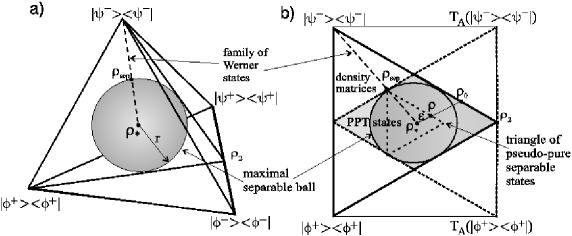
Figure 8: Maximal ball inscribed inside the $15$–D body ${\cal M}^{(4)}$ of mixed states is separable: a) $3$–D cross-section containing four Bell states, b) $2$–D cross–section defined by two Bell states and $\rho_{*}$ with the maximal separable triangle of pseudo-pure states.

For any $N\times N$ system the volume of the maximal separable ball, ${\bf B}^{\rm sep}_{N^{4}-1}$ may be compared with the Euclidean volume of ${\cal M}^{(N^{2})}$. The ratio

$$\frac{{\rm Vol}({\bf B}^{\rm sep}_{N^{4}-1})}{{\rm Vol}\bigl{(}{\cal M}^{(N^{2})}\bigr{)}}=\frac{\pi^{(N^{2}-1)/2}\,2^{(N^{2}-N^{4})/2}\,\Gamma(N^{4})}{\Gamma[(N^{4}+1)/2]\ N^{N^{4}}\,(N^{2}-1)^{(N^{4}-1)/2}\ \prod_{k=1}^{N^{2}}\Gamma(k)}$$ (62)

decreases fast with $N$, which suggests that for higher dimensional systems the separable states are not typical. The actual probability $p$ to find a separable mixed state is positive for any finite $N$ and depends on the measure used Zy99 ; Sl99 ; Sl04 . However, in the limit $N\to\infty$ the set of separable states is nowhere dense CH00 , so the probability $p$ computed with respect to an arbitrary non–singular measure tends to zero.

Another method of exploring the vicinity of the maximally mixed state consists in studying pseudo–pure states

$$\rho_{\epsilon}\equiv\frac{\mathbbm{1}}{N^{2}}(1-\epsilon)+\epsilon|\phi\rangle\langle\phi|\ ,$$ (63)

which are relevant for experiments with nuclear magnetic resonance (NMR) for $\epsilon\ll 1$. The set ${\cal M}_{\epsilon}$ is then defined as the convex hull of all $\epsilon$–pseudo pure states. It forms a smaller copy of the entire set of mixed states of the same shape and is centered at $\rho_{*}={\mathbbm{1}}/{N^{2}}$.

For instance, since the cross-section of the set ${\cal M}^{(4)}$ shown in Fig. 8b is a triangle, so is the set ${\cal M}_{\epsilon_{c}}$–a dashed triangle located inside the dark rhombus of separable states. The rhombus is obtained as a cross-section of the separable octahedron, which arises as a common part of the tetrahedron of density matrices spanned by four Bell states and its reflection representing their partial transposition HH96 ; Ar97 . An identical octahedron of super-positive maps will be formed by intersecting the tetrahedrons of CP and CcP one–qubit unital maps shown in Fig. 10.4. Properties of a separable octangula obtained for other 3-D cross-sections of ${\cal M}^{(4)}$ were analysed in Er02 . Several 2-D cross-sections plotted in JS01 ; VDM02 provide further insight into the geometry of the problem.

Making use of the radius (61) of the separable ball we obtain that the states ${\cal M}_{\epsilon}$ of a $N\times N$ bipartite system are separable for $\epsilon\leq\epsilon_{c}=1/(N^{2}-1)$. Bounds for $\epsilon_{c}$ in multipartite systems were obtained in BCJLPS99 ; DMK00 ; PR02 ; GB03 ; Sza04 ; GB04 . The size of the separable ball is large enough that to generate a genuinely entangled pseudo-pure state in an NMR experiment one would need to deal with at least $34$ qubits GB04 . Although experimentalist gained full control over $7-10$ qubits up till now, and work with separable states only, the NMR quantum computing does fine CFH97 ; CGKL98 ; LCNV02 .

Usually one considers states separable with respect to a given decomposition of the composed Hilbert space, ${\cal H}_{N^{2}}={\cal H}_{A}\otimes{\cal H}_{B}$. A state $\rho$ may be separable with respect to a given decomposition and entangled with respect to another one. Consider for instance, two decompositions of ${\cal H}_{6}$: ${\cal H}_{2}\otimes{\cal H}_{3}$ and ${\cal H}_{3}\otimes{\cal H}_{2}$ which describe different physical problems. There exist states separable with respect to the former decomposition and entangled with respect to the latter one. On the other hand one may ask, which states are separable with respect to all possible splittings of the composed system into subsystems $A$ and $B$. This is the case if $\rho^{\prime}=U\rho\,U^{\dagger}$ is separable for any global unitary $U$, and states possessing this property are called absolutely separable KZ01 .

All states belonging to the maximal ball inscribed into the set of mixed states for a bi-partite problem are not only separable but also absolutely separable. In the two–qubit case the set of absolutely separable states is larger than the maximal ball: As conjectured in IH00 and proved in VAM01 it contains any mixed state $\rho$ for which

$$C^{*}({\vec{x}})\ \equiv\ x_{1}-x_{3}-2\sqrt{x_{2}x_{4}}\leq 0\ ,$$ (64)

where ${\vec{x}}=\{x_{1}\geq x_{2}\geq x_{3}\geq x_{4}\}$ denotes the ordered spectrum of $\rho$. The problem, whether there exist absolutely separable states outside the maximal ball was solved for $2\times 3$ case Hi05 , but it remains open in higher dimensions. Numerical investigations suggest that in such a case the set ${\cal M}_{S}$ of separable states, located in central parts of ${\cal M}$, is covered by a shell of bound entangled states. However this shell is not perfect, in the sense that the set of NPPT entangled states (occupying certain ’corners’ of ${\cal M}$) has a common border with the set of separable states.

Some insight into the geometry of the problem may be gained by studying the manifold $\Sigma$ of mixed products states. To verify whether a given state $\rho$ belongs to $\Sigma$ one computes the partial traces and checks if $\rho_{A}\otimes\rho_{B}$ is equal to $\rho$. This is the case e.g. for the maximally mixed state, $\rho_{*}\in\Sigma$. All states tangent to $\Sigma$ at $\rho_{*}$ are separable, while the normal subspace contains the maximally entangled states. Furthermore, for any bi-partite systems the maximally mixed state $\rho_{*}$ is the product state closest to any maximally entangled state (with respect to the HS distance) LSG02 .

Let us return to characterisation of the boundary of the set of separable states for a bi-partite system. For any entangled state $\sigma_{\rm ent}$ one may define the separable state $\sigma_{\rm sep}\in\partial{\cal M}_{S}$, which is closest to $\sigma_{\rm ent}$ with respect to a given metric. In general it is not easy to find the closest separable state, even in the two qubit case, for which the $14$-dim boundary of the set ${\cal M}_{S}^{(4)}$ may be characterised explicitly,

$$(\rho\in\partial{\cal M}_{S}^{(4)})\ \Rightarrow\ {\rm det}\rho=0{\quad\rm or\quad}{\rm det}\rho^{T_{A}}=0\ .$$ (65)

Alternatively, for any entangled state one defines the best separable approximation also called Lewenstein–Sanpera decomposition LS98 ,

$$\rho_{\rm ent}\ =\ \Lambda\rho_{\rm sep}+(1-\Lambda)\rho_{b},$$ (66)

where the separable state $\rho_{sep}$ and the state $\rho_{b}$ are chosen in such a way that the positive weight $\Lambda\in[0,1]$ is maximal. Uniqueness of such a decomposition was proved in LS98 for two qubits, and in KL01 for any bi–partite system. In the two–qubit problem the state $\rho_{b}$ is pure, and is maximally entangled for any full rank state $\rho$ KL01 . An explicit form of the decomposition (66) was found in WK01 for a generic two–qubit state and in AJ04 for some particular cases in higher dimensions. Note the key difference in both approaches: looking for the separable state closest to $\rho$ we probe the boundary $\partial{\cal M}^{(N)}_{S}$ of the set of separable states only, while looking for its best separable approximation we must also take into account the boundary of the entire set of density matrices – compare Figs. 9a. and 10a.

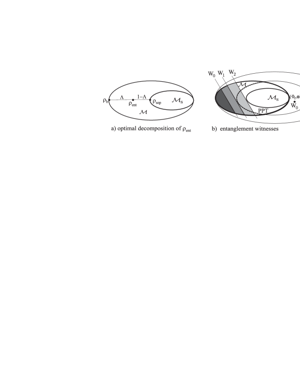
Figure 9: a) Best separable approximation of entangled state $\rho$; b) a witness $W_{0}$ detects entanglement in a subset of entanglement states; $W_{1}$ – optimal decomposable witness; $W_{2}$ – optimal non–decomposable witness.

The structure of the set of separable states may also be analyzed with use of the entanglement witnesses PR03 , already defined in the previous section. Any witness $W$, being a non-positive operator, may be represented as a point located far outside the set ${\cal M}$ of density matrices, in its image with respect to an extended positive map, $(\Phi_{\cal P}\otimes{\mathbbm{1}})$, or as a line perpendicular to the axis $OW$ which crosses ${\cal M}$. The states outside this line satisfy Tr$\rho W<0$, hence their entanglement is detected by $W$. A witness $W_{1}$ is called finer than $W_{0}$ if every entangled state detected by $W_{0}$ is also detected by $W_{1}$. A witness $W_{2}$ is called optimal if the corresponding map belongs to the boundary of the set of positive operators, so the line representing $W_{2}$ touches the boundary of the set ${\cal M}_{S}$ of separable states. A witness related to a generic non CP map $\Phi_{\cal P}\in{\cal P}$ may be optimized by sending it toward the boundary of ${\cal P}$ LKCHC00 . If a positive map $\Phi_{\cal D}$ is decomposable, the corresponding witness, $W=D_{\Phi_{\cal D}}/N$ is called decomposable. Any decomposable witness cannot detect PPT bound entangled states - see Fig. 9b.

One might argue that in general a witness $W=D_{\Phi}/N$ is theoretically less useful than the corresponding map $\Phi$, since the criterion Tr$\rho W<0$ is not as powerful as $N(W^{R}\rho^{R})^{R}=(\Phi\otimes{\mathbbm{1}})\rho\geq 0$. However, a non–CP map $\Phi$ cannot be realised in nature, while an observable $W$ may be measured. Suitable witness operators were actually used to detect quantum entanglement experimentally in bi–partite BMNMAM03 ; GHDELMS03 and multi–partite systems BEKWGHBLS04 . Furthermore, the Bell inequalities may be viewed as a kind of separability criterion, related to a particular entanglement witness Te00b ; HHH00b ; HGBL05 , so evidence of their violation for certain states ADR82 might be regarded as an experimental detection of quantum entanglement.

VII Entanglement measures

We have already learned that the degree of entanglement of any pure state of a $N\times K$ system may be characterised by the entanglement entropy (25) or any other Schur concave function $f$ of the Schmidt vector $\vec{\lambda}$. The problem of quantifying entanglement for mixed states becomes complicated VPRK97 ; DHR02 ; HoM01 .

Let us first discuss the properties that any potential measure $E(\rho)$ should satisfy. Even in this respect experts seem not to share exactly the same opinions BVSW96 ; PR97 ; VP98 ; Vi00 ; HHH00 .

There are three basic axioms,

(E1) Discriminance. $E(\rho)=0$ if and only if $\rho$ is separable,

(E2) Monotonicity (29) under probabilistic LOCC,

(E3) Convexity,  $E\bigl{(}a\rho+(1-a)\sigma\bigr{)}\leq aE(\rho)+(1-a)E(\sigma)$, with $a\in[0,1]$.

Then there are certain additional requirements,

(E4) Asymptotic continuity (We follow HoM01 here; slightly different fomulations of this property are used in HHH00 ; DHR02 ), Let $\rho_{m}$ and $\sigma_{m}$ denote sequences of states acting on $m$ copies of the composite Hilbert space, $({\cal H}_{N}\otimes{\cal H}_{K})^{\otimes m}$.

$${\rm If\quad}\lim_{m\to\infty}||\rho_{m}-\sigma_{m}||_{1}=0{\quad\rm then\quad}\lim_{m\to\infty}\frac{E(\rho_{m})-E(\sigma_{m})}{m\ln NK}=0\ ,$$ (67)

(E5) Additivity. $E(\rho\otimes\sigma)\ =\ E(\rho)+E(\sigma)$ for any $\rho,\sigma\in{\cal M}_{NK}$,

(E6) Normalisation. $E(|\psi^{-}\rangle\langle\psi^{-}|)=1$,

(E7) Computability.  There exists an efficient method to compute $E$ for any $\rho$.

There are also alternative forms of properties (E1-E5),

(E1a) Weak discriminance.  If $\rho$ is separable then $E(\rho)=0$,

(E2a) Monotonicity under deterministic LOCC,  $E(\rho)\geq E[\Phi_{\rm LOCC}(\rho)]$,

(E3a) Pure states convexity.   $E(\rho)\leq\sum_{i}p_{i}E(\phi_{i})$ where $\rho=\sum_{i}p_{i}|\phi_{i}\rangle\langle\phi_{i}|$,

(E4a) Continuity.  If $||\rho-\sigma||_{\rm 1}\to 0$ then $|E(\rho)-E(\sigma)|\to 0$.

(E5a) Extensivity.  $E(\rho^{\otimes n})=nE(\rho)$.

(E5b) Subadditivity.  $E(\rho\otimes\sigma)\ \leq\ E(\rho)+E(\sigma)$.

(E5c) Superadditivity.  $E(\rho\otimes\sigma)\ \geq\ E(\rho)+E(\sigma)$.

The above list of postulates deserves a few comments. The rather natural ’if and only if’ condition in (E1) is very strong: it cannot be satisfied by any measure quantifying the distillable entanglement, due to the existence of bound entangled states. Hence one often requires the weaker property (E1a) instead.

Monotonicity (E2) under probabilistic transformations is stronger than monotonicity (E2a) under deterministic LOCC. Since local unitary operations are reversible, the latter property implies

(E2b) Invariance with respect to local unitary operations,

$$E(\rho)=E(U_{A}\otimes U_{B}\,\rho\,U_{A}^{\dagger}\otimes U_{B}^{\dagger})\ .$$ (68)

Convexity property (E3) guarantees that one cannot increase entanglement by mixing. Following Vidal Vi00 , we will call any quantity satisfying (E2) and (E3) an entanglement monotone (Some authors require also continuity (E4a)). These fundamental postulates reflect the key idea that quantum entanglement cannot be created locally. Or in more economical terms: it is not possible to get any entanglement for free – one needs to invest resources for certain global operations.

The postulate that any two neighbouring states should be characterised by similar entanglement is made precise in (E4). Let us recall here the Fannes continuity lemma (13.36), which estimates the difference between von Neumann entropies of two neighbouring mixed states. Similar bounds may also be obtained for any other Rényi entropy with $q>0$, but then the bounds for $S_{q}$ are weaker then for $S_{1}$. Although $S_{q}$ are continuous for $q>0$, in the asymptotic limit $n\to\infty$ only $S_{1}$ remains a continuous function of the state $\rho^{\otimes n}$. In the same way the asymptotic continuity distinguishes the entanglement entropy based on $S_{1}$ from other entropy measures related to the generalised entropies $S_{q}$ Vi00 ; DHR02 .

Additivity (E5) is a most welcome property of an optimal entanglement measure. For certain measures one can show sub- or super–additivity; additivity requires both of them. Unfortunately this is extremely difficult to prove for two arbitrary density matrices, so some authors suggest to require extensivity (E5a). Even this property is not easy to demonstrate. However, for any measure $E$ one may consider the quantity

$$E_{R}(\rho)\ \equiv\ \lim_{n\to\infty}\frac{1}{n}E(\rho^{\otimes n})\ .$$ (69)

If such a limit exists, then the regularised measure $E_{R}$ defined in this way satisfies (E5a) by construction. The normalisation property (E6), useful to compare different quantities, can be achieved by a trivial rescaling.

The complete wish list (E1-E7) is very demanding, so it is not surprising that instead of one ideal measure of entanglement fulfilling all required properties, the literature contains a plethora of measures VP98 ; HoM01 ; Br02 , each of them satisfying some axioms only… The pragmatic wish (E7) is an especially tough one—since we have learned that even the problem of deciding the separability is a ’hard one’ Gu03 ; Gu04 , the quantifying of entanglement cannot be easier. Instead of waiting for the discovery of a single, universal measure of entanglement, we have thus no choice but to review some approaches to the problem. In the spirit of this book we commence with

I. Geometric measures

The distance from an analysed state $\rho$ to the set ${\cal M}_{S}$ of separable states satisfies (E1) by construction – see Fig. 10a. However, it is not simple to find the separable state $\sigma$ closest to $\rho$ with respect to a certain metric, necessary to define $D_{x}(\rho)\equiv D_{x}(\rho,\sigma)$. There are several distances to choose from, for instance

G1. Bures distance VP98 $D_{\rm B}(\rho)\equiv\min_{\sigma\in{\cal M}_{S}}D_{\rm B}(\rho,\sigma)$,

G2. Trace distance EAP03 $D_{\rm Tr}(\rho)\equiv\min_{\sigma\in{\cal M}_{S}}D_{\rm Tr}(\rho,\sigma)$,

G3. Hilbert-Schmidt distance WT99 $D_{\rm HS}(\rho)\equiv\min_{\sigma\in{\cal M}_{S}}D_{\rm HS}(\rho,\sigma)$.

The Bures and the trace metrics are monotone (see section 13.2 and 14.1), which directly implies (E2a), while $D_{\rm B}$ fulfils also the stronger property (E2) VP98 . Since the HS metric is not monotone Oz01 it is not at all clear, whether the minimal Hilbert–Schmidt distance is an entanglement monotone VDM02 . Since the diameter of the set of mixed states with respect to the above distances is finite, all distance measures cannot satisfy even the partial additivity (E3a).

Although quantum relative entropy is not exactly a distance, but rather a contrast function, it may also be used to characterise entanglement.

G4. Relative entropy of entanglement VPRK97 $D_{R}(\rho)\equiv\min_{\sigma\in{\cal M}_{S}}S(\rho||\sigma)$.

In view of the discussion in chapter 13 this measure has an appealing interpretation as distinguishability of $\rho$ from the closest separable state. For pure states it coincides with the entanglement entropy, $D_{R}(|\phi\rangle)=E_{1}(|\phi\rangle)$ VP98 . Analytical formulae for $D_{R}$ are known in certain cases only VPRK97 ; VW01 ; Is03 , but it may be efficiently computed numerically RH03 . This measure of entanglement is convex (due to double convexity of relative entropy) and continuous DH99 , but not additive VW01 . It is thus useful to study the regularised quantity, $\lim_{n\to\infty}D_{R}(\rho^{\otimes n})/n$. This limit exists due to subadditivity of relative entropy and has been computed in some cases AEJPVM01 ; AMVW02 .

G5. Reversed relative entropy of entanglement $D_{RR}(\rho)\equiv\min_{\sigma\in{\cal M}_{S}}S(\sigma||\rho)$.

This quantity with exchanged arguments is not so interesting per se, but its modification $D_{RR}^{\prime}$ – the minimal entropy with respect to the set ${\cal M}_{\rho}$ of separable states $\rho^{\prime}$ locally identical to $\rho$, $\{\rho^{\prime}\in{\cal M}_{\rho}:\rho^{\prime}_{A}=\rho_{A}$ and $\rho^{\prime}_{B}=\rho_{B}\}$, provides a distinctive example of an entanglement measure, which satisfies the additivity condition (E3) EAP03 . (A similar measure based on modified relative entropy was introduced by Partovi Pa04 .)

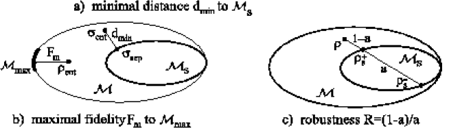
Figure 10: a) Minimal distance $D_{x}$ to the closest separable state. b) Maximal fidelity to a maximally entangled state. c) Robustness, i.e. the minimal ratio of the distance to set ${\cal M}_{S}$ by its width.

G6. Robustness VT99 . $R(\rho)$ measures the endurance of entanglement by quantifying the minimal amount of mixing with separable states needed to wipe out the entanglement,

$$R(\rho)\equiv\min_{\rho_{s}^{-}\in{\cal M}_{S}}\Bigl{(}\min_{s\geq 0}\ s:\rho_{s}^{+}=\frac{1}{1+s}(\rho+s\rho_{s}^{-})\in{\cal M}_{S}\Bigr{)}\ .$$ (70)

As shown if Fig. 10c the robustness $R$ may be interpreted as a minimal ratio of the HS distance $1-a=s/(1+s)$ of $\rho$ to the set ${\cal M}_{S}$ of separable states to the width $a=1/(1+s)$ of this set. This construction does not depend on the boundary of the entire set ${\cal M}$, in contrast with the best separable approximation. (In the two-qubit case the entangled state used for BSA (66) is pure, $\rho_{b}=|\phi_{b}\rangle\langle\phi_{b}|$, the weight $\Lambda$ is a monotone EB01 , so the quantity $(1-\Lambda)E_{1}(\phi_{b})$ works as a measure of entanglement LS98 ; WK01 ). Robustness is known to be convex and monotone, but is not additive VT99 . Robustness for two–qubit states diagonal in the Bell basis was found in AJ03 , while a generalisation of this quantity was proposed in St03 .

G7. Maximal fidelity $F_{m}$ with respect to the set ${\cal M}_{\rm max}$ of maximally entangled states BVSW96 , $F_{m}(\rho)\equiv\max_{\phi\in{\cal M}_{\rm max}}F(\rho,|\phi\rangle\langle\phi|)$.

Strictly speaking the maximal fidelity cannot be considered as a measure of entanglement, since it does not satisfy even weak discriminance (E1a). However, it provides a convenient way to characterize, to what extent $\rho$ may approximate a maximally entangled state required for various tasks of quantum information processing, so in the two-qubit case it is called the maximal singlet fraction. Invoking (9.31) we see that $F_{m}$ is a function of the minimal Bures distance from $\rho$ to the set ${\cal M}_{\rm max}$. An explicit formula for the maximal fidelity for a two-qubit state was derived in BHHH00 , while relations to other entanglement measures were analysed in VV02b .

II. Extensions of pure–state measures

Another class of mixed–states entanglement measures can be derived from quantities characterizing entanglement of pure states. There exist at least two different ways of proceeding. The convex roof construction Uh98 ; Uh03 defines $E(\rho)$ as the minimal average quantity $\langle E(\phi)\rangle$ taken on pure states forming $\rho$. The most important measure is induced by the entanglement entropy (25).

P1. Entanglement of Formation (EoF) BVSW96

$$E_{F}(\rho)\ \equiv\ \min_{{\cal E}_{\rho}}\sum_{i=1}^{M}p_{i}E_{1}(|\phi_{i}\rangle)\ ,$$ (71)

where the minimisation

is performed over an ensemble of all possible decompositions

$${\cal E}_{\rho}=\{p_{i},|\phi_{i}\rangle\}_{i=1}^{M}\ :\ \rho=\sum_{i=1}^{M}p_{i}|\phi_{i}\rangle\langle\phi_{i}|{\rm\quad with\quad}p_{i}>0,\quad\sum_{i=1}^{M}p_{i}=1\ .$$ (72)

(A dual quantity defined by maximisation over ${\cal E}_{\rho}$ is called entanglement of assistance DFMSTU99 , and both of them are related to relative entropy of entanglement of an extended system HV00 .)

The ensemble ${\cal E}$ for which the minimum (71) is realised is called optimal. Several optimal ensembles might exist, and the minimal ensemble length $M$ is called the cardinality of the state $\rho$. If the state is separable then $E_{F}(\rho)=0$, and the cardinality coincides with the minimal length of the decomposition (37). Due to Carathéodory’s theorem the cardinality of $\rho\in{\cal M}^{NK}$ does not exceed the squared rank of the state, $r^{2}\leq N^{2}K^{2}$ Uh98 . In the two-qubit case it is sufficient to take $M=4$ Wo98 , and this length is necessary for some states of rank $r=3$ AVM01 . In higher dimensions there exists states for which $M>NK\geq r$ DTT00 .

Entanglement of formation enjoys several appealing properties: it may be interpreted as the minimal pure–states entanglement required to build up the mixed state. It satisfies by construction the discriminance property (E1) and is convex and monotone BVSW96 . EoF is known to be continuous Ni00b , and for pure states it is by construction equal to the entanglement entropy $E_{1}(|\phi\rangle)$. To be consistent with normalisation (E6) one often uses a rescaled quantity, $E_{F}^{\prime}\equiv E_{F}/\ln 2$.

Two other properties are still to be desired, if EoF is to be an ideal entanglement measure: we do not know, whether EoF is additive and EoF is not easy to evaluate. Additivity of EoF has been demonstrated in special cases only, if one of the states is a product state BN01 , is separable VW01 or if it is supported on a specific subspace VDC02 . At least we can be sure that EoF satisfies subadditivity (E5b), since the tensor product of the optimal decompositions of $\rho$ and $\sigma$ provides an upper bound for $E(\rho\otimes\sigma)$.

Explicit analytical formulae were derived for the two-qubit system Wo98 , and a certain class of symmetric states in higher dimensions TVo00 ; VW01 , while for the $2\times K$ systems at least lower bounds are known CLLH02 ; LBZW03 ; Ge03 . Numerically EoF may by estimated by minimisation over the space of unitary matrices $U(M)$. A search for the optimal ensemble can be based on simulated annealing Zy99 , on a faster conjugate–gradient method AVM01 , or on minimising the conditional mutual information Tu01 .

P2. Generalised Entanglement of Formation (GEoF)

$$E_{q}(\rho)\ \equiv\ \min_{{\cal E}_{\rho}}\sum_{i=1}^{M}p_{i}\,E_{q}(|\phi_{i}\rangle)\ ,$$ (73)

where $E_{q}(|\phi\rangle)=S_{q}[{\rm Tr}_{B}(|\phi\rangle\langle\phi|)]$ stands for the Rényi entropy of entanglement. Note that an optimal ensemble for a certain value of $q$ needs not to provide the minimum for $q^{\prime}\neq q$. GEoF is asymptotically continuous only in the limit $q\to 1$ for which it coincides with EoF. In the very same way, the convex roof construction can be applied to extend any pure states entanglement measure for mixed states. In fact, several measures introduced so far are related to GEoF. For instance, the convex roof extended negativity LCOK03 and concurrence of formation Woo01 ; RC03 ; MKB04 are related to $E_{1/2}$ and $E_{2}$, respectively.

There is another way to make use of pure state entanglement measures. In analogy to the fidelity between two mixed states, equal to the maximal overlap between their purifications, one may also purify $\rho$ by a pure state $|\psi\rangle\in({\cal H}_{N}\otimes{\cal H}_{K})^{\otimes 2}$. Based on the entropy of entanglement (25) one defines

P3. Entanglement of purification THLV02 ; BB02

$$E_{P}(\rho)\ \ \ \equiv\ \ \ \ \min_{|\phi\rangle:\ \rho={\rm Tr}_{KN}(|\phi\rangle\langle\phi|)}E_{1}(|\phi\rangle)\ ,$$ (74)

but any other measure of pure states entanglement might be used instead.

The entanglement of purification is continuous and monotone under strictly local operations (not under LOCC). It is not convex, but more importantly, it does not satisfy even the weak discriminance (E1a). In fact $E_{P}$ measures correlations between both subsystems, and is positive for any non-product, separable mixed state BB02 . Hence entanglement of purification is not an entanglement measure, but it happens to be helpful to estimate a variant of the entanglement cost THLV02 . To obtain a reasonable measure one needs to allow for an arbitrary extension of the system size, as assumed by defining

P4. Squashed entanglement CW04

$$E_{S}(\rho^{AB})\ \ \ \equiv\ \ \ \ \inf_{\rho^{ABE}}{\frac{1}{2}\bigl{[}S(\rho^{AE})+S(\rho^{BE})-S(\rho^{E}})-S(\rho^{ABE})\bigr{]}\ ,$$ (75)

where the infimum is taken over all extensions $\rho^{ABE}$ of an unbounded size such that ${\rm Tr}_{E}(\rho^{ABE})=\rho^{AB}$. Here $\rho^{AE}$ stands for ${\rm Tr}_{B}(\rho^{ABE})$ while $\rho^{E}={\rm Tr}_{AB}(\rho^{ABE})$. Minimized quantity is proportional to quantum conditional mutual information of $\rho^{ABE}$ Tu01 and its name refers to ’squashing out’ the classical correlations.

Squashed entanglement is convex, monotone and vanishes for every separable state CW04 . If $\rho^{AB}$ is pure then $\rho^{ABE}=\rho^{E}\otimes\rho^{AB}$, hence $E_{S}=[S(\rho^{A})+S(\rho^{B})]/2=S(\rho^{A})$ and the squashed entanglement reduces to the entropy of entanglement $E_{1}$. It is charactarised by asymptotic continuity AF04 , and additivity (E5), which is a consequence of the strong subadditivity of the von Neumann entropy CW04 . Thus $E_{S}$ would be a perfect measure of entanglement, if we only knew how to compute it…

III. Operational measures

Entanglement may also be quantified in an abstract manner by considering the minimal resources required to generate a given state or the maximal entanglement yield. These measures are defined implicitly, since one deals with an infinite set of copies of the state analysed and assumes an optimisation over all possible LOCC protocols.

O1. Entanglement cost BVSW96 ; Ra99 $E_{C}(\rho)=\lim_{n\to\infty}\frac{m}{n}$ where $m$ is the number of singlets $|\psi^{-}\rangle$ needed to produce locally $n$ copies of the analysed state $\rho$.

Entanglement cost has been calculated for instance for states supported on a subspace such that tracing out one of the parties forms an entanglement breaking channel (super separable map) VDC02 . Moreover, entanglement cost was shown HHT01 to be equal to the regularised entanglement of formation, $E_{C}(\rho)=\lim_{n\to\infty}E_{F}(\rho^{\otimes n})/n$. Thus, if we knew that EoF is additive, the notions of entanglement cost and entanglement of formation would coincide…

O2. Distillable entanglement BVSW96 ; Ra99 . $E_{D}(\rho)=\lim_{n\to\infty}\frac{m}{n}$ where $m$ is the maximal number of singlets $|\psi^{-}\rangle$ obtained out of $n$ copies of the state $\rho$ by an optimal LOCC conversion protocol.

Distillable entanglement is a measure of a fundamental importance, since it tells us how much entanglement one may extract out of the state analysed and use e.g. for the cryptographic purposes. It is rather difficult to compute, but there exist analytical bounds due to Rains Ra99b ; Ra01 , and an explicit optimisation formula was found DW05 . $E_{D}$ is not likely to be convex SST01 , although it satisfies the weaker condition (E3a) DHR02 .

IV. Algebraic measures

If a partial transpose of a state $\rho$ is not positive then $\rho$ is entangled due to the PPT criterion B1. The partial transpose preserves the trace, so if $\rho^{T_{A}}\geq 0$ then $||\rho^{T_{A}}||_{\rm Tr}={\rm Tr}\rho^{T_{A}}=1$. Hence we can use the trace norm to characterize the degree, to which the positivity of $\rho^{T_{A}}$ is violated.

N1. Negativity ZHSL98 ; EP99 ,  ${\cal N}_{T}(\rho)\equiv||\rho^{T_{A}}||_{\rm Tr}-1$.

Negativity is easy to compute, convex (partial transpose is linear and the trace norm is convex) and monotone Ei01 ; ViWe02 . It is not additive, but this drawback may be cured by defining the log–negativity $\ln||\rho^{T_{A}}||_{\rm Tr}$. It was used by Rains Ra01 to obtain bounds on distillable entanglement. However, the major deficiency of the negativity is its failure to satisfy (E1) – by construction ${\cal N}_{T}(\rho)$ cannot detect PPT bound entangled states. In the two–qubit case the spectrum of $\rho^{T_{A}}$ contains at most a single negative eigenvalue STV98 , so ${\cal N}^{\prime}_{T}\equiv{\rm max}\{0,-2\lambda_{\rm min}\}={\cal N}_{T}$. This observation explains the name on the one hand, and on the other provides a geometric interpretation: ${\cal N}_{T}^{\prime}(\rho)$ measures the minimal relative weight of the maximally mixed state $\rho_{*}$ which needs to be mixed with $\rho$ to produce a separable mixture VDM02 . In higher dimensions several eigenvalues of the partially transposed state may be negative, so in general ${\cal N}_{T}\neq{\cal N}^{\prime}_{T}$, and the latter quantity is proportional to complete co–positivity (11.13) of a map $\Phi$ associated with the state $\rho$.

Negativity is not the only application of the trace norm ViWe02 . Building on the positive maps criterion A1 for separability one might analyse analogous quantities for any (not completely) positive map, ${\cal N}_{\Phi}(\rho)\equiv||(\Phi\otimes{\mathbbm{1}})\rho||_{\rm Tr}-1$. Furthermore, one may consider another quantity related to the reshuffling criterion B6.

N2. Reshuffling negativity CW02 ; Rud03 . ${\cal N}_{R}(\rho)\equiv||\rho^{R}||_{\rm Tr}-1$.

This quantity is convex due to linearity of reshuffling and non-increasing under local measurements, but may increase under partial trace Rud03 . For certain bound entangled states ${\cal N}_{R}$ is positive; unfortunately not for all of them… A similar quantity with the minimal cross-norm $||\cdot||_{\gamma}$ was studied by Rudolph Rud01 , who showed that ${\cal N}_{\gamma}(\rho)=||\rho||_{\gamma}-1$ is convex and monotone under local operations. However, $||\rho^{R}||_{\rm Tr}$ is easily computable from the definition (10.33), in contrast to $||\rho||_{\gamma}$.

Table 2: Properties of entanglement measures: discriminance E1, monotonicity E2, convexity E3, asymptotic continuity E4, additivity E5, extensivity E5a, computability E7: explicit closed formula C, optimisation over a finite space F or an infinite space I; Rényi parameter $q$ for pure states.

computab q Entanglement measure	E1	E2	E3	E4	E5	E5a	E7	$q$
G1 Bures distance $D_{B}$	Y	Y	Y	N	N	N	F	$2$
G2 Trace distance $D_{\rm Tr}$	Y	Y	Y	N	N	N	F
G3 HS distance $D_{\rm HS}$	Y	?	?	N	N	N	F
G4 Relative entropy $D_{R}$	Y	Y	Y	Y	N	?	F	$1$
G5’ reversed RE, $D_{RR}^{\prime}$	?	Y	Y	Y	Y	Y	F	$1$
G6 Robustness $R$	Y	Y	Y	N	N	N	F	$1/2$
P1 Entangl. of formation $E_{F}$	Y	Y	Y	Y	?	?	C/F	$1$
P2 Generalised EoF, $E_{q}$	Y	Y	?	N	?	?	F	$q$
P4 Squashed entangl. $E_{S}$	?	Y	Y	Y	Y	Y	I	$1$
O1 Entan. cost $E_{C}$	Y	Y	Y	Y	?	Y	I	$1$
O2 Distillable entangl. $E_{D}$	N	Y	N(?)	Y	?	Y	I	$1$
N1 Negativity ${\cal N}_{T}$	N	Y	Y	N	N	N	C	$1/2$
N2 Reshuffling negativity ${\cal N}_{R}$	N	N	Y	N	N	N	C	$1/2$

There exists also attempts to quantify entanglement by the dynamical properties of a state and the speed of decoherence BJO01 , or the secure key distillation rate HHHO05 ; DW05 and several others… For multipartite systems the problem gets even more demanding CKW00 ; EB01 ; WG03 ; Pa04 .

We end this short tour through the vast garden of entanglement measures, by studying how they behave for pure states. Entanglement of formation and purification coincide by construction with the entanglement entropy $E_{1}$. So is the case for both operational measures, since conversion of $n$ copies of an analyzed pure state into $m$ maximally entangled states is reversible. The negativities are easy to compute. For any pure state $|\psi\rangle\in{\cal H}_{N}\otimes{\cal H}_{N}$ written in the Schmidt form, the non-zero entries of the density matrix $\rho_{\psi}$ of size $N^{2}$ are equal to $\sqrt{\lambda_{i}\lambda_{j}}$, $i,j=1,\dots,N$. The reshuffled matrix $\rho_{\psi}^{R}$ becomes diagonal, while partially transposed matrix $\rho_{\psi}^{T_{2}}$ has a block structure: it consists of $N$ Schmidt components $\lambda_{i}$ at the diagonal which sum to unity and $N(N-1)/2$ off-diagonal blocks of size $2$, one for each pair of different indices $(i,j)$. Eigenvalues of each block are $\pm\sqrt{\lambda_{i}\lambda_{j}}$, so both traces norms are equal to the sum of all entries. Hence both negativities coincide for pure states,

$${\cal N}_{T}(\rho_{\psi})={\cal N}_{R}(\rho_{\psi})=\sum_{i,j=1}^{N}\!\!\sqrt{\lambda_{i}\lambda_{j}}-1=\bigr{(}\sum_{i}^{N}\!\!\sqrt{\lambda_{i}}\bigl{)}^{2}-1=e^{E_{1/2}}-1\ ,$$ (76)

and vary from $0$ for separable states to $N-1$ for maximally entangled states. Also maximal fidelity and robustness for pure states become related, $F=\exp(E_{1/2})/N$ and $R={\cal N}_{T}=\exp(E_{1/2})-1$ VT99 . On the other hand, the minimal Bures distance to the closest separable (mixed) state VP98 becomes a function of the Rényi entropy of order two,

$$D_{\rm B}(\rho_{\phi})=\bigl{(}2-2\sum_{i=1}\lambda_{i}^{2}\bigr{)}^{1/2}=\sqrt{2-2e^{-E_{2}/2}}\ ,$$ (77)

and is equal to concurrence (26), while the Bures distance to the closest separable pure state $D_{\rm B}^{\rm pure}(|\phi\rangle)=[2(1-\sqrt{1-\lambda_{max}})]^{1/2}$ is a function of $E_{\infty}=-\ln\lambda_{\rm max}$. The Rényi parameters $q$ characterising behaviour of the discussed measures of entanglement for pure states are collected in Table 2.

Knowing that a given state $\rho$ can be locally transformed into $\rho^{\prime}$ implies that $E(\rho)\geq E(\rho^{\prime})$ for any measure $E$, but the converse is not true. Two Rényi entropies of entanglement of different (positive) orders generate different order in the space of pure states. By continuity this is also the case for mixed states, and the relation

$$E_{A}(\rho_{1})\>\leq\>E_{A}(\rho_{2})\ \ \Leftrightarrow\ \ E_{B}(\rho_{1})\>\leq\>E_{B}(\rho_{2})$$ (78)

does not hold. For a certain pair of mixed states it is thus likely that one state is more entangled with respect to a given measure, while the other one, with respect to another measure of entanglement EP99 . If two measures $E_{A}$ and $E_{B}$ coincide for pure states they are identical or they do not generate the same order in the set of mixed states VP00 . Hence entanglement of formation and distillable entanglement do not induce the same order. On the other hand, several entanglement measures are correlated and knowing $E_{A}$ one may try to find lower and upper bounds for $E_{B}$.

The set of entanglement measures shrinks, if one imposes even some of the desired properties (E1)-(E7). The asymptotic continuity (E4) is particularly restrictive. For instance, among generalized Rényi entropies it is satisfied only by the entropy of entanglement $E_{1}$ Vi00 . If a measure $E$ satisfies additionally monotonicity (E2a) under deterministic LOCC and extensivity (E5a), it is bounded by the distillable entanglement and entanglement cost HHH00 ; HoM01 ,

$$E_{D}(\rho)\ \leq\ E(\rho)\ \leq\ E_{C}(\rho)\ .$$ (79)

Interestingly, the two first measures introduced in the pioneering paper by Bennett et al. BVSW96 occurred to be the extreme entanglement measures. For pure states both of them coincide, and we arrive at a kind of uniqueness theorem: Any monotone, extensive and asymptotically continuous entanglement measure coincides for pure states with the entropy of formation $E_{F}$ PR97 ; Vi00 ; DHR02 . This conclusion concerning pure states entanglement of bipartite systems may also be reached by an abstract, thermodynamic approach VK02 .

Let us try to recapitulate the similarities and differences between four classes of entanglement measures. For a geometric measure or an extension of a pure states measure it is not simple to check, which of the desired properties are satisfied. Furthermore, to evaluate it for a typical mixed state one needs to perform a cumbersome optimisation scheme. One should not expect the remarkable analytical result of Wootters Wo98 for entanglement of formation in the $2\times 2$ system, to be extended for the general $N\times N$ problem, since even stating the separability is known to be an algorithmically complex task Gu03 .

Operational measures are nice, especially from the point of view of information science, and extensivity and monotonicity are direct consequence of their definitions. However, they are extremely hard to compute. In contrast, algebraic measures are easy to calculate, but they fail to detect entanglement for all non–separable states. Summarising, several different measures of entanglement are thus likely to be still used in future…

VIII Two qubit mixed states

Before discussing the entanglement of two–qubit mixed states let us recapitulate, in what sense the case $N=2$ differs from $N\geq 3$.

A)  algebraic properties

i)   $SU(N)\times SU(N)$ is homomorphic to $SO(N^{2})$ for $N=2$ only,

ii)  $SU(N)\cong SO(N^{2}-1)$ for $N=2$ only,

iii) All positive maps $\Phi:{\cal M}^{(N)}\to{\cal M}^{(N)}$ are decomposable for $N=2$ only,

B)  $N$–level mono-partite systems

iv) Boundary $\partial{\cal M}^{(2)}$ consists of pure states only,

v)  For any state $\rho_{\vec{\tau}}$ $\in{\cal M}^{(N)}$ also its antipode $\rho_{-{\vec{\tau}}}=2\rho_{*}-\rho_{\vec{\tau}}$ forms a state and there exists a universal NOT operation for $N=2$ only.

vi)  ${\cal M}^{(N)}\subset{\mathbb{R}}^{N^{2}-1}$ forms a ball for $N=2$ only,

C)  $N\times N$ composite systems

vii) For any pure state $|\psi\rangle\in{\cal H}_{N}\otimes{\cal H}_{N}$ there exist $N-1$ independent Schmidt coefficients $\lambda_{i}$. For $N=2$ there exists only one independent coefficient $\lambda_{1}$, hence all entanglement measures are equivalent.

viii) The maximally entangled states form the manifold $SU(N)/{\mathbb{Z}}_{N}$, which is equivalent to the real projective space ${\mathbb{R}}{\bf P}^{N^{2}-1}$ only for $N=2$.

ix)   All PPT states of a $N\times N$ system are separable for $N=2$ only.

x)    For any two–qubit mixed state its optimal decomposition consists of pure states of equal concurrence. Thus entanglement of formation becomes a function of concurrence of formation for $2\times 2$ systems.

These features demonstrate why entanglement of two-qubit systems is special VW00 . Several of these issues are closely related. We have already learned that decomposability iii) is a consequence of ii) and implies the separability ix). We shall see now, how a group-theoretic fact i) allows one to to derive a closed formula for EoF of a two qubit system. We are going to follow the seminal paper of Wootters Wo98 , who built up on his earlier work with Bennett et al. BVSW96 and the paper with Hill HW97 .

Consider first a two–qubit pure state $|\psi\rangle$. Due to its normalisation the Schmidt components—eigenvalues of the matrix $\Gamma\Gamma^{\dagger}$ —satisfy $\mu_{1}+\mu_{2}=1$. The tangle of $|\psi\rangle$, defined in (26), reads

$$\tau=C^{2}=2(1-\mu_{1}^{2}-\mu_{2}^{2})=4\mu_{1}(1-\mu_{1})=4\mu_{1}\mu_{2}\ ,$$ (80)

and implies that concurrence is proportional to the determinant of (8),

$$C=2\ |\sqrt{\mu_{1}\mu_{2}}|=2\ |{\rm det}\Gamma|\ .$$ (81)

Inverting this relation we find the entropy of entanglement $E$ as a function of concurrence

$$E=S(\mu_{1},1-\mu_{1}){\quad\rm where\quad}\mu_{1}=\frac{1}{2}\bigl{(}1-\sqrt{1-C^{2}}\bigr{)}$$ (82)

and $S$ stands for the Shannon entropy function, $-\sum_{i}\mu_{i}\ln\mu_{i}$.

Let us represent $|\psi\rangle$ in a particular basis consisting of four Bell states

$$|\psi\rangle = \Bigl{[}a_{1}|\phi^{+}\rangle+a_{2}i|\phi^{-}\rangle+a_{3}i|\psi^{+}\rangle+a_{4}|\psi^{-}\rangle\Bigr{]}$$

$$= \frac{1}{\sqrt{2}}\Bigl{[}(a_{1}+ia_{2})|00\rangle+(ia_{3}+a_{4})|01\rangle+(ia_{3}-a_{4})|10\rangle+(a_{1}-ia_{2})|11\rangle\Bigr{]}\ .$$

Calculating the determinant in Eq. (81) we find that

$$C(|\psi\rangle)\>=\>\bigl{|}\sum_{k=1}^{4}a_{k}^{2}\bigr{|}\ .$$ (84)

If all its coefficients of $|\psi\rangle$ in the basis (VIII) are real then $C(|\phi\rangle)=1$ and the state is maximally entangled. This property holds also if we act on $|\psi\rangle$ with an orthogonal gate $O\in SO(4)$ and justifies referring to (VIII) as the magic basis BVSW96 . Any two qubit unitary gate, which is represented in it by a real $SO(4)$ matrix corresponds to a local operation and its action does not influence entanglement. This is how the property i) enters the game. A gate represented by an orthogonal matrix with det$O=-1$, corresponds to SWAP of both qubits. It does not influence the entanglement but is non–local VW00 .

To appreciate another feature of the magic basis consider the transformation $|\psi\rangle\to|{\tilde{\psi}}\rangle=(\sigma_{y}\otimes\sigma_{y})|\psi^{*}\rangle$, in which complex conjugation is taken in the standard basis, $\{|00\rangle,|01\rangle,|10\rangle,|11\rangle\}$. It represents flipping of both spins of the system. If a state is expressed in the magic basis this transformation is realized just by complex conjugation. Expression (84) implies then

$$C(|\phi\rangle)\ =\ |\langle\psi|{\tilde{\psi}}\rangle|.$$ (85)

Spin flipping of mixed states is also realised by complex conjugation, if $\rho$ is expressed in magic basis. Working in standard basis this transformation reads

$$\rho\ \to\ {\tilde{\rho}}\ =\ (\sigma_{y}\otimes\sigma_{y})\rho^{*}(\sigma_{y}\otimes\sigma_{y})\ .$$ (86)

In the Fano form (38) flipping corresponds to reversing the signs of both Bloch vectors,

$${\tilde{\rho}}=\frac{1}{4}\Bigl{[}{\mathbbm{1}}_{4}-\sum_{i=1}^{3}\tau^{A}_{i}\sigma_{i}\otimes{\mathbbm{1}}_{2}-\sum_{j=1}^{3}\tau^{B}_{j}{\mathbbm{1}}_{2}\otimes\sigma_{j}+\sum_{i,j=1}^{3}\beta_{ij}\sigma_{i}\otimes\sigma_{j}\Bigr{]}\ .$$ (87)

Root fidelity between $\rho$ and $\tilde{\rho}$ is given by the trace of the positive matrix

$$\sqrt{F}\ =\ \sqrt{\sqrt{\rho}{\tilde{\rho}}\sqrt{\rho}}\ .$$ (88)

Let us denote by $\lambda_{i}$ the decreasingly ordered eigenvalues of $\sqrt{F}$, (singular values of $\sqrt{\rho}\sqrt{\tilde{\rho}}$). The concurrence of a two-qubit mixed state is now defined by

$$C(\rho)\ \equiv\ \max\{0,\ \lambda_{1}-\lambda_{2}-\lambda_{3}-\lambda_{4}\}\ .$$ (89)

The number of of positive eigenvalues cannot be greater then rank $r$ of $\rho$. For a pure state the above definition is thus consistent with $C=|\langle\psi|{\tilde{\psi}}\rangle|$ and expression (84).

Consider a generic mixed state of full rank given by its eigendecomposition $\rho=\sum_{i=1}^{4}|w_{i}\rangle\langle w_{i}|$. The eigenstates are subnormalised in a sense that $||w_{i}\rangle|^{2}$ is equal to the $i$-th eigenvalue $d_{i}$. The flipped states $|\tilde{w}_{i}\rangle$ are also eigenstates of ${\tilde{\rho}}$. Defining a symmetric matrix $W_{ij}\equiv\langle w_{i}|{\tilde{w}}_{j}\rangle$ we see that the spectra of $\rho{\tilde{\rho}}$ and $WW^{*}$ coincide. Let $U$ be a unitary matrix diagonalising the Hermitian matrix $WW^{*}$.

Other decompositions of $\rho$ may be obtained by the Schrödinger’s mixture theorem (9.33). In particular, the unitary matrix $U$ defined above gives a decomposition into four states $|x_{i}\rangle\equiv\sum_{i}U^{*}_{ij}|w_{j}\rangle$. They fulfill

$$\langle x_{i}|{\tilde{x}_{j}}\rangle=(UWU^{T})_{ij}=\lambda_{i}\delta_{ij}\ .$$ (90)

Since $W$ is symmetric, an appropriate choice of phases of eigenvectors forming $U$ assures that the diagonal elements of $UWU^{T}$ are equal to the square roots of the eigenvalues of $WW^{*}$, which coincide with the eigenvalues $\lambda_{i}$ of $\sqrt{F}$.

We are going to show that a state is separable if $C=0$. Hence $\lambda_{1}<\lambda_{2}+\lambda_{3}+\lambda_{4}$ and it is possible to find four phases $\eta_{i}$ such that

$$\sum_{j=1}^{4}e^{2\eta_{j}}\lambda_{j}=0$$ (91)

In other words such a chain of four links of length $\lambda_{i}$ may be closed to form a polygon as sketched in Fig. 11a, in which the phase $\eta_{1}$ is set to zero. Phases $\eta_{i}$ allow us to write four other pure states

$$|z_{1}\rangle=\frac{1}{2}\bigl{(}e^{i\eta_{1}}|x_{1}\rangle+e^{i\eta_{2}}|x_{2}\rangle+e^{i\eta_{3}}|x_{3}\rangle+e^{i\eta_{4}}|x_{4}\rangle\bigr{)}\ ,$$

$$|z_{2}\rangle=\frac{1}{2}\bigl{(}e^{i\eta_{1}}|x_{1}\rangle+e^{i\eta_{2}}|x_{2}\rangle-e^{i\eta_{3}}|x_{3}\rangle-e^{i\eta_{4}}|x_{4}\rangle\bigr{)}\ ,$$ (92)

$$|z_{3}\rangle=\frac{1}{2}\bigl{(}e^{i\eta_{1}}|x_{1}\rangle-e^{i\eta_{2}}|x_{2}\rangle+e^{i\eta_{3}}|x_{3}\rangle-e^{i\eta_{4}}|x_{4}\rangle\bigr{)}\ ,$$

$$|z_{4}\rangle=\frac{1}{2}\bigl{(}e^{i\eta_{1}}|x_{1}\rangle-e^{i\eta_{2}}|x_{2}\rangle-e^{i\eta_{3}}|x_{3}\rangle+e^{i\eta_{4}}|x_{4}\rangle\bigr{)}\ .$$

On the one hand they form a decomposition of the state analysed, $\rho=\sum_{i}|x_{i}\rangle\langle x_{i}|=\sum_{i}|z_{i}\rangle\langle z_{i}|$. On the other hand, due to (90,91) $\langle z_{i}|{\tilde{z}}_{i}\rangle=0$ for $i=1,...,4$, hence each pure state $|z_{i}\rangle$ of the decomposition is separable and so is $\rho$.

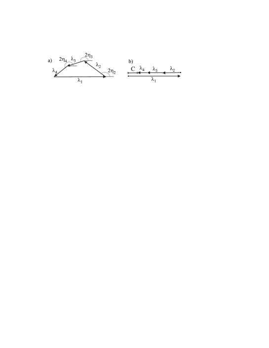
Figure 11: Concurrence polygon: a) quadrangle for a separable state, b) line for an entangled state with concurrence $C$.

Consider now a mixed state $\rho$ for which $C>0$ since $\lambda_{1}$ is so large that the chain cannot be closed – see Fig. 11b. Making use of the pure states $|x_{i}\rangle$ constructed before we introduce a set of four states

$$|y_{1}\rangle=|x_{1}\rangle\ ,\quad|y_{2}\rangle=i|x_{2}\rangle\ ,\quad|y_{3}\rangle=i|x_{3}\rangle\ ,\quad|y_{4}\rangle=i|x_{4}\rangle\ .\quad$$ (93)

and a symmetric matrix $Y_{ij}=\langle y_{i}|{\tilde{y}_{j}}\rangle$, the relative phases of which are chosen in such a way that relation (90) implies

$${\rm Tr}\ Y=\sum_{i=1}^{4}\langle y_{i}|{\tilde{y}_{j}}\rangle=\lambda_{1}-\lambda_{2}-\lambda_{3}-\lambda_{4}\ =\ C(\rho)\ .$$ (94)

The states (93) are subnormalised, hence the above expression represents an average of a real quantity, the absolute value of which coincides with the concurrence (85). Using Schrödinger’s theorem again one may find yet another decomposition, $|z_{i}\rangle\equiv\sum_{i}V^{*}_{ij}|y_{j}\rangle$, such that every state has the same concurrence, $C(|z_{i}\rangle)=C(\rho)$ for $i=1,\dots,4$. To do so define a symmetric matrix $Z_{ij}=\langle z_{i}|{\tilde{z}_{j}}\rangle$ and observe that Tr$Z={\rm Tr}(VYV^{T})$. This trace does not change if $V$ is real and $V^{T}=V^{-1}$ follows. Hence one may find such an orthogonal $V$ that all overlaps are equal to concurrence, $Z_{ii}=C(\rho)$, and produce the final decomposition $\rho=\sum_{i}|z_{i}\rangle\langle z_{i}|$.

The above decomposition is optimal for the concurrence of formation Wo98 ,

$$C_{F}(\rho)\ =\ \min_{{\cal E}_{\rho}}\sum_{i=1}^{M}p_{i}C(|\phi_{i}\rangle)\ =\ \min_{V}\sum_{i=1}^{m}|(VYV^{T})_{ii}|\ ,$$ (95)

where the minimum over ensembles ${\cal E}_{\rho}$ may be replaced by a minimum over $m\times n$ rectangular matrices $V$, containing $n$ orthogonal vectors of size $m\leq 4^{2}$ Uh98 . The function relating $E_{F}$ and concurrence is convex, hence the decomposition into pure states of equal concurrence is also optimal for entropy of formation. Thus $E_{F}$ of any two-qubit state $\rho$ is given by the function (82) of concurrence of formation $C_{F}$ equal to $C(\rho)$, and defined by (89). A streamlined proof of this fact was provided in AVM01 , while the analogous problem for two rebits was solved in CFR02 .

While the algebraic fact i) was used to calculate concurrence, the existence of a general formula for maximal fidelity hinges on property ii). Let us write the state $\rho$ in its Fano form (38) and analyze invariants of local unitary transformations $U_{1}\otimes U_{2}$. Due to the relation $SU(2)\approx SO(3)$ this transformation may be interpreted as an independent rotation of both Bloch vectors, ${\vec{\tau}}^{A}\to O_{1}{\vec{\tau}}^{A}$ and ${\vec{\tau}}^{B}\to O_{2}{\vec{\tau}}^{B}$. Hence the real correlation matrix $\beta_{ij}={\rm Tr}(\rho\sigma_{i}\otimes\sigma_{j})$ may be brought into diagonal form $K=O_{1}\beta O_{2}^{T}$. The diagonal elements may admit negative values since we have restricted orthogonal matrices to fulfill det$O_{i}=+1$. Hence $|K_{ii}|=\kappa_{i}$ where $\kappa_{i}$ stand for singular values of $\beta$. Let us order them decreasingly. By construction they are invariant with respect to local unitaries, and govern the maximal fidelity with respect to maximally entangled states BHHH00 ,

$$F_{m}(\rho)=\frac{1}{4}\bigl{[}1+\kappa_{1}+\kappa_{2}-{\rm Sign}[{\rm det}(\beta)]\ \kappa_{3}\bigr{]}\ .$$ (96)

Two–qubit density matrix is specified by $15$ parameters, the local unitaries are characterized by $6$ variables, so there exist $9$ functionally independent local invariants. However, two states are locally equivalent if they share additional $9$ discrete invariants which determine signs of $\kappa_{i}$, $\tau^{A}_{i}$ and $\tau^{B}_{i}$ Ma02 . A classification of mixed states based on degeneracy and signature of $K$ was worked out in GRB98 ; EM01 ; KZ01 .

It is instructive to compute explicit formulae for above entanglement measures for several families of two–qubit states. The concurrence of a Werner state (42) is equal to the negativity,

$$C\bigl{(}\rho_{W}(x)\bigr{)}={\cal N}_{T}\bigl{(}\rho_{W}(x)\bigr{)}=\left\{\begin{array}[]{ccc}0&{\rm if}&x\leq 1/3\\ (3x-1)/2&{\rm if}&x\geq 1/3\\ \end{array}\right.\ ,$$ (97)

its entanglement of formation is given by (82), while $F_{m}=(3x-1)/4$.

Another interesting family of states arises as a convex combination of a Bell state with an orthogonal separable state HHH00b

$$\sigma_{H}(a)\ \equiv\ a\,|\psi^{-}\rangle\langle\psi^{-}|\ +\ (1-a)\,|00\rangle\langle 00|\ .$$ (98)

Concurrence of such a state is by construction equal to its parameter, $C=a$, while the negativity reads ${\cal N}_{T}=\sqrt{(1-a)^{2}+a^{2}}+a-1$. The relative entanglement of entropy reads VP98 $E_{R}=(a-2)\ln(1-a/2)+(1-a)\ln(1-a)$. We shall use also a mixture of Bell states,

$$\sigma_{B}(b)\ \equiv\ b\,|\psi^{-}\rangle\langle\psi^{-}|+(1-b)\,|\psi^{+}\rangle\langle\psi^{+}|\ ,$$ (99)

for which by construction $F_{m}=\max\{b,1-b\}$ and $C={\cal N}_{T}=2F_{m}-1$.

Entanglement measures are correlated: they vanish for separable states and coincide for maximally entangled states. For two–qubit systems several explicit bounds are known. Concurrence forms an upper bound for negativity EP99 ; Zy99 . This statement was proved in VADM01 , where it was shown that these measures coincide if the eigenvector of $\rho^{T_{A}}$ corresponding to the negative eigenvalue is maximally entangled. The lower bound

$$C\ \geq\ {\cal N}_{T}\ \geq\ \sqrt{(1-C)^{2}+C^{2}}+C-1$$ (100)

is achieved VADM01 for states (98).

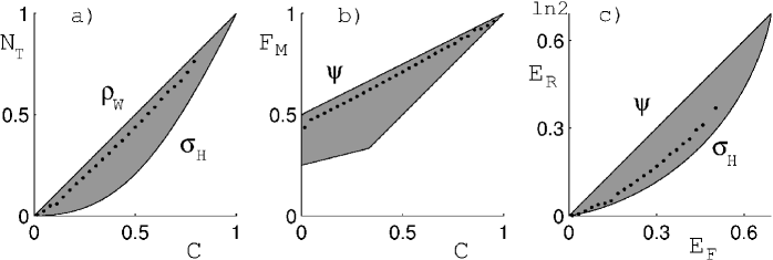
Figure 12: Bounds between entanglement measures for two–qubits: a) negativity versus concurrence (100), b) maximal fidelity versus concurrence (101), c) relative entropy of entanglement versus entanglement of formation (103). Labels represent families of extremal states while dots denote averages taken with respect to the HS measure in ${\cal M}^{(4)}$.

Analogous tight bounds between maximal fidelity and concurrence or negativity were established in VV02b ,

$$\frac{1+C}{2}\geq F_{m}\geq\left\{\begin{array}[]{ccc}(1+C)/4&{\rm if}&C\leq 1/3\\ C&{\rm if}&C\geq 1/3\\ \end{array}\right.\ ,$$ (101)

$$\frac{1+{\cal N}_{T}}{2}\geq F_{m}\geq\left\{\begin{array}[]{ccc}\frac{1}{4}+\frac{1}{8}\Bigl{(}{\cal N}_{T}+\sqrt{5{\cal N}_{T}^{2}+4{\cal N}_{T}}\Bigr{)}&{\rm if}&{\cal N}_{T}\leq\frac{\sqrt{5}-2}{3}\\ \sqrt{2{\cal N}_{T}({\cal N}_{T}+1)}-{\cal N}_{T}&{\rm if}&{\cal N}_{T}\geq\frac{\sqrt{5}-2}{3}\\ \end{array}\right..$$ (102)

Upper bound for fidelity is realized for the family (99) or for any other state for which $C={\cal N}_{T}$.

Relative entropy of entanglement is bounded from above by $E_{F}$. Numerical investigations suggest VADM01 that the lower bound is achieved for the family of (98), which implies

$$E_{F}\geq E_{R}\geq\Bigl{[}(C-2)\ln(1-C/2)+(1-C)\ln(1-C)\Bigr{]}\ .$$ (103)

Here $C^{2}=1-(2\mu_{1}-1)^{2}$ and $\mu_{1}=S^{-1}(E_{F})$ denotes the larger of two preimages of the entropy function (82). Similar bounds between relative entropy of entanglement, and concurrence or negativity were studied in MG04 .

Making use of the analytical formulae for entanglement measures we may try to explore the interior of the $15$-dim set of mixed states. In general, the less quantum state is pure, the less it is entangled: If $R=1/[{\rm Tr}\rho^{2}]\geq 3$ we enter the separable ball and all entanglement measures vanish. Also movements along an global orbit $\rho\to U\rho\,U^{\dagger}$ generically changes entanglement. For a given spectrum $\vec{x}$ the largest concurrence $C^{*}$, which may be achieved on such an orbit is given by Eq. (64) IH00 ; VAM01 . Hence the problem of finding maximally entangled mixed states of two qubits does not have a unique solution: It depends on the measure of mixedness and the measure of entanglement used. Both quantities may be characterised e.g. by a Rényi entropy (or its function), and for each choice of the pair of parameters $q_{1},q_{2}$ one may find an extremal family of mixed states WNGKMV03 .

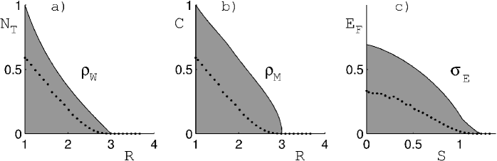
Figure 13: Upper bounds for measures of entanglement as a function of mixedness for two–qubits: a) negativity and b) concurrence versus participation ratio $R=1/({\rm Tr}\rho^{2})$; c) entanglement of formation versus von Neumann entropy. Gray shows entire accessible region while dots denote the average taken with respect to the HS measure in ${\cal M}^{(4)}$. For pure states it coincides with the average over FS measure.

Figure 13 presents average entanglement plotted as a function of measures of mixedness computed with respect to HS measure. For a fixed purity ${\rm Tr}\rho^{2}$ the Werner states (42) produce the maximal negativity ${\cal N}_{T}$. On the other hand, concurrence $C$ becomes maximal for the following states MJWK01

$$\rho_{M}(y)\equiv\left[\begin{array}[]{c c c c}a&0&0&y/2\\ 0&1-2a&0&0\\ 0&0&0&0\\ y/2&0&0&a\end{array}\right],{\ \ \rm where\ \ }\left\{\begin{array}[]{ccc}a=1/3&{\rm if}&y\leq 2/3\\ a=y/2&{\rm if}&y\geq 2/3\\ \end{array}\right.$$ (104)

Here $y\in[0,1]$ and $C(\rho)=y$ while Tr$\rho^{2}=1/3+y^{2}/2$ in the former case and Tr$\rho^{2}=1-2y(1-y)$ in the latter. A family of states $\sigma_{E}$ providing the upper bound of $E_{F}$ as a function of von Neumann entropy (see the line in Fig. 13c) was found in WNGKMV03 . Note that HS measure restricted to pure states coincides with Fubini-Study measure. Hence at $S=0$ the average pure states entropy of entanglement reads $\langle E_{1}\rangle_{\psi}=1/3$ while for $R=1$ we obtain $\langle C\rangle_{\psi}=$ $\langle{\cal N}_{T}\rangle_{\psi}=3\pi/16\approx 0.59$.

Figure 14: Entanglement of formation of generalised Werner states (105) in polar coordinates. White set represents separable states.

To close this section let us show in Fig. 14 entanglement of formation for an illustrative class of two-qubit states

$$\rho(x,\vartheta)\ \equiv\ x(|\psi_{\theta}\rangle\langle\psi_{\theta}|)+(1-x)\rho_{*}{\rm\ \ with\ \ }|\psi_{\theta}\rangle=\frac{1}{\sqrt{2}}\Bigl{(}\sin\frac{\vartheta}{2}|01\rangle+\cos\frac{\vartheta}{2}|10\rangle\Bigr{)}\ .$$ (105)

For $x=1$ the pure state is separable for $\vartheta=0,\pi$ and maximally entangled $(*)$ for $\vartheta=\pi/2,3\pi/2$. The dashed horizontal line represents the Werner states. The set ${\cal M}_{S}$ of separable states contains the maximal ball and touches the set of pure states in two points. A distance $E$ of $\rho$ from the set ${\cal M}_{S}$ may be interpreted as a measure of entanglement.

We have come to the end of our tour across the space of two qubit mixed states. Since all the properties i)-x) break down for higher $N$, the geometry of quantum entanglement gets correspondingly more complex. Already for the system of two qutrits the bound entangled states appear, while the multi-partite problems contain non-equivalent forms of quantum entanglement.

IX Concluding remarks

The aim of this paper is to present literally to present an introduction to the subject of quantum entanglement. Although we have left untouched several important aspects of quantum entanglement, including multipartite systems, infinite dimensional systems, and continuous variables, we hope that a reader may gain a fair overview of basic properties of quantum entanglement.

What is such a knowledge good for? We believe it will contribute to a better understanding of quantum mechanics. We hope also that it will provide a solid foundation for a new, emerging field of science–the theory of quantum information processing. Quantum entanglement plays a decisive role in all branches of the field including quantum cryptography, quantum error correction, and quantum computing.

We would like to thank Johan Brännlund, Åsa Ericsson, Marek Kuś, Florian Mintert and Magdalena Sinołȩcka, with whom we have worked on related projects. We have also enjoyed constructive interactions with Matthias Christandl, Jens Eisert, Michał, Paweł and Ryszard Horodeccy, Vivien Kendon, Artur Łoziński, Christian Schaffner, Paul Slater, and William Wootters.

It is our pleasure to thank for the hospitality at the Perimeter Institute for Theoretical Physics, where this work was done. Financial support by Komitet Badań Naukowych under the grant PBZ-Min-008/P03/03, VW grant ’Entanglement measures and the influence of noise’ and Swedish grant from VR is gratefully acknowledged.

Appendix A Quantum entanglement: Further hints on the literature

The number of papers devoted to quantum entanglement keeps growing fast in the last decade. For instance, 127 papers with the word entanglement or entangled in the title were posted into the archives arXiv during the first quarter of 2006 only. We are not in position to present a review of all the papers which appeared after the book was finished in March 2005. Instead we mention in this appendix some exemplary references, which make our story more complete.

The separability problem for $N\times N$ bi–partite systems remains open for$N\geq 3$. Some spectral conditions implying separability in such systems were provided in Ra06 . Efficient numerical algorithms for detection of separability and entanglement were given in ITCE04 ; HBr04 ; BHH05 .

Valuable recent reviews on entanglement measures are provided by Plenio and Virmani PV05 and Mintert et al. MCKB05 . The monotonicity conditions for entanglement measures have been simplified by M. Horodecki Ho05 , while continuity bounds on the quantum relative entropy were established in AE05 .

The logarithmic negativity was shown to be an entanglement monotone that is not convex Pl05 . Entanglement cost was proved by Yang et al. to be strictly larger than zero for any entangled state YHHSR05 .

Several versions of generalized concurrence for mixed quantum states were investigated in MB05 ; CAF05a ; Go05 ; HBj05 . Entanglement measures for rank-$2$ mixed states where computed by Osborne Os05 , while lower bounds for entanglement of formation of mixed states was found by Chen et al. CAF05b .

Comparative analysis of various entanglement measures and the degree of mixing for two qubit systems was performed in MG04 . Entanglement witnesses for qubits and qutrits were investigated in BDH05 ; JRY05 while an application of witness operators to quantify the entanglement was proposed in Br05 . Relations between entanglement witnesses and Bell inequalities were discussed in HGBL05 .

Properties of the boundary of the set of mixed quantum states and its subset containing separable states were investigated in GKM05 . Later on the set of two qubit separable states was proved to have a constant width SBZ06 . Geometric features of the set of entangled states were analyzed in Le04b ; LMO06 .

Appendix B Contents of the book ”Geometry of Quantum States. An Introduction to Quantum Entanglement” by I. Bengtsson and K. Życzkowski

1 Convexity, colours and statistics

1.1 Convex sets

1.2 High dimensional geometry

1.3 Colour theory

1.4 What is “distance”?

1.5 Probability and statistics

2 Geometry of probability distributions

2.1 Majorization and partial order

2.2 Shannon entropy

2.3 Relative entropy

2.4 Continuous distributions and measures

2.5 Statistical geometry and the Fisher–Rao metric

2.6 Classical ensembles

2.7 Generalized entropies

3 Much ado about spheres

3.1 Spheres

3.2 Parallel transport and statistical geometry

3.3 Complex, Hermitian, and Kähler manifolds

3.4 Symplectic manifolds

3.5 The Hopf fibration of the 3-sphere

3.6 Fibre bundles and their connections

3.7 The 3-sphere as a group

3.8 Cosets and all that

4 Complex projective spaces

4.1 From art to mathematics

4.2 Complex projective geometry

4.3 Complex curves, quadrics and the Segre embedding

4.4 Stars, spinors, and complex curves

4.5 The Fubini-Study metric

4.6 ${\mathbb{C}}{\bf P}^{n}$ illustrated

4.7 Symplectic geometry and the Fubini–Study measure

4.8 Fibre bundle aspects

4.9Grassmannians and flag manifolds

5 Outline of quantum mechanics

5.1 Quantum mechanics

5.2 Qubits and Bloch spheres

5.3 The statistical and the Fubini-Study distances

5.4 A real look at quantum dynamics

5.5 Time reversals

5.6 Classical & quantum states: a unified approach

6 Coherent states and group actions

6.1 Canonical coherent states

6.2 Quasi-probability distributions on the plane

6.3 Bloch coherent states

6.4 From complex curves to $SU(K)$ coherent states

6.5 $SU(3)$ coherent states

7 The stellar representation

7.1 The stellar representation in quantum mechanics

7.2 Orbits and coherent states

7.3 The Husimi function

7.4 Wehrl entropy and the Lieb conjecture

7.5 Generalised Wehrl entropies

7.6 Random pure states

7.7 From the transport problem to the Monge distance

8 The space of density matrices

8.1 Hilbert–Schmidt space and positive operators

8.2 The set of mixed states

8.3 Unitary transformations

8.4 The space of density matrices as a convex set

8.5 Stratification

8.6 An algebraic afterthought

8.7 Summary

9 Purification of mixed quantum states

9.1 Tensor products and state reduction

9.2 The Schmidt decomposition

9.3 State purification & the Hilbert-Schmidt bundle

9.4 A first look at the Bures metric

9.5 Bures geometry for $N=2$

9.6 Further properties of the Bures metric

10 Quantum operations

10.1 Measurements and POVMs

10.2 Algebraic detour: matrix reshaping and reshuffling

10.3 Positive and completely positive maps

10.4 Environmental representations

10.5 Some spectral properties

10.6 Unital & bistochastic maps

10.7 One qubit maps

11 Duality: maps versus states

11.1 Positive & decomposable maps

11.2 Dual cones and super-positive maps

11.3 Jamiołkowski isomorphism

11.4 Quantum maps and quantum states

12 Density matrices and entropies

12.1 Ordering operators

12.2 Von Neumann entropy

12.3 Quantum relative entropy

12.4 Other entropies

12.5 Majorization of density matrices

12.6 Entropy dynamics

13 Distinguishability measures

13.1 Classical distinguishability measures

13.2 Quantum distinguishability measures

13.3 Fidelity and statistical distance

14 Monotone metrics and measures

14.1 Monotone metrics

14.2 Product measures and flag manifolds

14.3 Hilbert-Schmidt measure

14.4 Bures measure

14.5 Induced measures

14.6 Random density matrices

14.7 Random operations

15 Quantum entanglement

15.1 Introducing entanglement

15.2 Two qubit pure states: entanglement illustrated

15.3 Pure states of a bipartite system

15.4 Mixed states and separability

15.5 Geometry of the set of separable states

15.6 Entanglement measures

15.7 Two qubit mixed states

Epilogue

Appendix 1 Basic notions of differential geometry

Appendix 2 Basic notions of group theory

Appendix 3 Geometry do it yourself

Appendix 4 Hints and answers to the exercises

Appendix C  Geometry—do it yourself

In this appendix we provide some additional exercises of a more practical nature. Working them out might improve our skills and intuition required to cope with multi-dimensional geometric objects which arise while investigating quantum entanglement.

Exercise 1 – Real projective space. Cut out a disk of radius $r$. Prepare a narrow strip of length $\pi r$ and glue it into a Möbius strip. The total length of the boundary of a strip is equal to the circumference of the disk so you may try to glue them together. (If you happen to work in $3$ dimensions this simple task gets difficult…) If you are done, you can contemplate a nice model of a real projective space, ${\mathbbm{R}}{\bf P}^{2}$.

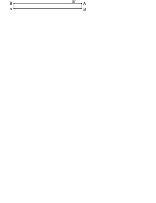
Figure 15: A narrow Möbius strip glued with a circle produces ${\mathbb{R}}{\bf P}^{2}$.

Exercise 2 – Hypersphere ${\bf S}^{3}$ may be obtained by identifying points on the surfaces of two identical $3$–balls as discussed in section 3.3 To experience further features of the hypersphere get some playdough and prepare two cylinders of different colours with their length more than three times larger than their diameter. Form two linked tori as shown in Fig. 16.

Start gluing them together along their boundaries. After this procedure (not easy in 3-D) is completed you will be in position to astonish your colleagues by presenting them a genuine Heegard decomposition of a hypersphere.

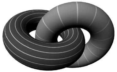
Figure 16: Heegard decomposition of a three–sphere.

Exercise 3 – Entangled pure states. Magnify Fig. 17 and cut out the net of the cover tetrahedron. It represents the entanglement of formation of the pure states of two qubits for a cross-section of ${\mathbb{C}}{\bf P}^{3}$.

Glue it together to get the entanglement tetrahedron with four product states in four corners. Enjoy the symmetry of the object and study the contours of the states of equal entanglement.

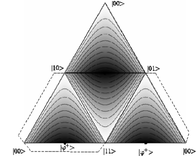
Figure 17: Net of the tetrahedron representing entanglement for pure states of two qubits: maximally entangled states plotted in black.

Exercise 4 – Separable pure states. Prepare a net of a regular tetrahedron from transparency according to the blueprint shown in Fig. 18. Make holes with a needle along two opposite edges as shown in the picture. Thread a needle with a (red) thread and start sewing it through your model. Only after this job is done glue the tetrahedron together. (Our practice shows that sewing after the tetrahedron is glued together is much more difficult…) If you pull out the loose tread and get the object sketched in Fig. 1, you can contemplate, how a fragment of the subspace of separable states forms a ruled surface embedded inside the tetrahedron.

Figure 18: Sew with a colour thread inside a transparent tetrahedron to get the ruled surface consisting of separable pure states of two qubits.

References

- (1) S. Abe and A. K. Rajagopal. Nonadditive conditional entropy and its significance for local realism. Physica, A 289:157, 2001.
- (2) A. Acín, A. Andrianov, E. Jané, and R. Tarrach. Three–qubit pure state canonical forms. J. Phys., A 34:6725, 2001.
- (3) S. J. Akhtarshenas and M. A. Jafarizadeh. Robustness of entanglement for Bell decomposable states. E. Phys. J., D 25:293, 2003.
- (4) S. J. Akhtarshenas and M. A. Jafarizadeh. Optimal Lewenstein-Sanpera decomposition for some bipartite systems. J. Phys., A 37:2965, 2004.
- (5) S. Albeverio, K. Chen, and S.-M. Fei. Generalized reduction criterion for separability of quantum states. Phys. Rev., A 68:062313, 2003.
- (6) R. Alicki and M. Fannes. Continuity of quantum conditional information. J. Phys., A 37:L55, 2004.
- (7) N. Alon and L. Lovasz. Unextendible product bases. J. Combinat. Theor., A 95:169, 2001.
- (8) P. Aravind. The ”twirl”, stella octangula and mixed state entanglement. Phys. Lett., A 233:7, 1997.
- (9) M. Asoudeh, V. Karimipour, L. Memarzadeh, and A. T. Rezakhani. On a suggestion relating topological and quantum mechanical entanglements. Phys. Lett., A 327:380, 2004.
- (10) A. Aspect, J. Dalibard, and G. Roger. Experimental test of Bell’s inequalities using time-varying analysers. Phys. Rev. Lett., 49:1804, 1982.
- (11) K. Audenaert and J. Eisert. Continuity bounds on the quantum relative entropy. J. Math. Phys., 46:102104, 2005.
- (12) K. Audenaert, J. Eisert, E. Jané, M. B. Plenio, S. Virmani, and B. D. Moor. Asymptotic relative entropy of entanglement. Phys. Rev. Lett., 87:217902, 2001.
- (13) K. Audenaert, B. D. Moor, K. G. H. Vollbrecht, and R. F. Werner. Asymptotic relative entropy of entanglement for orthogonally invariant states. Phys. Rev., A 66:032310, 2002.
- (14) K. Audenaert, F. Verstraete, and B. D. Moor. Variational characterizations of separability and entanglement of formation. Phys. Rev., A 64:052304, 2001.
- (15) P. Badzia̧g, P. Deaur, M. Horodecki, P. Horodecki, and R. Horodecki. Concurrence in arbitrary dimensions. J. Mod. Optics, 49:1289, 2002.
- (16) P. Badzia̧g, M. Horodecki, P. Horodecki, and R. Horodecki. Local environment can enhance fidelity of quantum teleportation. Phys. Rev., A 62:012311, 2000.
- (17) P. Badzia̧g, P. Horodecki, and R. Horodecki. Towards efficient algorithm deciding separability of distributed quantum states. Preprint quant-ph/0504041.
- (18) S. Bandyopadhyay and V. Roychowdhury. Supercatalysis. Phys. Rev., A 65:042306, 2002.
- (19) M. Barbieri, F. D. Martini, G. D. Nepi, P. Mataloni, G. D’Ariano, and C. Macciavello. Detection of entanglement with polarized photons: Experimental realization of an entanglement witness. Phys. Rev. Lett., 91:227901, 2003.
- (20) H. Barnum, E. Knill, G. Ortiz, and L. Viola. Generalizations of entanglement based on coherent states and convex sets. Phys. Rev., A 68:032308, 2003.
- (21) J. Batle, A. R. Plastino, M. Casas, and A. Plastino. Inclusion relations among separability criteria. J. Phys., A 37:895, 2004.
- (22) J. S. Bell. On the Einstein Podolsky Rosen paradox. Physics, 1:195, 1964.
- (23) J. S. Bell. Speakable and Unspeakable in Quantum Mechanics. Cambridge University Press, Cambridge, 1987.
- (24) F. Benatti, R. Floreanini, and M. Piani. Quantum dynamical semigroups and non-decomposable positive maps. Phys. Lett., A 326:187, 2004.
- (25) F. Benatti and H. Narnhofer. Additivity of the entanglement of formation. Phys. Rev., A 63:042306, 2001.
- (26) I. Bengtsson, J. Brännlund, and K. Życzkowski. , or entanglement illustrated. Int. J. Mod. Phys., A 17:4675, 2002.
- (27) I. Bengtsson and K. Życzkowski. Geometry of Quantum States. An Introduction to Quantum Entanglement. Cambridge University Press, 2006.
- (28) C. H. Bennett, H. J. Bernstein, S. Popescu, and B. Schumacher. Concentrating partial entanglement by local operations. Phys. Rev., A 53:2046, 1996.
- (29) C. H. Bennett, G. Brassard, C. Crépeau, R. Josza, A. Peres, and W. K. Wootters. Teleporting an unknown quantum state via dual classical and Einstein–Podolsky–Rosen channels. Phys. Rev. Lett., 70:1895, 1993.
- (30) C. H. Bennett, D. P. DiVincenzo, C. A. Fuchs, T. Mor, E. Rains, P. W. Shor, J. A. Smolin, and W. K. Wootters. Quantum nonlocality without entanglement. Phys. Rev., A 59:1070, 1999.
- (31) C. H. Bennett, D. P. DiVincenzo, T. Mor, P. W. Shor, J. A. Smolin, and B. M. Terhal. Unextendible product bases and bound entanglement. Phys. Rev. Lett., 82:5385, 1999.
- (32) C. H. Bennett, D. P. DiVincenzo, J. Smolin, and W. K. Wootters. Mixed-state entanglement and quantum error correction. Phys. Rev., A 54:3824, 1996.
- (33) C. H. Bennett, S. Popescu, D. Rohrlich, J. A. Smolin, and A. V. Thapliyal. Exact and asymptotic measures of multipartite pure-state entanglement. Phys. Rev., A 63:012307, 2001.
- (34) B. A. Bernevig and H. D. Chen. Geometry of the 3-qubit state, entanglement and division algebras. J. Phys., A 36:8325, 2003.
- (35) R. Bertlmann, K. Durstberger, and B. C. Hiesmayr. Optimal entanglement witnesses for qubits and qutrits. Phys. Rev., A 72:052331, 2005.
- (36) P. Blanchard, L. Jakóbczyk, and R. Olkiewicz. Measures of entanglement based on decoherence. J. Phys., A 34:8501, 2001.
- (37) D. Boschi, S. Branca, F. De Martini, L. Hardy, and S. Popescu. Experimental realization of teleporting an unknown pure quantum state via dual classical and Einstein-Podolsky-Rosen channels. Phys. Rev. Lett., 80:1121, 1998.
- (38) J. Bouda and V. Bužek. Purification and correlated measurements of bipartite mixed states. Phys. Rev., A 65:034304, 2002.
- (39) M. Bourennane, M. Eibl, C. Kurtsiefer, H. Weinfurter, O. Guehne, P. Hyllus, D. Bruß, M. Lewenstein, and A. Sanpera. Witnessing multipartite entanglement. Phys. Rev. Lett., 92:087902, 2004.
- (40) D. Bouwmeester, J.-W. Pan, K. Mattle, M. Eibl, H. Weinfurter, and A. Zeilinger. Experimental quantum teleportation. Nature, 390:575, 1997.
- (41) F. Brandao. Quantifying entanglement with witness operators. Phys. Rev., A 72:022310, 2005.
- (42) S. L. Braunstein, C. M. Caves, R. Jozsa, N. Linden, S. Popescu, and R. Schack. Separability of very noisy mixed states and implications for NMR quantum computing. Phys. Rev. Lett., 83:1054, 1999.
- (43) G. K. Brennen. An observable measure of entanglement for pure states of multi-qubit systems. Quant. Inf. Comp., 3:619, 2003.
- (44) D. C. Brody and L. P. Hughston. Geometric quantum mechanics. J. Geom. Phys., 38:19, 2001.
- (45) T. A. Brun and O. Cohen. Parametrization and distillability of three-qubit entanglement. Phys. Lett., A 281:88, 2001.
- (46) D. Bruß. Characterizing entanglement. J. Math. Phys., 43:4237, 2002.
- (47) D. Bruß, J. I. Cirac, P. Horodecki, F. Hulpke, B. Kraus, M. Lewenstein, and A. Sanpera. Reflections upon separability and distillability. J. Mod. Opt., 49:1399, 2002.
- (48) D. Bruß and A. Peres. Construction of quantum states with bound entanglement. Phys. Rev., A 61:30301(R), 2000.
- (49) H. A. Carteret, A. Higuchi, and A. Sudbery. Multipartite generalisation of the Schmidt decomposition. J. Math. Phys., 41:7932, 2000.
- (50) C. M. Caves, C. A. Fuchs, and P. Rungta. Entanglement of formation of an arbitrary state of two rebits. Found. Phys. Lett., 14:199, 2001.
- (51) N. J. Cerf and C. Adami. Quantum extension of conditional probability. Phys.Rev., A 60:893, 1999.
- (52) N. J. Cerf, C. Adami, and R. M. Gingrich. Reduction criterion for separability. Phys. Rev., A 60:898, 1999.
- (53) K. Chen, S. Albeverio, and S.-M. Fei. Concurrence of arbitrary dimensional bipartite quantum states. Phys. Rev. Lett., 95:040504, 2005.
- (54) K. Chen, S. Albeverio, and S.-M. Fei. Entanglement of formation of bipartite quantum states. Phys. Rev. Lett., 95:210501, 2005.
- (55) K. Chen and L.-A. Wu. The generalized partial transposition criterion for separability of multipartite quantum states. Phys. Lett., A 306:14, 2002.
- (56) K. Chen and L.-A. Wu. A matrix realignment method for recognizing entanglement. Quant. Inf. Comp., 3:193, 2003.
- (57) K. Chen and L.-A. Wu. Test for entanglement using physically observable witness operators and positive maps. Phys. Rev., A 69:022312, 2004.
- (58) P.-X. Chen, L.-M. Liang, C.-Z. Li, and M.-Q. Huang. A lower bound on entanglement of formation of system. Phys. Lett., A 295:175, 2002.
- (59) I. L. Chuang, N. Gershenfeld, M. G. Kubinec, and D. W. Leung. Bulk quantum computation with nuclear magnetic resonance: theory and experiment. Proc. Royal Soc. London. Ser. A, 454:447, 1998.
- (60) J. F. Clauser and A. Shimony. Bell’s theorem; experimental tests and implications. Rep. Prog. Phys., 41:1881, 1978.
- (61) R. Clifton and H. Halvorson. Bipartite mixed states of infinite-dimensional systems are generically nonseparable. Phys. Rev., A 61:012108, 2000.
- (62) R. Clifton, B. Hepburn, and C. Wuthrich. Generic incomparability of infinite-dimensional entangled states. Phys. Lett., A 303:121, 2002.
- (63) V. Coffman, J. Kundu, and W. K. Wootters. Distributed entanglement. Phys. Rev., A 61:052306, 2000.
- (64) D. Collins and S. Popescu. Classical analog of entanglement. Phys. Rev., A 65:032321, 2002.
- (65) D. G. Cory, A. F. Fahmy, and T. F. Havel. Ensemble quantum computing by NMR spectroscopy. Proc. Natl. Acad. Sci. USA, 94:1634, 1997.
- (66) S. Daftuar and M. Klimesh. Mathematical structure of entanglement catalysis. Phys. Rev., A 64:042314, 2001.
- (67) P. Deuar, W. J. Munro, and K. Nemoto. Upper bound on the region of separable states near the maximally mixed state. J. Opt., B 2:225, 2000.
- (68) I. Devetak and A. Winter. Distillation of secret key and entanglement from quantum states. Proc. Royal Soc. Lond. A Math.-Phys., 461:207, 2005.
- (69) D. DiVincenzo, C. A. Fuchs, H. Mabuchi, J. A. Smolin, A. Thapliyal, and A. Uhlmann. Entanglement of assistance. Lecture Notes Comp. Sci., 1509:247, 1999.
- (70) D. DiVincenzo, B. Terhal, and A. V. Thapliyal. Optimal decompositions of barely separable states. J. Mod. Opt., 47:377, 2000.
- (71) D. P. DiVincenzo, T. Mor, P. W. Shor, J. A. Smolin, and B. M. Terhal. Unextendible product bases, uncompletable product bases and bound entanglement. Comm. Math. Phys., 238:379, 2003.
- (72) D. P. DiVincenzo, P. W. Shor, J. A. Smolin, B. M. Terhal, and A. Thapliyal. Evidence for bound entangled states with negative partial transpose. Phys. Rev., A 61:062312, 2000.
- (73) A. C. Doherty, P. A. Parillo, and F. M. Spedalieri. Distinguishing separable and entangled states. Phys. Rev. Lett., 88:187904, 2002.
- (74) A. C. Doherty, P. A. Parillo, and F. M. Spedalieri. Complete family of separability criteria. Phys. Rev., A 69:022308, 2004.
- (75) M. J. Donald and M. Horodecki. Continuity of relative entropy of entanglement. Phys. Lett., A 264:257, 1999.
- (76) M. J. Donald, M. Horodecki, and O. Rudolph. The uniqueness theorem for entanglement measures. J. Math. Phys., 43:4252, 2002.
- (77) W. Dür, J. I. Cirac, M. Lewenstein, and D. Bruß. Distillability and partial transposition in bipartite systems. Phys. Rev., A 61:062313, 2000.
- (78) W. Dür, G. Vidal, and J. I. Cirac. Three qubits can be entangled in two inequivalent ways. Phys. Rev., A 62:062314, 2000.
- (79) T. Eggeling, K. Vollbrecht, R. Werner, and M. Wolf. Distillability via protocols respecting the positivity of partial transpose. Phys. Rev. Lett., 87:257902, 2001.
- (80) A. Einstein. Autobiographical Notes. In P. A. Schilpp, editor, Albert Einstein: Philosopher – Scientist, page 1. Cambridge University Press, Cambridge, 1949.
- (81) A. Einstein, B. Podolsky, and N. Rosen. Can quantum mechanical description of reality be considered complete ? Phys. Rev., 47:777, 1935.
- (82) J. Eisert. Entanglement in Quantum Information Theory. Ph.D. Thesis, University of Potsdam, 2001.
- (83) J. Eisert, K. Audenaert, and M. B. Plenio. Remarks on entanglement measures and non-local state distinguishability. J. Phys., A 36:5605, 2003.
- (84) J. Eisert and H. J. Briegel. Schmidt measure as a tool for quantifying multiparticle entanglement. Phys. Rev., A 64:022306, 2001.
- (85) J. Eisert, P. Hyllus, O. Guhne, and M. Curty. Complete hierarchies of efficient approximations to problems in entanglement theory. Phys. Rev., A 70:062317, 2004.
- (86) J. Eisert and M. B. Plenio. A comparison of entanglement measures. J. Mod. Opt., 46:145, 1999.
- (87) B.-G. Englert and N. Metwally. Remarks on –q-bit states. Appl. Phys., B 72:35, 2001.
- (88) A. Ericsson. Separability and the stella octangula. Phys. Lett., A 295:256, 2002.
- (89) H. Everett. ”Relative state” formulation of quantum mechanics. Rev. Mod. Phys., 29:454, 1957.
- (90) U. Fano. Pairs of two–level systems. Rev. Mod. Phys., 55:855, 1983.
- (91) E. Gerjuoy. Lower bound on entanglement of formation for the qubit-qudit system. Phys. Rev., A 67:052308, 2003.
- (92) R. Gill. Time, finite statistics, and Bell’s fifth position. In A. Khrennikov, editor, Foundations of Probability and Physics – 2, page 179. Växjö UP, 2003.
- (93) R. M. Gingrich. Properties of entanglement monotones for three–qubit pure states. Phys. Rev., A 65:052302, 2002.
- (94) G. Gour. Mixed-state entanglement of assistance and the generalized concurrence. Phys. Rev., A 72:042318, 2005.
- (95) M. Grassl, M. Rötteler, and T. Beth. Computing local invariants of qubit systems. Phys. Rev., A 58:1833, 1998.
- (96) D. M. Greenberger, M. Horne, and A. Zeilinger. Going beyond Bell’s theorem. In M. Kafatos, editor, Bell’s Theorem, Quantum Theory and Conceptions of the Universe, page 69. Kluver, Dordrecht, 1989.
- (97) O. Gühne, P. Hyllus, D. Bruß, A. Ekert, M. Lewenstein, C. Macchiavello, and A. Sanpera. Experimental detection of entanglement via witness operators and local measurements. J. Mod. Opt., 50:1079, 2003.
- (98) O. Gühne and M. Lewenstein. Entropic uncertainty relations and entanglement. Phys. Rev., A 70:022316, 2004.
- (99) L. Gurvits. Classical deterministic complexity of Edmonds’ problem and quantum entanglement. In Proceedings of the 35-th ACM Symposium on Theory of Computing, page 10. ACM Press, New York, 2003.
- (100) L. Gurvits. Classical complexity and quantum entanglement. J. Comput. Syst. Sciences, 69:448, 2004.
- (101) L. Gurvits and H. Barnum. Largest separable balls around the maximally mixed bipartite quantum state. Phys. Rev., A 66:062311, 2002.
- (102) L. Gurvits and H. Barnum. Separable balls around the maximally mixed multipartite quantum states. Phys. Rev., A 68:042312, 2003.
- (103) L. Gurvits and H. Barnum. Further results on the multipartite separable ball. quant-ph, 04:09095, 2004.
- (104) K.-C. Ha, S.-H. Kye, and Y.-S. Park. Entangled states with positive partial transposes arising from indecomposable positive linear maps. Phys. Lett., A 313:163, 2003.
- (105) L. Hardy. Method of areas for manipulating the entanglement properties of one copy of a two-particle pure entangled state. Phys. Rev., A 60:1912, 1999.
- (106) P. Hayden, B. M. Terhal, and A. Uhlmann. On the LOCC classification of bipartite density matrices. Preprint quant-ph/0011095.
- (107) P. M. Hayden, M. Horodecki, and B. M. Terhal. The asymptotic entanglement cost of preparing a quantum state. J. Phys., A 34:6891, 2001.
- (108) M. Hein, J. Eisert, and H. J. Briegel. Multiparty entanglement in graph states. Phys. Rev., A 69:062311, 2004.
- (109) L. Henderson and V. Vedral. Information, relative entropy of entanglement and irreversibility. Phys. Rev. Lett., 84:2263, 2000.
- (110) H. Heydari and G. Bjork. Entanglement measure for general pure multipartite quantum states. J. Phys., A 37:9251, 2004.
- (111) H. Heydari and G. Bjork. Entanglement measure for pure bipartite quantum states. Opt. Spectrosc., 99:379, 2005.
- (112) R. Hildebrand. PPT from spectra. Preprint quant-ph/0502170.
- (113) S. Hill and W. K. Wootters. Entanglement of a pair of quantum bits. Phys. Rev. Lett., 78:5022, 1997.
- (114) K. Horodecki, M. Horodecki, P. Horodecki, and J. Oppenheim. Secure key from bound entanglement. Preprint quant-ph/0309110.
- (115) M. Horodecki. Entanglement measures. Quant. Inf. Comp., 1:3, 2001.
- (116) M. Horodecki. Simplifying monotonicity conditions for entanglement measures. Open Sys. & Infor. Dyn., 12:231, 2005.
- (117) M. Horodecki and P. Horodecki. Reduction criterion of separability and limits for a class of distillation protocols. Phys. Rev., A 59:4206, 1999.
- (118) M. Horodecki, P. Horodecki, and R. Horodecki. Separability of mixed states: necessary and sufficient conditions. Phys. Lett., A 223:1, 1996.
- (119) M. Horodecki, P. Horodecki, and R. Horodecki. Mixed-state entanglement and distillation: is there a “bound” entanglement in nature? Phys. Rev. Lett., 80:5239, 1998.
- (120) M. Horodecki, P. Horodecki, and R. Horodecki. Limits for entanglement measures. Phys. Rev. Lett., 84:2014, 2000.
- (121) M. Horodecki, P. Horodecki, and R. Horodecki. Mixed–state entanglement and quantum communication. In G. Alber and M. Weiner, editors, Quantum Information – Basic Concepts and Experiments, page 1. Springer, Berlin, 2000.
- (122) M. Horodecki, P. Horodecki, and R. Horodecki. Separability of mixed quantum states: Linear contractions and permutation criteria. Open Sys. & Infor. Dyn., 13:103, 2006.
- (123) M. Horodecki, P. W. Shor, and M. B. Ruskai. Entanglement breaking channels. Rev. Math. Phys., 15:621, 2003.
- (124) P. Horodecki. Separability criterion and inseparable mixed states with positive partial transposition. Phys. Lett., A 232:333, 1997.
- (125) P. Horodecki, M. Horodecki, and R. Horodecki. Bound entanglement can be activated. Phys. Rev. Lett., 82:1056, 1999.
- (126) P. Horodecki, M. Lewenstein, G. Vidal, and I. Cirac. Operational criterion and constructive checks for the separability of low rank density matrices. Phys. Rev., A 62:032310, 2000.
- (127) P. Horodecki, J. A. Smolin, B. M. Terhal, and A. V. Thapliyal. Rank two bipartite bound entangled states do not exist. Theor. Comp. Sci., 292:589, 2003.
- (128) R. Horodecki and M. Horodecki. Information-theoretic aspects of quantum inseparability of mixed states. Phys. Rev., A 54:1838, 1996.
- (129) R. Horodecki and P. Horodecki. Quantum redundancies and local realism. Phys. Lett., A 194:147, 1994.
- (130) R. Horodecki, P. Horodecki, and M. Horodecki. Quantum -entropy inequalities: independent condition for local realism? Phys. Lett., A 210:377, 1996.
- (131) F. Hulpke and D. Bruß. A two-way algorithm for the entanglement problem. J. Phys., A 38:5573, 2005.
- (132) P. Hyllus, O. Gühne, D. Bruß, and M. Lewenstein. Relations between entanglement witnesses and Bell inequalities. Phys. Rev., A 72:023421, 2005.
- (133) L. Ioannou, B. C. Travaglione, D. Cheung, and A. K. Ekert. Improved algorithm for quantum separability and entanglement detection. Phys. Rev., A 70:060303, 2004.
- (134) S. Ishizaka. Analytical formula connecting entangled state and the closest disentangled state. Phys. Rev., A 67:060301, 2003.
- (135) S. Ishizaka and T. Hiroshima. Maximally entangled mixed states under nonlocal unitary operations in two qubits. Phys. Rev., A 62:022310, 2000.
- (136) M. A. Jafarizadeh, M. Rezaee, and S. Yagoobi. Bell-state diagonal-entanglement witnesses. Phys. Rev., A 72:062106, 2005.
- (137) L. Jakóbczyk and M. Siennicki. Geometry of Bloch vectors in two–qubit system. Phys. Lett., A 286:383, 2001.
- (138) J. G. Jensen and R. Schack. A simple algorithm for local conversion of pure states. Phys. Rev., A 63:062303, 2001.
- (139) D. Jonathan and M. B. Plenio. Entanglement–assisted local manipulation of pure quantum states. Phys. Rev. Lett., 83:3566, 1999.
- (140) D. Jonathan and M. B. Plenio. Minimial conditions for local pure-state entanglement manipulation. Phys. Rev. Lett., 83:1455, 1999.
- (141) R. Jozsa, D. Robb, and W. K. Wootters. Lower bound for accessible information in quantum mechanics. Phys. Rev., A 49:668, 1994.
- (142) S. Karnas and M. Lewenstein. Separable approximations of density matrices of composite quantum systems. J. Phys., A 34:6919, 2001.
- (143) L. H. Kauffmann and S. J. Lomonaco Jr. Comparing quantum entanglement and topological entanglement. New. J. Phys., 4:73.1, 2002.
- (144) V. M. Kendon, K. Życzkowski, and W. J. Munro. Bounds on entanglement in qudit subsystems. Phys. Rev., A 66:062310, 2002.
- (145) M. Kuś and K. Życzkowski. Geometry of entangled states. Phys. Rev., A 63:032307, 2001.
- (146) R. Laflamme, D. Cory, C. Negrevergne, and L. Viola. NMR quantum information processing and entanglement. Quantum Inform. Compu., 2:166, 2002.
- (147) S. Lee, D. P. Chi, S. D. Oh, and J. Kim. Convex-roof extended negativity as an entanglement measure for bipartite quantum systems. Phys. Rev., A 68:062304, 2003.
- (148) J. M. Leinaas, J. Myrheim, and E. Ovrum. Geometrical aspects of entanglement. Preprint quant-ph/0605079.
- (149) P. Lévay. The geometry of entanglement: metrics, connections and the geometric phase. J. Phys., A 37:1821, 2004.
- (150) M. Lewenstein, D. Bruß, J. I. Cirac, B. Kraus, M. Kuś, J. Samsonowicz, A. Sanpera, and R. Tarrach. Separability and distillability in composite quantum systems – a primer. J. Mod. Opt., 47:2841, 2000.
- (151) M. Lewenstein, B. Kraus, J. I. Cirac, and P. Horodecki. Optimization of entanglement witnesses. Phys. Rev., A 62:052310, 2000.
- (152) M. Lewenstein and A. Sanpera. Separability and entanglement of composite quantum systems. Phys. Rev. Lett., 80:2261, 1998.
- (153) H.-K. Lo and S. Popescu. Concentrating entanglement by local actions: Beyond mean values. Phys. Rev., A 63:022301, 1998.
- (154) R. Lockhart. Optimal ensemble length of mixed separable states. J. Math. Phys., 41:6766, 2000.
- (155) R. B. Lockhart and M. J. Steiner. Preserving entanglement under perturbation and sandwiching all separable states. Phys. Rev., A 65:022107, 2002.
- (156) R. B. Lockhart, M. J. Steiner, and K. Gerlach. Geometry and product states. Quant. Inf. Comp., 2:333, 2002.
- (157) A. Łoziński, A. Buchleitner, K. Życzkowski, and T. Wellens. Entanglement of quantum systems. Europhys. Lett., A 62:168, 2003.
- (158) H. Maassen and J. B. M. Uffink. Generalized entropic uncertainty relations. Phys. Rev. Lett., 60:1103, 1988.
- (159) Y. Makhlin. Nonlocal properties of two-qubit gates and mixed states, and the optimization of quantum computations. Quant. Inf. Proc., 1:243, 2002.
- (160) M. L. Mehta. Matrix Theory. Hindustan Publishing, Delhi, 1989.
- (161) D. A. Meyer and N. R. Wallach. Global entanglement in multiparticle systems. J. Math. Phys., 43:4273, 2002.
- (162) F. Mintert and A. Buchleitner. Concurrence of quasipure quantum states. Phys. Rev., A 72:012336, 2005.
- (163) F. Mintert, A. Carvalho, M. Kuś, and A. Buchleitner. Measures and dynamics of entangled states. Phys. Rep., 415:207, 2005.
- (164) F. Mintert, M. Kuś, and A. Buchleitner. Concurrence of mixed bipartite quantum states in arbitrary dimensions. Phys. Rev. Lett., 92:167902, 2004.
- (165) F. Mintert and K. Życzkowski. Wehrl entropy, Lieb conjecture and entanglement monotones. Phys. Rev., A 69:022317, 2004.
- (166) A. Miranowicz and A. Grudka. A comparative study of relative entropy of entanglement, concurrence and negativity. J. Opt. B: Quantum Semiclass. Opt., 6:542, 2004.
- (167) A. Miyake. Classification of multipartite entangled states by multidimensional determinants. Phys. Rev., A 67:012108, 2003.
- (168) J. M.Kuś and G. Marmo. Geometry of quantum systems: density states and entanglement. J. Phys., A 38:10217, 2005.
- (169) R. Mosseri and R. Dandoloff. Geometry of entangled states, Bloch spheres and Hopf fibrations. J. Phys., A 34:10243, 2001.
- (170) W. J. Munro, D. F. V. James, A. G. White, and P. G. Kwiat. Maximizing the entanglement of two mixed qubits. Phys. Rev., A 64:030302, 2001.
- (171) M. A. Nielsen. Conditions for a class of entanglement transformations. Phys. Rev. Lett., 83:436, 1999.
- (172) M. A. Nielsen. Continuity bounds for entanglement. Phys. Rev., A 61:064301, 2000.
- (173) M. A. Nielsen and J. Kempe. Separable states are more disordered globally than locally. Phys. Rev. Lett., 86:5184, 2001.
- (174) K. M. O’Connor and W. K. Wootters. Entangled rings. Phys. Rev., A 63:052302, 2001.
- (175) T. J. Osborne. Entanglement measure for rank- mixed states. Phys. Rev., A 72:022309, 2005.
- (176) M. Ozawa. Entanglement measures and the Hilbert-Schmidt distance. Phys. Lett., A 268:158, 2001.
- (177) M. H. Partovi. Universal measure of entanglement. Phys. Rev. Lett., 92:077904, 2004.
- (178) A. Peres. Higher order Schmidt decomposition. Phys. Lett., A202:16, 1995.
- (179) A. Peres. Separability criterion for density matrices. Phys. Rev. Lett., 77:1413, 1996.
- (180) D. Petz. Monotone metrics on matrix spaces. Linear Algebra Appl., 244:81, 1996.
- (181) A. O. Pittenger. Unextendible product bases and the construction of inseparable states. Linear Albegra Appl., 359:235, 2003.
- (182) A. O. Pittenger and M. H. Rubin. Separability and Fourier representations of density matrices. Phys. Rev., A 62:032313, 2000.
- (183) A. O. Pittenger and M. H. Rubin. Convexity and the separability problem of quantum mechanical density matrices. Linear Algebra Appl., 346:47, 2002.
- (184) A. O. Pittenger and M. H. Rubin. Geometry of entanglement witnesses and local detection of entanglement. Phys. Rev., A 67:012327, 2003.
- (185) M. B. Plenio. Logarithmic negativity: A full entanglement monotone that is not convex. Phys. Rev. Lett., 95:090503, 2005.
- (186) M. B. Plenio and S. Virmani. An introduction to entanglement measures. Preprint quant-ph/0504163.
- (187) M. Plesch and V. Bužek. Entangled graphs: Bipartite entanglement in multiqubit systems. Phys. Rev., A 67:012322, 2003.
- (188) S. Popescu and D. Rohrlich. Thermodynamics and the measure of entanglement. Phys. Rev., A 56:R3319, 1997.
- (189) G. Raggio. Spectral conditions on the state of a composite quantum system implying its separability. J. Phys., A 39:617, 2006.
- (190) E. M. Rains. Bound on distillable entanglement. Phys. Rev., A 60:179, 1999.
- (191) E. M. Rains. Rigorous treatment of distillable entanglement. Phys. Rev., A 60:173, 1999.
- (192) E. M. Rains. A semidefinite program for distillable entanglement. IEEE Trans. Inform. Theory, 47:2921, 2001.
- (193) A. K. Rajagopal and R. W. Rendell. Separability and correlations in composite states based on entropy methods. Phys. Rev., A 66:022104, 2002.
- (194) J. Řeháček and Z. Hradil. Quantification of entanglement by means of convergent iterations. Phys. Rev. Lett., 90:127904, 2003.
- (195) R. Rossignoli and N. Canosa. Generalized entropic criterion for separability. Phys. Rev., A 66:042306, 2002.
- (196) O. Rudolph. A new class of entanglement measures. J. Math. Phys., A 42:5306, 2001.
- (197) O. Rudolph. On the cross norm criterion for separability. J. Phys., A 36:5825, 2003.
- (198) O. Rudolph. Some properties of the computable cross norm criterion for separability. Physical Review, A 67:032312, 2003.
- (199) P. Rungta, V. Bužek, C. M. Caves, M. Hillery, and G. J. Milburn. Universal state inversion and concurrence in arbitrary dimensions. Phys. Rev., A 64:042315, 2001.
- (200) P. Rungta and C. M. Caves. Concurrence-based entanglement measures for isotropic states. Phys. Rev., A 67:012307, 2003.
- (201) A. Sanpera, R. Tarrach, and G. Vidal. Local description of quantum inseparability. Phys. Rev., A 58:826, 1998.
- (202) J. Schlienz and G. Mahler. Description of entanglement. Phys. Rev., A 52:4396, 1995.
- (203) E. Schrödinger. Die gegenwärtige Situation in der Quantenmechanik. Naturwissenschaften, 32:446, 1935.
- (204) E. Schrödinger. Discussion of probability relations between separated systems. Proc. Camb. Phil. Soc., 31:555, 1935.
- (205) E. Schrödinger. Probability relations between separated systems. Proc. Camb. Phil. Soc., 32:446, 1936.
- (206) B. Schumacher and M. Nielsen. Quantum data processing and error correction. Phys. Rev., A 54:2629, 1996.
- (207) P. W. Shor, J. A. Smolin, and B. M. Terhal. Nonadditivity of bipartite distillable entanglement follows from a conjecture on bound entangled Werner states. Phys. Rev. Lett., 86:2681, 2001.
- (208) M. Sinołȩcka, K. Życzkowski, and M. Kuś. Manifolds of equal entanglement for composite quantum systems. Acta Phys. Pol., B 33:2081, 2002.
- (209) P. B. Slater. A priori probabilities of separable quantum states. J. Phys., A 32:5261, 1999.
- (210) P. B. Slater. Silver mean conjectures for 15–d volumes and 14–d hyperareas of the separable two–qubit systems. J. Geom. Phys., 53:74, 2005.
- (211) M. Steiner. Generalized robustness of entanglement. Phys. Rev., A 67:054305, 2003.
- (212) A. Sudbery. On local invariants of pure three-qubit states. J. Phys., A 34:643, 2001.
- (213) S. Szarek. The volume of separable states is super-doubly-exponentially small. Phys. Rev., A 72:032304, 2005.
- (214) S. Szarek and I. B. andK. Życzkowski. On the structure of the body of states with positive partial transpose. J. Phys., A 39:L119, 2006.
- (215) B. Terhal, M. Horodecki, D. W. Leung, and D. DiVincenzo. The entanglement of purification. J. Math. Phys., 43:4286, 2002.
- (216) B. M. Terhal. Bell inequalities and the separability criterion. Phys. Lett., A 271:319, 2000.
- (217) B. M. Terhal. A family of indecomposable positive linear maps based on entangled quantum states. Linear Algebra Appl., 323:61, 2000.
- (218) B. M. Terhal. Detecting quantum entanglement. Theor. Comput. Sci., 287:313, 2002.
- (219) B. M. Terhal and K. G. H. Vollbrecht. Entanglement of formation for isotropic states. Phys. Rev. Lett., 85:2625, 2000.
- (220) C. Tsallis, S. Lloyd, and M. Baranger. Peres criterion for separability through nonextensive entropy. Phys. Rev., A 63:042104, 2001.
- (221) R. R. Tucci. Entanglement of formation and conditional information transmission. Preprint quant-ph/0010041.
- (222) R. R. Tucci. Relaxation method for calculating quantum entanglement. Preprint quant-ph/0101123.
- (223) A. Uhlmann. Entropy and optimal decompositions of states relative to a maximal commutative subalgebra. Open Sys. & Information Dyn., 5:209, 1998.
- (224) A. Uhlmann. Fidelity and concurrence of conjugated states. Rep. Rev., A 62:032307, 2000.
- (225) A. Uhlmann. Concurrence and foliations induced by some -qubit channels. Int. J. Theor. Phys., 42:983, 2003.
- (226) V. Vedral and E. Kashefi. Uniqueness of the entanglement measure for bipartite pure states and thermodynamics. Phys. Rev. Lett., 89:037903, 2002.
- (227) V. Vedral and M. B. Plenio. Entanglement measures and purification procedures. Phys. Rev., A 57:1619, 1998.
- (228) V. Vedral, M. B. Plenio, M. A. Rippin, and P. L. Knight. Quantifying entanglement. Phys. Rev. Lett., 78:2275, 1997.
- (229) F. Verstraete, K. Audenaert, J. Dehaene, and B. DeMoor. A comparison of the entanglement measures negativity and concurrence. J. Phys., A 34:10327, 2001.
- (230) F. Verstraete, K. Audenaert, and B. DeMoor. Maximally entangled mixed states of two qubits. Phys. Rev., A 64:012316, 2001.
- (231) F. Verstraete, J. Dahaene, and B. DeMoor. On the geometry of entangled states. J. Mod. Opt., 49:1277, 2002.
- (232) F. Verstraete, J. Dahaene, B. DeMoor, and H. Verschelde. Four qubits can be entangled in nine different ways. Phys. Rev., A 65:052112, 2002.
- (233) F. Verstraete and H. Verschelde. Fidelity of mixed states of two qubits. Phys. Rev., A 66:022307, 2002.
- (234) G. Vidal. Entanglement of pure states for a single copy. Phys. Rev. Lett., 83:1046, 1999.
- (235) G. Vidal. Entanglement monotones. J. Mod. Opt., 47:355, 2000.
- (236) G. Vidal, W. Dür, and J. I. Cirac. Entanglement cost of bipartite mixed states. Phys. Rev. Lett., 89:027901, 2002.
- (237) G. Vidal, D. Jonathan, and M. A. Nielsen. Approximate transformations and robust manipulation of bipartite pure state entanglement. Phys. Rev., A 62:012304, 2000.
- (238) G. Vidal and R. Tarrach. Robustness of entanglement. Phys. Rev., A 59:141, 1999.
- (239) G. Vidal and R. F. Werner. A computable measure of entanglement. Phys. Rev., A 65:032314, 2002.
- (240) S. Virmani and M. Plenio. Ordering states with entanglement measures. Phys. Lett., A 268:31, 2000.
- (241) K. G. H. Vollbrecht and R. F. Werner. Why two gubits are special. J. Math. Phys., 41:6772, 2000.
- (242) K. G. H. Vollbrecht and R. F. Werner. Entanglement measures under symmetry. Phys. Rev., A 64:062307, 2001.
- (243) K. G. H. Vollbrecht and W. W. Wolf. Conditional entropies and their relation to entanglement criteria. J. Math. Phys., 43:4299, 2002.
- (244) T.-C. Wei and P. M. Goldbart. Geometric measure of entanglement and applications to bipartite and multipartite quantum states. Phys. Rev., A 68:042307, 2003.
- (245) T. C. Wei, K. Nemoto, P. M. Goldbart, P. G. Kwiat, W. J. Munro, and F. Verstraete. Maximal entanglement versus entropy for mixed quantum states. Phys. Rev., A 67:022110, 2003.
- (246) T. Wellens and M. Kuś. Separable approximation for mixed states of composite quantum systems. Phys. Rev., A 64:052302, 2001.
- (247) R. F. Werner. Quantum states with Einstein–Podolski–Rosen correlations admitting a hidden–variable model. Phys. Rev., A 40:4277, 1989.
- (248) C. Witte and M. Trucks. A new entanglement measure induced by the Hilbert-Schmidt norm. Phys. Lett., A 257:14, 1999.
- (249) H. J. Woerdeman. The separability problem and normal completions. Linear Algebra Appl., 376:85, 2004.
- (250) A. Wong and N. Christensen. Potential multiparticle entanglement measure. Phys. Rev., A 63:044301, 2001.
- (251) W. K. Wootters. Entanglement of formation of an arbitrary state of two qubits. Phys. Rev. Lett., 80:2245, 1998.
- (252) W. K. Wootters. Entanglement of formation and concurrence. Quant. Inf. Comp., 1:27, 2001.
- (253) D. Yang, M. Horodecki, R. Horodecki, and B. Synak-Radtke. Irreversibility for all bound entangled states. Phys. Rev. Lett., 95:190501, 2005.
- (254) K. Życzkowski. Volume of the set of separable states II. Phys. Rev., A 60:3496, 1999.
- (255) K. Życzkowski, P. Horodecki, A. Sanpera, and M. Lewenstein. Volume of the set of separable states. Phys. Rev., A 58:883, 1998.