Sub Shot-Noise interferometric phase sensitivity
with Beryllium ions Schrödinger Cat States

Abstract

Interferometry with NOON quantum states can provide unbiased phase estimation with a sensitivity scaling as $\Delta\theta\sim 1/N_{T}$ given a prior knowledge that the true phase shift $\theta$ lies in the interval $-\pi\leq\theta\leq\pi$. The protocol requires a total of $N_{T}=2^{p}-1$ particles (unequally) distributed among $p$ independent measurements and overcomes basic difficulties present in previously proposed approaches. We demonstrate the possibility to obtain a phase sensitivity beating the classical shot-noise limit using published probabilities retrieved experimentally for the creation of Schrödinger cat quantum states containing up to $N=6$ beryllium ions.

Introduction. Interferometry plays a central role in the development of basic science and new technologies. Its main goal is to estimate phase shifts generated by the interaction of the interferometer with some external perturbation in domains spanning from micro-scales, as in the measurement of Casimir forces, to cosmic-scales, as in the detection of gravitational waves. The precise estimation of phases is limited by two quite different sources of noise. Classical noise can be created by micro-seismic geological activities, temperature fluctuations, poor detection efficiencies which, in principle, can be arbitrarily reduced. A second source of uncertainty is provided by the laws of Quantum Mechanics, and cannot be reduced beyond the limits imposed by Heisenberg uncertainty relations and the Cramer-Rao lower bound Giovannetti_2006 . Interferometry with uncorrelated particles allows phase estimations with sensitivity bounded by the standard quantum limit (shot-noise) Pezze_SB

$$\Delta\Theta_{sn}=\frac{1}{N_{T}^{1/2}},$$ (1)

where $N_{T}$ is the total (or average) number of particles employed in the interferometric process. Yet, this is not the ultimate limit imposed by Quantum Mechanics.

In the last few years, it has become clear that quantum entanglement has the potential to revolutionize interferometry by allowing phase estimations with sensitivities up to the Heisenberg limit Giovannetti_2006 ; nota00

$$\Delta\Theta_{HL}=\frac{1}{N_{T}}.$$ (2)

Pioneering works along this direction were initiated in the early 80s Caves_1981 , inaugurating a large body of literature proposing new quantum states and strategies for sub shot-noise performances Yurke_1986 ; Pezze_2006 . Quite recently, several efforts have been directed to the experimental realization of NOON states nota_noon ; Lamas_2001 ; Zhao_2004 (often called Schrödinger cats Leibfried_2003 ; Leibfried_2004 ; Leibfried_2005 in the context of trapped ions):

$$|\Psi_{N}\rangle=\frac{1}{\sqrt{2}}\big{(}|N,0\rangle+e^{i\phi}|0,N\rangle\big{)}.$$ (3)

The state $|N,0\rangle$ contains $N$ particles in mode $a$ and $0$ particles in mode $b$ (vice versa the state $|0,N\rangle$), while $\phi$ is an arbitrary phase. It is widely believed that interferometry with the state Eq.(3) can estimate unknown phase shifts with sensitivity at the Heisenberg limit Eq.(2)Lloyd_2004 . This claim is often accompanied by a simple example. The phase shift, induced by an external classical perturbing field, is created by the unitary operator $\hat{U}_{\theta}=e^{-i\hat{J}_{z}\theta}$, where the generator of the unknown phase translation $\theta$ is the two-mode relative number of particles operator, $\hat{J}_{z}=(\hat{N}_{a}-\hat{N}_{b})/2$. The projection of the new state $|\Psi_{N}(\theta)\rangle=\hat{U}_{\theta}|\Psi_{N}\rangle=(|N,0\rangle+e^{i(\theta N+\phi)}|0,N\rangle)/\sqrt{2}$ over the initial one gives

$$|\langle\Psi_{N}|\Psi_{N}(\theta)\rangle|^{2}=\cos^{2}(N\theta/2).$$ (4)

Orthogonality, $\langle\Psi_{N}|\Psi_{N}(\theta)\rangle=0$, is first reached at $\theta=\pm\pi/N$, which would suggest that the smallest measurable phase shift is of the order of $1/N$ as well. There is a problem, though: in interferometry the incremental phase shift, albeit supposedly small, is unknown and the phase estimation based on the projective measurement Eq.(4) is ambiguous. Indeed, $\langle\Psi_{N}|\Psi_{N}(\theta)\rangle=0$ when $\theta=\pm(2n+1)\pi/N$, with $n=0,1,2,\ldots,N-1$. Orthogonality alone is not sufficient to determine $n$, with unpleasant consequences when trying to estimate the unknown value of $\theta$ with an arbitrary large number of particles and complete prior ignorance. The $2\pi/N$ oscillation period of Eq.(4) is typical in quantum enhanced technology with state Eq.(3). For instance, the multipeak structure of Eq.(4) is present (even if not generally discussed) when measuring the mean value of the parity operator of one of the output modes obtained after the state (3) has been shifted in phase and passed through a 50/50 beam splitter Bollinger_1996 ; nota01 . In this Letter we propose i) a measurement strategy for the unambiguous estimation of phase shifts with uncertainty $\sim 1/N_{T}$ by using the state Eq.(3), within ii) a rigorous Bayesian analysis of the measurement results which can be implemented experimentally incorporating decoherence and classical noise and iii) maximum priori ignorance about the phase shift: $-\pi\leq\theta\leq\pi$ (but we will also consider the case of an arbitrary smaller prior). The protocol requires $p$ independent interferometric measurements performed with NOON states having a different number of particles, $N=1,2,4,...,2^{p-1}$. The sensitivity is calculated as a function of the total number of particles used in the process, $N_{T}=2^{p}-1$.

From the experimental point of view, the demonstration of the Heisenberg limit Eq.(2) requires the creation of Schrödinger cat states with a minimum of $N=8$ particles, which is within the reach of the present state-of-the-art. Cat states with up to 6 ions Leibfried_2005 and 5 photons Zhao_2004 have been recently reported. As far as realistic technological applications are concerned, however, Heisenberg limited interferometry with NOON states Eq.(3) would likely never overcome the performances of classical interferometry Eq.(1), where the typical number of particles $N_{T}$ can be several orders of magnitude larger. We therefore extend the previous protocol to reach sub shot-noise sensitivity $\Delta\Theta_{ssn}/\Delta\Theta_{sn}\sim 1/\sqrt{2^{p}-1}$, which can be implemented experimentally with an arbitrarily large number of particles. We address the possibility to reach over $3$ $db$ sub shot-noise in realistic ion and photon experiments within the current technology Leibfried_2003 ; Leibfried_2004 ; Leibfried_2005 ; Lamas_2001 ; Zhao_2004 , both in presence of a strong priori constraint and in the more general case of a complete prior ignorance. Our results do not only apply to ultra-sensitive interferometry, but naturally extend to quantum positioning Rudolph_2003 , clock synchronization Giovannetti_2001 , frequency standards Bollinger_1996 and quantum metrology Giovannetti_2006 .

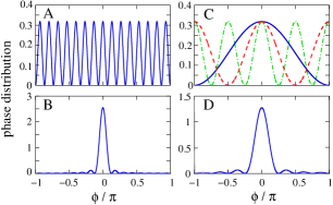
Figure 1: Phase probability distribution Eq.(6) with $p=1$, $N_{T}=15$ (A), and Eq.(9) with $p=4$, $N_{T}=15$ (B). In both cases, the total number of particles is the same, but the distribution of B gives a phase sensitivity at the Heisenberg limit. In C we plot the terms $\cos^{2}(2^{k}\phi/2)$ of Eq.(9). The solid blue line is for $k=0$, the dashed red line for $k=1$ and the dot-dashed green line for $k=2$. By multiplying these three distributions, as in Eq.(9), all peaks, except the one centered around the true value of the phase shift, $\theta=0$, are washed out to give the phase distribution D ($N_{T}=7$ and $p=3$).

Bayesian analysis with Schrödinger Cats. In the following, we discuss the Bayesian phase estimation strategy considering the Schrödinger cat states realized with trapped ions by Wineland and collaborators Leibfried_2003 ; Leibfried_2004 ; Leibfried_2005 . The state $|\Psi_{N}\rangle=(|N\downarrow\rangle+i^{\xi+N+1}|N\uparrow\rangle)/\sqrt{2}$ was created by applying the “nonlinear beam splitter” operator $\hat{U}_{N}=e^{i\frac{\pi\xi}{2}\hat{J}_{x}}e^{i\frac{\pi}{2}\hat{J}_{x}^{2}}$ to $N$ spin-down ions $|N\downarrow\rangle\equiv|\downarrow\rangle_{1}...|\downarrow\rangle_{N}$, with $\xi=0$ when $N$ is even, and $\xi=1$ when $N$ is odd Molmer_1998 . The $|\Psi_{N}\rangle$ state is then shifted in phase by an unknown quantity $\theta$ (which has to be determined) by applying the operator $e^{-i\theta\hat{J}_{z}}$. The final state, obtained after a further application of $\hat{U}_{N}$, is projected over $|N\uparrow\rangle$. Quantum Mechanics provides the probability to have $|N\uparrow\rangle$ at the output (which will be denoted as a “yes” result), given the unknown phase shift $\theta$ and the number of particles, $N$, of the cat state: $P(\mathrm{yes}|N,\theta)=|\langle\uparrow N|\hat{U}_{N}e^{-i\theta\hat{J}_{z}}\hat{U}_{N}|N\downarrow\rangle|^{2}=\cos^{2}\big{(}\frac{N\theta}{2}\big{)}$. Notice that this probability is identical to Eq.(4). The probability to obtain a “no” result is, obviously, $P(\mathrm{no}|N,\theta)=1-P(\mathrm{yes}|N,\theta)$. A single interferometric experiment consists of $p$ independent measurements. We collect a number $p_{y}$ of “yes” and $p_{n}=p-p_{y}$ of “no” results with probability $P_{p}(p_{y},p_{n}|N_{T},\theta)$, $N_{T}$ being the total number of particles used in the $p$ measurements. According to the Bayes theorem Pezze_2006 ; Helstrom , we have $P_{p}(\phi|N_{T},p_{y},p_{n})P(N_{T},p_{y},p_{n})=P_{p}(p_{y},p_{n}|N_{T},\phi)P(\phi)$, where $P(\phi)$ is fixed by the prior knowledge and $P(N_{T},p_{y},p_{n})$ provides the normalization of $P_{p}(\phi|N_{T},p_{y},p_{n})$, which is a phase probability distribution. We have

$$P_{p}(\phi|N_{T},p_{y},p_{n})\approx\prod_{j=1}^{p_{y}+p_{n}}P(\phi|N_{j},r_{j}),$$ (5)

where $N_{T}=\sum_{j=1}^{p_{y}+p_{n}}N_{j}$ and $r_{j}\equiv\mathrm{yes}$ ($\mathrm{no}$) if, in the $j-{\mathrm{th}}$ measurement, done with $N_{j}$ particles, we obtain a “yes” (“no”) result. Equation(5) contains all the available information needed to estimate $\theta$. We can choose, as estimator $\Theta_{est}$, the maximum of the phase distribution, and, as uncertainty $\Delta\Theta$, the $68\%$-confidence interval Pezze_2006 , namely the phase interval containing $68.27\%$ probability given by $\int_{\Theta_{est}-\Delta\Theta}^{\Theta_{est}+\Delta\Theta}\mathrm{d}\phi\,P_{p}(\phi|N_{T},p_{y},p_{n})=0.6827$. In the following, for analytical simplicity, we will consider, unless explicitly specified, the case in which the measurement results are only “yes”: $p_{y}=p$, $p_{n}=0$. That happens with certainty at $\theta=0$. The extension to an arbitrary value of $\theta$, where both “yes” and “no” are accessible, will be discussed in Pezze , also including decoherence effects.

$1/N_{T}$ periodicity of the Bayesian phase distribution. Let us first analyze the interferometric experiment with a state $|\Psi_{N_{T}}\rangle$ of $N_{T}$ particles and a single measurement: $p=1$. The phase distribution becomes

$$P_{1}(\phi|N_{T},p_{y}=1,p_{n}=0)\propto\cos^{2}(N_{T}\phi/2).$$ (6)

This probability contains $N_{T}$ peaks separated by a distance $2\pi/N_{T}$, see Fig.(1,A). Hence, our best guess about the real phase shift $\theta$ is $\Theta_{est}=\frac{2\pi}{N_{T}}n\pm\frac{\sqrt{2}}{N_{T}}$ with $n=0,1,\ldots,N_{T}-1$, where the error $\sqrt{2}/N_{T}$ is the mean square fluctuation around a single peak. In practice, we do not have any alternative but to choose, as phase estimator, one of the $N_{T}$ equivalent peaks of the distribution [cf. discussion after Eq.(4)]. In this case, however, the interferometric experiment does not give any substantial improvement in phase sensitivity. Tautologically, the phase uncertainty would scale with the total number of atoms as $\sim 1/N_{T}$ only if we have the a priori knowledge that the phase lies in an interval of width $2\pi/N_{T}$ around the real value. The $N_{T}$-peaks structure of Fig.(1,A) does not allow the Heisenberg limit, even in the case of arbitrary small incremental phase shifts. How is, therefore, possible to to select the “right” peak, so to speak, in order to build an unambiguous phase estimator?

The $\Delta\theta\sim N^{-3/4}$ limit. In this section we consider multiple independent measurements with different number of particles. The first measurement is done with a cat state of a single particle, $N=1$ (with a prior knowledge of the phase shift in the interval $[-\pi,\pi]$). We then perform a second measurement with $N=2$, and we multiply the resulting distribution with the previous one. We repeat this procedure $p$ times, increasing, in each shot, the number of particles in an arithmetic sequence $N=1,2,3,...,p$. The total number of particles is $N_{T}=p(p+1)/2$, and the phase distribution is

$$P_{p}\big{(}\phi|N_{T},p_{y}=p,p_{n}=0\big{)}\propto\prod_{k=1}^{p}\cos^{2}\bigg{(}\frac{k\phi}{2}\bigg{)}.$$ (7)

In the limit of large $p$, a Gaussian approximation gives $\prod_{k=1}^{p}\cos^{2}(k\phi)\approx\exp\big{[}-\frac{\phi^{2}}{4}\frac{p(p+1)(2p+1)}{6}\big{]}$, where $\sum_{k=1}^{p}k^{2}=p(p+1)(2p+1)/6$. For $p\gg 1$ we have $N_{T}\sim p^{2}/2$, and $\Delta\Theta=(9/2)^{1/4}/N^{3/4}_{T}$, which is in good agreement with the numerical calculation:

$$\Delta\Theta=\frac{1.44}{N^{3/4}_{T}}.$$ (8)

This argument can be generalized to the case of any prior phase knowledge $[-\pi/L,\pi/L]$, with $L\geq 1$. The goal is to obtain an unbiased estimate of $\theta$ within a region $2\pi/L$, the peaks outside this region being wiped out but the prior knowledge. As before, the protocol requires $p$ measurements: the first one with $\tilde{N}\approx L$ particles, the second one with $2\tilde{N}$, …, the last one with $p\tilde{N}$. The total number of particles is $\tilde{N}\,p\,(p+1)/2$. In the limit of large $p$, we obtain an unbiased phase estimate with a sensitivity $\Delta\Theta=\frac{1.44}{\tilde{N}^{1/4}}\frac{1}{N_{T}^{3/4}}$. With an arbitrary value of the true phase shift $\theta\neq 0$, the same protocol provides a distribution peaked about $\theta$ with a sensitivity scaling as $\sim 1/N_{T}^{3/4}$ for $N_{T}\gg 1$. This because the $\cos$ and $\sin$ distributions corresponding to “yes” and “no” results overlap out of phase and cancel out each other except in a region around $\theta$. Yet, even if the scaling $\sim 1/N_{T}^{3/4}$ overcomes the shot-noise Eq.(1), still this is not the fundamental limit.

The Heisenberg $\Delta\theta\sim N^{-1}$ limit. Let us now consider $p$ independent measurements done with a geometric sequence of particles, $N=1,2,4,8,...2^{p-1}$. The phase distribution becomes

$$P_{p}(\phi|N_{T},p_{y}=p,p_{n}=0)\propto\prod_{k=0}^{p-1}\cos^{2}\Big{(}\frac{2^{k}\phi}{2}\Big{)},$$ (9)

where the total number of particles employed in the complete process is $N_{T}=2^{p}-1$. Fig.(1,B) shows the case $p=4$, $N_{T}=15$, with a prior $-\pi\leq\theta\leq\pi$. Again, the width of the distribution can be simply calculated with a Gaussian approximation of each $\cos^{2}\big{(}\frac{2^{k}\phi}{2}\big{)}$ term, giving $P_{p}(\phi|N_{T},p_{y}=p,p_{n}=0)\simeq\exp[-\frac{\phi^{2}}{4}\frac{(2^{p}+1)(2^{p}-1)}{3}]$. In the limit of large $p$ we obtain a phase sensitivity at the Heisenberg limit $\Delta\Theta=\sqrt{6}/N_{T}$. The numerical calculation gives, asymptotically in the number of measurements $p$,

$$\Delta\Theta=\frac{2.55}{N_{T}}$$ (10)

for a $68\%$ confidence nota2 . We therefore conclude that it is possible to obtain an unbiased phase estimation at the Heisenberg limit, with repeated measurements and complete prior ignorance. The trick is to carefully choose the number of particles in each measurement and to multiply the corresponding phase probabilities so to cancel out the extra peaks of the phase distribution, see Figs.(1). To clarify this effect, let us consider a phase distribution obtained with $2^{k}$ particles: $\cos^{2}(2^{k}\phi/2)$. This has maxima in $\phi_{max}^{k}(n)=2\pi n/2^{k}$, with $n=0,\pm 1,...,\pm(2^{k}-1)$. Conversely, the phase distribution obtained with $2^{k-1}$ particles has minima in $\phi_{min}^{k-1}(n)=2\pi n/2^{k}$ with $n=\pm 1,\pm 3,...,\pm(2^{k-1}-1)$. By multiplying the two distributions, the maxima $\phi_{max}^{k}(n)$ superimpose with the minima $\phi_{min}^{k-1}(n)$, for $n=\pm 1,\pm 3,...$. When taking into account also the distributions with $2^{k-2},2^{k-3},...$ particles, we obtain the cancellation of all peaks $\phi_{max}^{k}(n)$ with $n=\pm 1,...,\pm(2^{k}-1)$ except the central one, $\phi_{max}^{k}(n=0)$, which is enhanced and has a width scaling as $\sim 1/2^{k}\sim 1/N_{T}$, see Figs.(1, C,D). This shows that the protocol employing $N=1,2,4,...,2^{p}$ particles is optimal and gives the Heisenberg limit with the best prefactor. Indeed, let us consider a general sequence $N=1,r,r^{2},...,r^{p-1}$, with an arbitrary integer $r$. If $r=1$, we recover the shot-noise limit Eq.(1), for $r=2$, we have, as already discussed, a perfect superposition of maxima and minima. For $r>2$, the phase distribution is characterized by several, strongly weighted, peaks which increase the phase uncertainty. To overcome this problem we must repeat $M>1$ times each interferometric measurement with a NOON state of fixed $N$ before increasing the number of particles (employing a total $N_{T}=M\sum_{k=0}^{p-1}r^{k}$). For a sufficient large $M$, it is possible to recover the Heisenberg limit Eq.(2), but at the price of a higher prefactor. In fact, we have that $\Delta\theta\sim\sqrt{M}/N_{T}$, as a consequence of the statistics of independent measurements. In Fig.(2) we analyzed the sensitivity obtained with different $r$ as a function of $M$: for $r=2$ (black circles) the best performance is obtained at $M=1$, for $r=3$ (blue points) at $M=4$, for $r=4$ (red diamonds) at $M=6$ and for $r=5$ (green squares) at $M=9$.

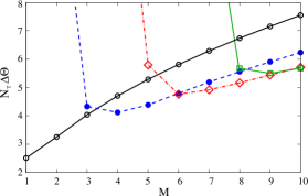
Figure 2: Phase sensitivity obtained with $N=1,r,r^{2},...,r^{p-1}$, where each measurement (using $N=r^{k}$ particles) is repeated $M$ times. The best strategy is obtained when $r=2$ (black circles) and $M=1$, due to a perfect superposition of maxima and minima in the Bayesian distributions, see Fig.(1,D). Notice that the optimal value of $M$, as well as the phase uncertainty, increases with $r$: here we consider $r=3$ (blue points), $r=4$ (red diamonds) and $r=5$ (green squares). Lines are guide to the eye.

As mentioned before, the analysis can be extended to estimate an arbitrary unknown phase shift $\theta\neq 0$. However, in contrast to the $\Delta\theta\sim N_{T}^{-3/4}$ case, here we have to consider multiple repeated measurements in order to concentrate the probability in a single peak, even for the case $r=2$. While the scaling $\sim 1/N_{T}$ is preserved Pezze , Eq.(10) gives a lower bound of phase sensitivity.

Sub shot-noise with Beryllium ions. The experimental demonstration of the Heisenberg limit would require the creation of Schrödinger cats having $N=8$ particles. The biggest Schrödinger cat created experimentally so far is with $N=6$ ${}^{9}\mathrm{Be}^{+}$ ions. This is still sufficiently large to reach a sub shot-noise phase sensitivity nota1 . In the following, we demonstrate, using the fidelities measured experimentally in Leibfried_2003 ; Leibfried_2004 ; Leibfried_2005 with Beryllium ions, the possibility to reach a phase sensitivity gain of 0.8 $db$ with respect to shot-noise for a priori $-\pi\leq\theta\leq\pi$. The protocol is quite similar to the one discussed above and requires Bayesian probabilities calculated with different number of ions combined with $M$ replica of the measurement process. We remark, however, that, in the analysis, we should now replace the ideal probability distributions with those retrieved experimentally. Indeed, we need to include the effects of noise and decoherence present in the experiments which will inevitably decrease the sensitivity of the interferometer. This step can be considered as a “calibration”: once the experimental probabilities are retrieved and inverted with Bayes, the interferometer is ready for its use. Many sources of experimental imperfections and decoherence conspire against phase uncertainty enhancement with cat states. Laser intensity fluctuations and magnetic field noise have been discussed in Leibfried_2005 . Imperfections in the creation of the state (3) due to non ideal $\hat{U}_{N}$ and decoherence have the common effect to decrease the oscillation amplitude of $P(\mathrm{yes}|N,\theta)$ Huelga_1997 .

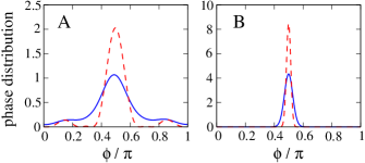
Figure 3: Phase probability distributions obtained by combining $M$ times (in (A) $M=1$, in (B) $M=10$) the Bayesian distributions for $N=1,\,2,\,3,\,4,\,5,\,6$ particles and $\theta=\pi/2$. The dashed red line is the ideal case, while the solid blue line has been obtained with the experimental fidelities, see exp_data .

A fit of the experimental probabilities with $P_{exp}(\mathrm{yes}|N,\theta)=A+C_{N\uparrow,N\downarrow}/2\cos(N\theta)$ and $P_{exp}(\mathrm{no}|N,\theta)=1-P_{exp}(\mathrm{yes}|N,\theta)$ has been given in Leibfried_2003 ; Leibfried_2004 ; Leibfried_2005 with the values of A and $C_{N\uparrow,N\downarrow}$ reported in exp_data . The main effect of the experimental noise is to decrease the fringes contrast $C_{N\uparrow,N\downarrow}$, which, in the ideal case, is equal to one. The experimental Bayesian phase probability distribution associated to a detection of a “yes” or “no” result, $P_{exp}(\phi|N,\{\mathrm{yes},\mathrm{no}\})$, is obtained inverting $P(\{\mathrm{yes},\mathrm{no}\}|N,\theta)$. We are now ready to simulate a realistic phase estimation experiment with Beryllium ions: i) A “yes” or “no” result is chosen with probability $P(\{\mathrm{yes},\mathrm{no}\}|N,\theta)$ with an unknown, but fixed, value of $\theta$ and for different number of ions, $N=1,~{}2,~{}3,~{}4,~{}5,~{}6$; ii) We repeat these measurements $M$ times; iii) We calculate the Bayesian distribution associated with each “yes”/“no” result and values of $N$; iv) We multiply all Bayesian distributions obtained in iii). This provides the final phase probability, from which we retrieve the estimated value of the phase shift and its confidence. The total number of particles used in this process is $N_{T}=N_{p}M$, with $N_{p}=\sum_{k=1}^{6}k=21$. Ideally, with $N=1,2,...,p$, the phase sensitivity would scale as

$$\Delta\Theta=\frac{(9/8)^{1/4}}{N_{p}^{3/4}M^{1/2}}=\frac{(9/8)^{1/4}}{N_{p}^{1/4}N_{T}^{1/2}},$$ (11)

where $N_{p}=p(p+1)/2$. In Fig.(3) we plot the theoretical and experimental phase probabilities for $M=1$ and $M=10$. Notice that the experimental distribution for $M=1$ is characterized by a large tail. This arises from the reduced fringe visibility and it would strongly dilute the confidence of the phase estimation. On the other hand, by multiplying the $M=10$ distributions, step ii), we strongly decrease the weight of the tail with respect to the central peak, see Fig.(3,B), at the price, of course, to increase the shot-noise. It is worth to emphasize, however, that, because of noise and decoherence, at the end of the day we could, in principle, get an experimental phase sensitivity even worse than the classical shot noise. Asymptotically in $M$, the phase probability Eq.(5) can be written as

$$P_{exp}(\phi|N_{T},\theta) = \prod_{N=1}^{6}P_{exp}(\phi|N,\mathrm{yes})^{MP_{exp}(\mathrm{yes}|N,\theta)}\times$$ (12)

$$\times P_{exp}(\phi|N,\mathrm{no})^{MP_{exp}(\mathrm{no}|N,\theta)}.$$

In this limit, and with ideal fidelities, we would have a phase independent gain $G_{th}=3.18$ $db$ with respect to the shot-noise limit $\Delta\Theta_{sn}$. Such a gain would be comparable with the best performances obtained to date with photons McKanzie_2002 . As a consequence of imperfections and decoherence, the experimental gain is lower than the ideal prediction and depends on the phase shift, see the solid red line in Fig.(4). The maximum gain is $G_{exp}=0.75$ $dB$, around the optimal working point $\theta\sim 0.3$. In principle, an even higher gain can be obtained using states with $N=1,2,4,8,...,2^{p-1}$ particles: the sensitivity would be bounded by the ideal value

$$\Delta\Theta=\frac{2.55}{N_{p}M^{1/2}}=\frac{2.55}{N_{p}^{1/2}N_{T}^{1/2}},$$ (13)

with $N_{p}=2^{p}-1$.

So far we have considered the case of complete prior ignorance. While this can be important for technological and basic science applications like in gyroscopes or clock synchronizations, it is sometimes possible to confine the priori within an interval $-\pi/L\leq\theta\leq\pi/L$, with $L>1$. In this case an unbiased phase estimation can be obtained with $M$ replica of the interferometric measurement, each with a Schrödinger cat state of a fixed number of particles $\tilde{N}\simeq L$. With ideal distributions, we would obtain a phase-independent sensitivity $\Delta\Theta=\frac{1}{\tilde{N}^{1/2}\sqrt{N_{T}}}$, with $N_{T}=M~{}\tilde{N}$. The gain with respect to the shot-noise, obtained with the experimental probabilities, is shown in Fig.(4) where the arrows indicate the prior knowledge $\pi/\tilde{N}$ for the various cases.

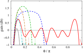
Figure 4: Gain (db) with respect to the shot-noise limit obtained with the experimental parameters exp_data . The blue dashed line is the case $N=2$, the green dot-dashed line $N=3$, the brown dot-dot-dashed line $N=4$, the sky-blue dot-dot-dot-dashed line $N=5$, and the black dotted line $N=6$. Colored arrows indicate the upper bound to the phase prior for each data set. With maximum priori ignorance, we combine $M$ replica of the Bayesian phase distributions with $N=1,2,3,4,5,6$, Eq.(12), (solid red line). The horizontal dotted line gives the shot-noise.

The gain is maximum at $\theta=\pi/(2\tilde{N})$ where the experimental probabilities to have a “yes” or “no” result are closer to the ideal ones. Notice that the sensitivity at first increases and eventually decreases with the number of ions. This is caused by the competition between the gain obtained increasing $\tilde{N}$ and the loss of visibility due to decoherence, which is higher for larger cats. With the experimental fidelities measured so far, the best scenario is obtained employing cat states of $\tilde{N}=3$ particles, which provides a gain up to $1.63$ $db$ with respect to the shot-noise. Yet, it is clear that, with a priori $-\pi/L\leq\theta\leq\pi/L$ and with cat states having a number of particles $\tilde{N}\simeq 2^{k}L$, with $k=1,2,3,...$, we can, in principle, further decrease the phase uncertainty than using cats with a fixed number of particles.

We remark that the total number of particles used in our phase estimation protocol can be arbitrarily large (being proportional to the number of replica $M$). This is important for realistic technological applications since the number of particles in Schrödinger cat states would probably remain relatively small, at least in the next future. We can expect to have, in a few years, the production of robust high-fidelity cat states up to $\sim 10$ photons or ions, allowing the saturation, at least in principle, of Eq.(2). Major obstacles to these efforts are creation imperfections and decoherence Huelga_1997 ; zurek . On the other hand, Bose Einstein Condensation might offer the possibility to create NOON states with a larger number of particles Dunningham_2001 . A different, promising strategy to experimentally reach sub shot-noise sensitivities is to use number-squeezed states, which have been recently experimentally demonstrated Orzel_2001 ; Chuu_2005 with up to few hundred neutral atoms. In any case, crucial to the success Heisenberg limited interferometry, is the realization of highly efficient number counting detectors, which can be probably developed in the next generation of experiments Chuu_2005 ; Khoury_2006 .

Conclusions. Ultra-sensitive interferometry requires unbiased phase estimation protocols and carefully engineered maximal quantum correlations among input states. In this paper we have developed a novel Bayesian protocol based on multiple measurements with Schrödinger cat states of variable number of particles. This achieves the Heisenberg sensitivity $\Delta\Theta\sim N_{T}^{-1}$ with an arbitrary prior phase uncertainty. This protocol overcomes difficulties present in previous approaches where the estimate was strongly ambiguous, so to require a prior knowledge of the true value of the phase in the restricted interval $-\pi/N_{T}\leq\theta\leq\pi/N_{T}$. We have also demonstrated the possibility to obtain sub shot-noise phase sensitivity with the experimental data published in Leibfried_2003 ; Leibfried_2004 ; Leibfried_2005 on the creation of Beryllium ions Schrödinger cat states. Our results do not depend on how the state Eq.(3) is created, nor on the specific interferometric apparatus as far as the phase probability distributions have an oscillating pattern with a period depending on the number of particles.

- (1) Giovanetti V., Lloyd S. and Maccone L. Phys. Rev. Lett. 96, 010401 (2006).
- (2) Pezzé L., Smerzi A., Khoury G., Hodelin J.F. and Bouwmeester D., quant-ph/0701158.
- (3) In this Letter we consider non interacting particles for which Eq.(2) represents the ultimate limit Giovannetti_2006 . Eq.(2) can be overcome with interacting particles, Luis A. Phys. Lett. A 329, 8 (2004); Roy S.M. and Braunstein S.L., quant-ph/0607152; Boixo S., Flammia S.T., Caves C.M. Geremia J.M. Phys. Rev. Lett. 98, 090401 (2007).
- (4) Caves C.M., Phys. Rev. D 23, 1693 (1981).
- (5) Yurke B., McCall S.L. and Klauder J.R., Phys. Rev. A 33, 4033 (1986); Holland M.J. and Burnett K., Phys. Rev. Lett. 71, 1355 (1993).
- (6) Pezzé L. and Smerzi A., Phys. Rev. A 73, 011801(R) (2006).
- (7) In this context, NOON states first appeared in Sanders B.C., Phys. Rev. A. 40, 2417 (1989), and they were independently introduced in Boto A.N., Kok P., Abrams D.S., Braunstein S.L., Williams C.P. and Dowling J.P. Phys. Rev. Lett. 63, 063407 (2001). The name “NOON” appeared in a footnote of Lee H., Kok P., Dowling J.P., J. Mod. Opt. 49, 2325 (2002).
- (8) Lamas-Linares A., Howell J.C. and Bouwmeester D., Nature 412, 887 (2001); Walther P., Pan J., Aspelmeyer M., Ursin R., Gasparoni S. and Zeilinger A., Nature 429, 158 (2004); Mitchell W.M., Lundeen J.S. and Steinberg A.M., Nature 429, 161 (2004).
- (9) Zhao A., Chen Y., Zhang A., Yang T., Briegel H.J. and Pan J., Nature 430, 54 (2004).
- (10) Leibfried D., DeMarco B., Mayes V., Lucas D., Barrett M.D., Britton J., Itano W.M., Jelenkovic B., Langer C., Rosenband T. and Wineland D.J., Nature 422, 412 (2003).
- (11) Leibfried D., Barrett M.D., Schaetz T., Britton J., Chiaverini J., Itano W.M., Jost J.D., Langer C. and Wineland D.J., Science 304, 1476 (2004).
- (12) Leibfried D., Knill E., Seidelin S., Britton J., Blakestad R.B., Chiaverini J., Hume D.B., Itano W.M., Jost J.D., Langer C., Ozeri R., Reichle R. and Wineland D.J., Nature 438, 639 (2005).
- (13) Giovanetti V., Lloyd S. and Maccone L., Science 306, 1330 (2004).
- (14) Bollinger J.J., Itano W.M., Wineland D.J. and Heinzen D.J., Phys. Rev. A 54, R4649 (1996); Gerry C.C. and Campos R.A., Phys. Rev. A 68, 025602 (2003).
- (15) Notice that, with a prior , the error propagation formula predicts a sensitivity Bollinger_1996 .
- (16) Rudolph T. and Grover L., Phys. Rev. Lett. 91, 217905 (2003).
- (17) Giovanetti V., Lloyd S. and Maccone L., Science 306, 417 (2001).
- (18) Mølmer K. and Sørensen A., Phys. Rev. Lett. 82, 1835 (1998).
- (19) Zawisky M., Hasegawa Y., Rauch H., Hradil Z., Myska R. and Perina J., J. Phys. A: Mat. Gen. 31, 551 (1998); Helstrom C.W., Quantum Detection and Estimation Theory Academic Press, New York (1976), cap.1.
- (20) Pezzé L. and Smerzi A., unpublished.
- (21) We have for a confidence and for a confidence.
- (22) With two ions, a phase sensitivity has been experimentally demonstrated in Meyer_2000 using an error propagation analysis and prior knowledge .
- (23) Meyer V., Rowe M.A., Kielpinski D., Sackett C.A., Itano W.M., Monroe C. and Wineland D.J., Phys. Rev. Lett. 86, 5870 (2001).
- (24) Huelga S.F., Macchiavello C., Pellizzari T., Ekert A.K., Plenio M.B. and Cirac J.I., Phys. Rev. Lett. 79, 3865 (1997).
- (25) The experimental parameters are , , Leibfried_2003 , Leibfried_2004 , , and Leibfried_2005 .
- (26) McKanzie K., Shaddock D.A., McClelland D.E., Butchler B.C. and Lam P.K. Phys. Rev. Lett. 88, 231102 (2002); and ref.s therein.
- (27) Zurek W.H., Rev. Mod. Phys. 75, 715 (2003); André A., Sørensen A.S. and Lukin M.D., Phys. Rev. Lett. 92, 230801 (2004).
- (28) Dunningham J.A. and Burnett K., J. Mod. Opt. 48, 1837 (2001); Sørensen A, Duan L.M., Cirac J.I. and Zoller P., Nature 409, 63 (2001).
- (29) Orzel C., Tuchman A.K., Fenselau M.L., Yasuda M. and Kasevich M.A., Science 291, 2386 (2001); Greiner M., Madel O., Esslinger T., Hänsch T.W. and Bloch I., Nature 415, 39 (2002); Jo G.B., Shin Y., Will S., Pasquini T.A., Saba M., Ketterle W., Pritchard D.E., Vengalattore M. and Prentiss M., Phys. Rev. Lett. 98, 030407 (2007); Li W., Tuchman A.K., Chien H. and Kasevich M.A., Phys. Rev. Lett. 98, 040402 (2007).
- (30) Chuu C.S., Schreck F., Meyrath T.P., Hanssen J.L., Price G.N. and Reizen M.G., Phys. Rev. Lett. 95, 260403 (2005).
- (31) Khoury G., Eisenberg H.S., Fonseca E.J.S., and Bouwmeester D., Phys. Rev. Lett. 96, 203601 (2006).