An “anti-Gleason” phenomenon and simultaneous measurements in classical mechanics

Abstract

We report on an “anti-Gleason” phenomenon in classical mechanics: in contrast with the quantum case, the algebra of classical observables can carry a non-linear quasi-state, a monotone functional which is linear on all subspaces generated by Poisson-commutative functions. We present an example of such a quasi-state in the case when the phase space is the 2-sphere. This example lies in the intersection of two seemingly remote mathematical theories – symplectic topology and the theory of topological quasi-states. We use this quasi-state to estimate the error of the simultaneous measurement of non-commuting Hamiltonians.

1 Introduction

Let ${\mathcal{A}}_{q}$ (resp. ${\mathcal{A}}_{c}$) be the algebra of observables in quantum (resp. classical) mechanics. In the quantum case, ${\mathcal{A}}_{q}$ is the space of hermitian operators on a Hilbert space $H$. It is equipped with the bracket $[A,B]_{\hbar}=\frac{i}{\hbar}(AB-BA)\,,$ where $\hbar$ is the Planck constant. In the classical case, ${\mathcal{A}}_{c}$ is the space of continuous real-valued functions on a symplectic manifold $(M,\omega)$. It is equipped with the Poisson bracket $\{\cdot,\cdot\}$ (defined on a dense subspace of smooth functions). We say that observables $A$ and $B$ commute if their bracket vanishes.

In [23] von Neumann introduced the notion of a quantum state. According to his definition, a state is a functional $\rho:{\mathcal{A}}_{q}\to{\mathbb{R}}$ which satisfies:

(Linearity) $\rho(aA+bB)=a\rho(A)+b\rho(B)$ for all $a,b\in{\mathbb{R}}$ and all $A,B\in{\mathcal{A}}_{q}$;

(Positivity) $\rho(A)\geq 0$ provided $A\geq 0$;

(Normalization) $\rho(1)=1$.

This system of axioms implies that for every quantum state $\rho$ there exists a density operator $U$, that is a nonnegative Hermitian operator on $H$ having trace $1$, so that $\rho(A)=\operatorname{tr}(UA)$ for every observable $A\in{\mathcal{A}}_{q}$.

Von Neumann’s notion of quantum state encountered criticism among physicists (for example, see [4]) in that the formula $\rho(A+B)=\rho(A)+\rho(B)$ a priori makes sense only if the observables $A$ and $B$ are simultaneously measurable, which in the mathematical language means that they commute. As a response to the criticism there appeared the concept of a quasi-state. A quasi-state on ${\mathcal{A}}$ (here ${\mathcal{A}}$ stands either for ${\mathcal{A}}_{q}$ or ${\mathcal{A}}_{c}$) is a functional $\zeta:{\mathcal{A}}\to{\mathbb{R}}$ satisfying the positivity and normalization axioms above, and a weaker form of linearity, the so-called

(Quasi-linearity) $\zeta(aA+bB)=a\zeta(A)+b\zeta(B)$ for all $a,b\in{\mathbb{R}}$ and all commuting observables $A,B\in{\mathcal{A}}$.

A remarkable fact, which is a straightforward reformulation of the famous theorem due to Gleason [13], is as follows:

Theorem 1.1 (Gleason).

On a Hilbert space of dimension at least $3$, every quasi-state is linear.

Therefore in the quantum case there is no distinction between states and quasi-states.

Some brief comments on the Gleason theorem are in order. The key notion responsible for Gleason’s phenomenon and which is of an independent significance in the subject of quantum logic is a probability measure on projections: Let ${\mathcal{P}}$ be the set of orthogonal projection operators on $H$, that is the simplest observables which attain values $1$ and $0$ only. They can be interpreted as yes-no experiments. Call two such operators $P,Q\in{\mathcal{P}}$ orthogonal to one another, if their ranges are orthogonal as subspaces of $H$. Note that orthogonal projections commute. Given a collection $\{P_{i}\}$ of pairwise orthogonal projections, their sum $\sum_{i}P_{i}$ is again an orthogonal projection. A probability measure on projections is a function $\mu:{\mathcal{P}}\to[0,1]$ with $\mu(1)=1$ satisfying the following $\sigma$-additivity property (cf. [16, p.132]): $\mu\big{(}\sum_{i}P_{i}\big{)}=\sum_{i}\mu(P_{i})$ for any collection $\{P_{i}\}$ of pairwise orthogonal projection operators. By an ingenious argument Gleason shows that for every such $\mu$ there exists a density operator $U$ so that $\mu(P)=\operatorname{tr}(UP)$ for all $P\in{\mathcal{P}}$. Given any quasi-state $\zeta$, its restriction to ${\mathcal{P}}$ is a probability measure on projections, and hence $\zeta(P)=\operatorname{tr}(UP)$ for some density operator $U$. In view of the spectral decomposition, every Hermitian operator $A\in{\mathcal{A}}_{q}$ can be written as a real linear combination of pairwise orthogonal projections. Thus quasi-linearity of $\zeta$ yields $\zeta(A)=\operatorname{tr}(UA)$, and in particular $\zeta$ is linear.

The Gleason theorem plays an important role in quantum mechanics. It provides a counter-argument to the above-mentioned criticism of von Neumann’s concept of quantum state, and thus validates representation of states by density operators which serve as a cornerstone for probabilistic formalism in quantum mechanics. Furthermore, the Gleason theorem stimulated a number of exciting developments related to the hidden variables problem. For instance, a starting point for the seminal works by Bell [4] and Kochen-Specker [17] is the following observation: Existence of non-contextual hidden variables would yield existence of dispersion-free states and hence supply the quantum theory with the possibility of an assignment of a definite outcome to every yes-no experiment. Such an assignment would be nothing else but a probability measure on projections attaining values $0$ and $1$ only. One readily sees that this is prohibited by the Gleason theorem.

The purpose of this note is to show that in classical mechanics the situation is quite different. In fact, we report on the following ”anti-Gleason phenomenon”: for certain symplectic manifolds, the algebra of classical observables ${\mathcal{A}}_{c}$ carries non-linear quasi-states. Since algebras of classical observables often arise as a limit of algebras of quantum observables as $\hbar\to 0$, our result can be interpreted as the failure of the Gleason theorem in the classical limit. In Section 2 we describe the simplest meaningful example of a non-linear quasi-state in the case when the underlying symplectic manifold is the $2$-sphere equipped with an area form. Such a phase space appears for instance as the classical limit of the high spin quantum particle, see Section 4. As an application of our quasi-state, we indicate in Section 3 that it gives rise to a robust lower bound for the error of a simultaneous measurement (in a sense to be made precise) of a pair of non-commuting classical observables.

Complete formulations and proofs of the results discussed below can be found in our papers [10, 11, 12].

2 A non-linear quasi-state on ${\mathbb{S}}^{2}$

Consider the unit $2$-sphere ${\mathbb{S}}^{2}\subset{\mathbb{R}}^{3}(x,y,z)$. Let $\omega$ be the area form induced from the Euclidean metric and divided by $4\pi$, so that the total area of the sphere equals $1$.

Let $F$ be a generic function on ${\mathbb{S}}^{2}$. Consider its Reeb graph $\Gamma_{F}$ obtained from the sphere by collapsing each connected component of each level set $\{F=\text{const}\}$ to a point. This notion was first considered by Reeb [22] in the framework of Morse theory (see e.g. [9] for a detailed discussion). It is illustrated on Figs. 2, 2. Since it is hard to visualize a complicated function on the round sphere ${\mathbb{S}}^{2}$, we employ the following trick: we represent the sphere as a surface in ${\mathbb{R}}^{3}$ (possibly of complicated shape), and take $F$ to be the height function $F(x,y,z)=z$ on it. It can be easily seen that $\Gamma_{F}$ is a tree. For a point $a\in\Gamma_{F}$ denote by $C(a)$ the corresponding connected component of the level set. If $a$ is a vertex of the graph, $C(a)$ is either a point of local extremum, or a “figure eight” with the double point at a saddle. If $a$ is an interior point of an edge, $C(a)$ is a simple closed curve on the sphere.

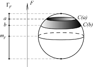
Figure 1: Round sphere. The Reeb graph $\Gamma_{F}$ is a segment.

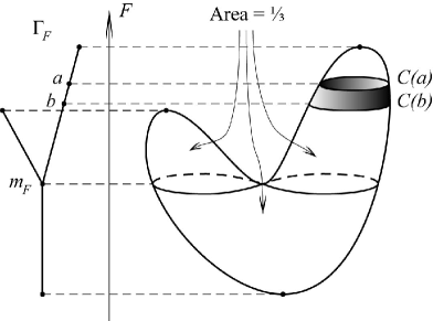
Figure 2: Deformed sphere. The Reeb graph $\Gamma_{F}$ is a tripod.

Introduce a probability measure $\sigma$ on $\Gamma_{F}$ in the following way. Consider any open interval $I=(a,b)$ on an edge of $\Gamma_{F}$. It corresponds to the annulus on ${\mathbb{S}}^{2}$ bounded by curves $C(a)$ and $C(b)$ (see Figs. 2, 2). By definition, the measure $\sigma(I)$ of the interval $I$ is equal to the area of this annulus.

Given such a tree $\Gamma_{F}$ with the probability measure $\sigma$, there exists a unique point $m_{F}$ on it, called the median of the tree, with the following property: when $m_{F}$ is removed from $\Gamma_{F}$, the resulting set breaks up into connected components, each of measure $\leq\frac{1}{2}$ – see Figs. 2, 2; on Fig. 2 the median is the midpoint of the segment $\Gamma_{F}$; on Fig. 2 the median is the triple point of the tripod. Define $\zeta(F)$ as the value of $F$ on the level $C(m_{F})$.

For example, if $F(x,y,z)=x$ (on the round ${\mathbb{S}}^{2}$), the tree $\Gamma_{F}$ is simply the segment $[-1;1]$, its median $m_{F}$ is the point $0$, and the level $C(m_{F})$ coincides with the equator $\{x=0\}$. Hence

$$\zeta(x)=0\;.$$ (1)

We claim that $\zeta(F)\leq\zeta(G)$ for any pair of generic functions $F$ and $G$ with $F\leq G$. Indeed, each connected component of the sets ${\mathbb{S}}^{2}\setminus C(m_{F})$ and ${\mathbb{S}}^{2}\setminus C(m_{G})$ is a disc of area $\leq\frac{1}{2}$. Therefore $C(m_{F})$ and $C(m_{G})$ must intersect at some point, say, $P$. Then

$$\zeta(F)=F(P)\leq G(P)=\zeta(G)$$

and the claim follows.

Write $\|F\|$ for the uniform norm $\max_{{\mathbb{S}}^{2}}|F|$. The monotonicity property above yields that

$$|\zeta(F)-\zeta(G)|\leq\|F-G\|$$

for all generic functions $F$ and $G$. Thus we can extend $\zeta$ by continuity to the whole space ${\mathcal{A}}_{c}$.

It turns out that $\zeta:{\mathcal{A}}_{c}\to{\mathbb{R}}$ is a quasi-state. Obviously, it satisfies the normalization and the positivity axioms. Let us illustrate the quasi-linearity axiom. For simplicity, we verify the property

$$\{F,G\}=0\Rightarrow\zeta(F+G)=\zeta(F)+\zeta(G)$$

in the case when the functions $F,G$ and $F+G$ are generic. Note that in this case the assumption $\{F,G\}=0$ simply means that $F,G$ and $F+G$ are pairwise functionally dependent and therefore have the same connected components of the level sets. One can easily conclude that the curves $C(m_{F}),C(m_{G})$ and $C(m_{F+G})$ coincide. Denoting this curve by $C$ we have that for every point $P\in C$

$$\zeta(F+G)=(F+G)(P)=F(P)+G(P)=\zeta(F)+\zeta(G)\;,$$

as required.

We shall refer to the quasi-state $\zeta$ as the median quasi-state.

Assume that $F:{\mathbb{S}}^{2}\to{\mathbb{R}}$ is a generic function. For a continuous function $u:{\mathbb{R}}\to{\mathbb{R}}$ consider the composition $G(x,y,z)=u(F(x,y,z))$, which can be already non-generic. It is not hard to show that

$$\zeta(G)=u(\zeta(F))\;.$$ (2)

We shall apply this formula in order to calculate $\zeta(G)$, where $G(x,y,z)=x^{2}$. Note that $G$ has a circle of minima points and hence is not generic. Put $F(x,y,z)=x$ and $u(s)=s^{2}$ so that $G(x,y,z)=u(F(x,y,z))$. Combining formulas (2) and (1) we get that $\zeta(x^{2})=\zeta(x)^{2}=0$. Similarly, $\zeta(y^{2})=\zeta(z^{2})=0$.

Finally, let us verify that the median quasi-state is non-linear. Indeed, since on ${\mathbb{S}}^{2}$ we have $x^{2}+y^{2}+z^{2}=1$, it follows from the definition of a quasi-state that $\zeta(x^{2}+y^{2})=1-\zeta(z^{2})=1$. Thus

$$\zeta(x^{2}+y^{2})-\zeta(x^{2})-\zeta(y^{2})=1\;.$$ (3)

3 Simultaneous classical measurements

Two non-commuting quantum observables are not simultaneously measurable. Is there an analogous phenomenon in classical mechanics? This problem appears in physics literature (see e.g. books by Peres [21, Chapter 12-2] and Holland [14, Chapter 8.1]) as a toy example motivating the theory of quantum measurements. Theoretically, in a classical system any two observables are simultaneously measurable to any accuracy. However, if the measurement is not perfect, an error may appear. Below we present a precise formulation of these heuristic notions and give a positive answer to the above question.

We shall analyze simultaneous measurability in classical mechanics in the framework of a measurement procedure called the pointer model. For simplicity we work on the sphere ${\mathbb{S}}^{2}$ and write $\zeta$ for the median quasi-state introduced in the previous section. We denote by $\|F\|$ the uniform norm of a function $F$ on ${\mathbb{S}}^{2}$ and by $\langle F\rangle$ its mean value $\int_{{\mathbb{S}}^{2}}F\cdot\omega$. For a pair of smooth functions $F_{1},F_{2}$ on the sphere consider the quantity

$$\Pi(F_{1},F_{2})=|\zeta(F_{1}+F_{2})-\zeta(F_{1})-\zeta(F_{2})|$$

which measures the non-additivity of $\zeta$ at this pair. Define also the oscillation

$$\operatorname{osc}(F_{1},F_{2})=\min\big{(}\|F_{1}-\langle F_{1}\rangle\|,\|F_{2}-\langle F_{2}\rangle\|\big{)}\;.$$

Consider two observables $F_{1},F_{2}\in{\mathcal{A}}_{c}$. Let $M={\mathbb{S}}^{2}\times{\mathbb{R}}^{4}(p_{1},q_{1},p_{2},q_{2})$ be the extended phase space equipped with the symplectic form $\widehat{\omega}=\omega+dp_{1}\wedge dq_{1}+dp_{2}\wedge dq_{2}$ . The ${\mathbb{R}}^{4}$ factor corresponds to the measuring apparatus (the pointer), whereas $\vec{q}=(q_{1},q_{2})$ is the quantity read from it. The coupling of the apparatus to the system is carried out by means of the Hamiltonian function $p_{1}F_{1}(v)+p_{2}F_{2}(v)$, $v\in{\mathbb{S}}^{2}$. The Hamiltonian equations of motion with the initial conditions $q_{1}(0)=q_{2}(0)=0,p_{1}(0)=p_{2}(0)=\epsilon$ and $v(0)=w$ are as follows:

$$\dot{q_{i}} =F_{i},\;i=1,2,$$

$$\dot{p_{i}} =0,\;i=1,2,$$

$$\dot{v} =\epsilon\ V_{F_{1}+F_{2}}(v)\;.$$

Here $V_{F_{1}+F_{2}}$ denotes the Hamiltonian vector field of the Hamiltonian $F_{1}+F_{2}$ on ${\mathbb{S}}^{2}$.

Denote by $g_{t}$ the Hamiltonian flow on ${\mathbb{S}}^{2}$ generated by the function $G=F_{1}+F_{2}$. Then $v(t)=g_{\epsilon t}w$. Let $T>0$ be the duration of the measurement. By definition, the output of the measurement procedure is a pair of functions $F^{\prime}_{i},\;i=1,2,$ on $M$ defined by the average displacement of the $q_{i}$-coordinate of the pointer:

$$F^{\prime}_{i}(w)=\frac{1}{T}(q_{i}(T)-q_{i}(0))=\frac{1}{T}\int_{0}^{T}F_{i}(v(t))dt=\frac{1}{T}\int_{0}^{T}F_{i}(g_{\epsilon t}w)dt\;.$$

Note that for $\epsilon=0$ we have $F^{\prime}_{i}=F_{i}$. This justifies the above procedure as a measurement of $F_{i}$ and allows us to interpret the number $\epsilon$ as an imprecision of the pointer.

Define the error of the measurement as

$$\Delta(T,\epsilon,F_{1},F_{2})=\left\|F^{\prime}_{i}-F_{i}\right\|.$$

Note that in our setting this quantity does not depend on $i\in\{1;2\}$ since the sum $F_{1}+F_{2}$ is constant along the trajectories of $g_{t}$.

Now we are ready to formulate our main result [12]: for all $T,\epsilon>0$ and $F_{1},F_{2}\in{\mathcal{A}}_{c}$

$$\Delta(T,\epsilon,F_{1},F_{2})\geq\frac{1}{2}\Pi(F_{1},F_{2})-\sqrt{\frac{2\cdot\operatorname{osc}(F_{1},F_{2})}{T\epsilon}}\;.$$ (4)

For $\epsilon>0$ define the asymptotic (as $T\to\infty$) error of the measurement as

$$\Delta_{\infty}(F_{1},F_{2})=\liminf_{T\to\infty}\Delta(T,\epsilon,F_{1},F_{2})\;.$$

It may be interpreted as the error produced in a system moving very rapidly, that is such that its characteristic time is much less than that of a measurement. Note that $\Delta(T,\epsilon,F_{1},F_{2})=\Delta(\epsilon T,1,F_{1},F_{2})$ and hence $\Delta_{\infty}$ does not depend on the specific choice of $\epsilon>0$. It follows from inequality (4) that

$$\Delta_{\infty}(F_{1},F_{2})\geq\frac{1}{2}\Pi(F_{1},F_{2})\;.$$ (5)

Define a numerical constant

$$E:=\inf_{F_{1},F_{2}}\frac{2\Delta_{\infty}(F_{1},F_{2})}{\Pi(F_{1},F_{2})}\;,$$

where the infimum is taken over all pairs of smooth observables $F_{1}$ and $F_{2}$ on the sphere with $\Pi(F_{1},F_{2})\neq 0$. Note that $E\geq 1$ in view of $\eqref{eq-asymp}$. To find an upper bound on $E$, consider the case $F_{1}=x^{2}$ and $F_{2}=y^{2}$. An elementary but cumbersome calculation shows that $\Delta_{\infty}(x^{2},y^{2})\sim 0.63$. Equation (3) above yields $\Pi(x^{2},y^{2})=1$. Therefore $E\leq 1.26$. It would be interesting to calculate the value of $E$ explicitly.

Let us emphasize a somewhat surprising feature of inequality (4). Its right-hand side is robust with respect to small perturbations of both observables in the uniform norm. On the other hand, the measurement error $\Delta$ involves the Hamiltonian flow generated by $F_{1}+F_{2}$ which is defined by the first derivatives of $F_{1}$ and $F_{2}$. Therefore a priori $\Delta(T,\epsilon,F_{1},F_{2})$ could have changed in an arbitrary way after such a perturbation, in particular it could have vanished, but this does not happen provided $\Pi(F_{1},F_{2})\neq 0$.

It is instructive to mention that our lower bound (4) on the error of the simultaneous measurement of a pair of classical non-commuting observables $F_{1},F_{2}$ with $\Pi(F_{1},F_{2})\neq 0$ cannot be considered as a classical version of the uncertainty principle. Indeed, the quantum uncertainty principle deals with the statistical dispersion of similarly prepared systems [3, p.379]. Let us interpret for a moment the quantity $\zeta(F)$ as the statistical expectation of the value of the observable $F$ in the (quasi-)state $\zeta$. With this language, the quasi-state $\zeta$ introduced in Section 2 is dispersion free: $\zeta(F^{2})-\zeta(F)^{2}=0$ for all $F$ (see [11]).

4 Discussion: the classical limit of quantum spin system

It is an intriguing question [15] to understand “what went wrong” with the proof of the Gleason theorem in the classical context. Our impression is that the notion of the probability measures on projections, which is the key character of the proof (see Section 1 above), does not admit a natural translation into the classical language via the quantum-classical correspondence. However, instead of considering the “anti-Gleason” phenomenon as a failure of the correspondence principle, we propose to address the above question the other way around:

Question 4.1.

Is there a footprint of the median quasi-state $\zeta$ in the quantum world?

To be more specific, recall that the algebra of functions on the 2-sphere ${\mathbb{S}}^{2}$ equipped with the Poisson bracket arises as the classical limit of a quantum spin system. Below we briefly review a construction called the coherent states (de)quantization [6, 20]. Consider a quantum particle of spin $j$ where $j>0$ is an integer or a half integer number. The quantum states are modeled by vectors of a Hilbert space $H$ of dimension $N=2j+1$ which carries an irreducible representation of the group $SU(2)$. Denote by $K:=S^{1}\subset SU(2)$ the subgroup consisting of diagonal matrices. A standard argument of the representation theory yields the existence of a $K$-invariant complex line $\ell\subset H$ such that $K$ acts on $\ell$ as the full $2j$-turn rotation. Fix a unit vector $|\psi\rangle\in\ell$.

Denote by ${\mathcal{M}}(N)$ the algebra of complex linear operators of $H$. Given an operator $A\in{\mathcal{M}}(N)$, define a function $\hat{s}_{A}:SU(2)\to{\mathbb{C}}$ by $\hat{s}_{A}(g)=\langle g\psi|Ag\psi\rangle$. A crucial observation is as follows: given $k\in K$, we have $k|\psi\rangle=e^{i\theta}|\psi\rangle$ for some $\theta\in{\mathbb{R}}$, and therefore $\hat{s}_{A}(gk)=\hat{s}_{A}(g)$ for all $g\in SU(2),k\in K$. This means that $\hat{s}_{A}$ descends to a smooth function, say $s_{A}$, on the quotient space $SU(2)/K$. This quotient space is naturally identified with the 2-sphere ${\mathbb{S}}^{2}$. The function $s_{A}$ on ${\mathbb{S}}^{2}$ is called the covariant symbol of the operator $A$. Note that the correspondence

$${\mathcal{M}}(N)\to C^{\infty}({\mathbb{S}}^{2}),\;A\mapsto s_{A}$$

sends the space of Hermitian operators ${\mathcal{A}}_{q}(N)\subset{\mathcal{M}}(N)$ to the space ${\mathcal{A}}_{c}$ of real-valued functions, and non-negative operators to non-negative functions.

Given any smooth function $a$ on ${\mathbb{S}}^{2}$, there exists a sequence of operators $A(N)\in{\mathcal{M}}(N)$ so that the corresponding covariant symbols $s_{A(N)}$ converge to $a$ as $N\to\infty$. Suppose now that $s_{A(N)}\to a$ and $s_{B(N)}\to b$ for a pair of functions $a,b$ on ${\mathbb{S}}^{2}$. It turns out that the following correspondence principle holds true:

$$s_{A_{N}B_{N}}\to ab,\;\;\text{and}\;\;N\cdot s_{[A(N),B(N)]}\to i\{a,b\}\;\;\text{as}\;\;N\to\infty.$$

This can be interpreted as follows: the algebra of classical observables ${\mathcal{A}}_{c}$ on the 2-sphere ${\mathbb{S}}^{2}$ equipped with the Poisson bracket arises as the high spin limit $N\to\infty$ of algebras ${\mathcal{A}}_{q}(N)$ of quantum observables. Let us also mention that a related construction of the fuzzy sphere [18] paved a road for extension of geometric analysis on the classical phase space into the framework of matrix algebras.

In light of the discussion above, we can address Question 4.1 in a slightly more precise way. The Gleason theorem rules out the existence of a non-linear quasi-state on ${\mathcal{A}}_{q}(N)$ for every given value of $N$. Do the algebras ${\mathcal{A}}_{q}$ carry a weaker object (a kind of ”approximate quasi-state” still to be defined) which converges to the median quasi-state $\zeta$ in the classical limit?

5 Conclusion

We have discussed the simplest version of the “anti-Gleason” phenomenon in classical mechanics by presenting the median quasi-state on the algebra of classical observables of the 2-sphere. This result can be generalized in two directions.

First, quasi-states do exist on certain higher-dimensional symplectic manifolds such as products ${\mathbb{S}}^{2}\times\dots\times{\mathbb{S}}^{2}$ and complex projective spaces ${\mathbb{C}}P^{n}$ (see [11]). They can be detected by methods of modern symplectic topology, most notably by the Gromov-Floer theory (see e.g. [19]). Second, closed 2-dimensional symplectic manifolds (i.e. closed oriented surfaces equipped with an area form) carry a lot of quasi-states of quite a different nature. They are provided by the theory of topological quasi-states developed by Aarnes and his collaborators – see e.g. [1, 2]. An interesting feature of the median quasi-state $\zeta$ is that it lies in the intersection of both (seemingly remote!) above-mentioned areas of mathematics. Analyzing historical origins of the notion of a quantum-mechanical quasi-state, it is tempting to interpret dispersion-free quasi-states on the algebra of classical observables as ”hidden variables in classical mechanics”. It will become clearer after further exploration whether such an interpretation is justified. In particular, it would be interesting to explore dynamical features of the evolution on the space of topological quasi-states induced by a Hamiltonian flow $g_{t}$ on the underlying surface. This evolution, say $L_{t}$, is defined via the Koopman operator associated to the flow: Given a quasi-state $\rho$, we set $L_{t}\rho(F)=\rho(F\circ g_{t})$. Let us emphasize that the median quasi-state on the sphere is invariant under any Hamiltonian flow, and in this respect it is an analogue of the Liouville measure considered as a classical state.

Furthermore, we presented a lower bound (4) on the error of the simultaneous measurement of a pair of non-commuting classical observables. The bound is given in terms of the median quasi-state and hence is robust with respect to small perturbations of observables in the uniform norm. Similar bounds exist for certain higher-dimensional symplectic manifolds. There is a good chance that they can be also extended to dispersion-free topological quasi-states on surfaces by using methods of a recent work [24].

Let us emphasize that the error of a simultaneous measurement arising in our model is caused by a combination of two factors: non-commutativity of the observables and imprecision of the measuring apparatus. P. Busch [8] brought our attention to the work [5] which establishes a phenomenon of a quantum mechanical nature, a violation of the Bell inequality, in the context of fuzzy classical observables. It would be interesting to explore whether an analogous phenomenon holds true within the formalism of quasi-states. This leads to an intriguing mathematical problem of finding restrictions on quasi-states for composite classical systems, or, in other words, on cartesian products of several symplectic manifolds.

Acknowledgments. We are grateful to Larry Horwitz for very useful comments on the first draft of the paper and stimulating questions. We thank Paul Busch and George Zaslavsky for interesting discussions. We thank the anonymous referee for drawing our attention to the high spin example and Constantin Brif and Ady Mann for a valuable consultation on this subject.

Michael Entov	Leonid Polterovich
Department of Mathematics	School of Mathematical Sciences
Technion	Tel Aviv University
Haifa 32000, Israel	Tel Aviv 69978, Israel
entov@math.technion.ac.il	polterov@post.tau.ac.il

Frol Zapolsky

School of Mathematical Sciences

Tel Aviv University

Tel Aviv 69978, Israel

zapolsky@post.tau.ac.il

References

- [1] Aarnes, J.F., Quasi-states and quasi-measures, Adv. Math. 86:1 (1991), 41-67.
- [2] Aarnes, J.F., Rustad, A.B. Probability and quasi-measures – a new interpretation, Math. Scand. 85 (1999), 278–284.
- [3] Ballentine, L.E., The statistical interpretation of quantum mechanics, Rev. Mod. Phys. 42 (1970), 358-381.
- [4] Bell, J.S., On the problem of hidden variables in quantum mechanics, Rev. Modern Phys. 38 (1966), 447-452.
- [5] Beltrametti, E.G., Bugajski, S., The Bell phenomenon in classical frameworks, J. Phys. A 29 (1996), 247-261.
- [6] Berezin, F.A., General concept of quantization, Comm. Math. Phys. 40 (1975), 153-174.
- [7] Berndt, R., An introduction to symplectic geometry, Graduate Studies in Mathematics, 26. American Mathematical Society, 2000.
- [8] Busch, P., private communication.
- [9] Cole-McLaughlin, K., Edelsbrunner, H., Harer, J., Natarajan, V., Pascucci, V., Loops in Reeb graphs of 2-manifolds, Discrete Comput. Geom. 32 (2004), 231-244.
- [10] Entov, M., Polterovich, L., Calabi quasimorphism and quantum homology, Intern. Math. Res. Notices 30 (2003), 1635-1676.
- [11] Entov, M., Polterovich, L., Quasi-states and symplectic intersections, Comm. Math. Helv. 81:1 (2006), 75-99.
- [12] Entov, M., Polterovich, L., Zapolsky, F., Quasi-morphisms and the Poisson bracket, preprint, arXiv math.SG/0605406, 2006 (to appear in Pure and Applied Mathematics Quaterly, a special issue in honor of G. Margulis).
- [13] Gleason, A.M., Measures on the closed subspaces of a Hilbert space, J. Math. Mech. 6 (1957), 885-893.
- [14] Holland, P.R., The quantum theory of motion. An account of the de Broglie-Bohm causal interpretation of quantum mechanics. Cambridge University Press, Cambridge, 1995.
- [15] Horwitz, L., private communication.
- [16] Jauch, J.M., Foundations of quantum mechanics. Addison-Wesley Publishing Co., Reading, Mass.-London-Don Mills, Ont. 1968.
- [17] Kochen, S., Specker, E., The problem of hidden variables in quantum mechanics, J. Math. Mech. 17 (1967), 59-87.
- [18] Madore, J., The fuzzy sphere, Classical and Quantum Gravity 9 (1992), 69-87.
- [19] McDuff, D., Salamon, D., -holomorphic curves and symplectic topology, AMS, Providence, 2004.
- [20] Perelomov, A., Generalized coherent states and their applications, Texts and Monographs in Physics. Springer-Verlag, Berlin, 1986.
- [21] Peres, A., Quantum theory: concepts and methods. Fundamental Theories of Physics, 57. Kluwer Academic Publishers Group, Dordrecht, 1993.
- [22] Reeb, G., Sur les points singuliers d’une forme de Pfaff completement integrable ou d’une fonction numerique. C. R. Acad. Sci. Paris 222 (1946), 847–849.
- [23] von Neumann, J., Mathematical foundations of quantum mechanics, Princeton University Press, Princeton, 1955. (Translation of Mathematische Grundlagen der Quantenmechanik, Springer, Berlin, 1932.)
- [24] Zapolsky, F., Quasi-states and the Poisson bracket on surfaces, preprint, arXiv:math/0703121 (to appear in Journal of Modern Dynamics).