Abstract

We give simple examples that illustrate the principles of one-way quantum computation using Gaussian continuous-variable cluster states. In these examples, we only consider single-mode evolutions, realizable via linear clusters. In particular, we focus on Gaussian single-mode transformations performed through the cluster state. Our examples highlight the differences between cluster-based schemes and protocols in which special quantum states are prepared off-line and then used as a resource for the on-line computation.

OCIS codes: 270.0270, 270.6570

1 Introduction

There are currently two equivalent, but conceptually different models for quantum computation [1]: the more conventional circuit model and the so-called cluster-state model. In the cluster-state model, proposed by Raussendorf and Briegel [2], the gates for coupling two or more qubits during a computation are encoded off-line onto a sufficiently large multi-qubit cluster state. Once the cluster state has been created, for the actual computation, only one-qubit measurements and feedforward are needed. In addition to the multi-qubit entangling gates, by choosing suitable measurement bases, arbitrary single-qubit gates can be applied to the initial state when it propagates through the cluster. This model is sufficient to describe universal quantum computation.

The idea of using continuous variables [3] for quantum computing was investigated by Lloyd and Braunstein [4]. They analyzed how to realize “quantum gates”, i.e., unitary transformations, described by Hamiltonians which are arbitrary polynomials of the annihilation and creation operators of harmonic oscillators, $\hat{a}$ and $\hat{a}^{\dagger}$, respectively. Equivalently, these polynomials can be expressed in terms of the continuous position and momentum variables, $\hat{x}$ and $\hat{p}$, respectively, where $\hat{a}=\hat{x}+i\hat{p}$. In quantum optics, these observables represent the amplitude and phase quadratures of the optical modes, while the operator $\hat{a}$ ($\hat{a}^{\dagger}$) annihilates (creates) a photon in the corresponding mode. Lloyd and Braunstein’s analysis showed that any such Hamiltonian can be simulated to an arbitrary accuracy by a combination of Hamiltonians of up to, at least, cubic order. A Hamiltonian of cubic or higher order corresponds to a nonlinear transformation of the mode operators $\hat{a}$ (or the quadratures $\hat{x}$ and $\hat{p}$), whereas any Hamiltonian up to quadratic order leads to only linear transformations which include beam splitters and squeezers. In other words, Lloyd and Braunstein demonstrated that in order to achieve universality, i.e., to implement any Hamiltonian, at least one nonlinear transformation is needed. For this purpose, it is sufficient to use a nonlinear one-mode transformation. Thus, any multi-mode transformation can be realized via a combination of nonlinear one-mode transformations and linear multi-mode transformations.

In a very recent work [5], the results of Lloyd and Braunstein on “continuous-variable quantum computation” were combined with the cluster-state approach to quantum computation. In quantum optical language, continuous-variable cluster states are multi-mode Gaussian states which can be prepared by coupling highly squeezed light modes via a quadratic QND-type interaction [5, 6]. There are various ways how to realize this QND coupling, for instance, by using beam splitters and squeezers [7], by employing optical cross-Kerr interactions [8] in the limit of large intensities [9], or by considering cluster states of atomic ensembles coupled via an optical bus mode through off-resonant light-atom interactions [10, 11]. The great advantage of using Gaussian cluster states as a resource for cluster computation is that they can be generated in an unconditional, deterministic fashion. This is in sharp contrast to the discrete-variable linear-optics schemes for cluster computation where the non-Gaussian single-photon-based cluster states can be made only probabilistically [12, 13]. However, in principle, the single-photon-based schemes allow for the creation of perfect photonic cluster states. Due to the finite squeezing of the initial modes in Gaussian cluster-state preparation, in this case, the resulting cluster states will always be imperfect.

Many of the features of qubit-based cluster computation [2] also apply to the continuous-variable version of cluster computation [5]. In particular, in order to perform an arbitrary multi-mode Gaussian transformation, only continuous-variable (homodyne) measurements are needed and all these homodyne detections can be done simultaneously, once the Gaussian cluster state has been prepared. This parallelism is analogous to qubit cluster computation when so-called Clifford gates are realized via the cluster state. In order to employ Gaussian cluster states for universal quantum computation, at least one non-Gaussian measurement is required. However, analogous to the qubit case, the cluster state itself can still be built solely through Clifford-type (i.e., in the continuous-variable case, through Gaussian) operations. After adding a non-Gaussian measurement to the toolbox, the cluster computation can no longer be done in parallel and feedforward is needed; the correct choice of subsequent measurement bases will depend on the results of earlier measurements. This adaptiveness is again analogous to the qubit case when computing non-Clifford gates.

2 Cluster-computation versus off-line schemes

The essence of cluster-state computation can be understood by considering a sequence of elementary teleportation circuits by which quantum information is transmitted through the cluster and potentially manipulated during each elementary step [14]. Before the original proposal of one-way quantum computation via cluster states [2], it was already recognized that teleportation can be used to perform quantum gate operations [15]. The basic idea in these teleportation-based schemes is that the desired gate operation is applied off-line to an entangled state. Eventually, during the actual on-line computation, the gate is applied to an arbitrary input state via quantum teleportation using that suitably modified entangled resource. This method turned out to be very useful for possible optical implementations of quantum computation, since the off-line gate operations can be done probabilistically without spoiling the on-line computation. For instance, qubit nonlinear sign shift gates or continuous-variable cubic phase gates can be applied non-deterministically to entangled states of sufficiently many photons [16] or to sufficiently squeezed two-mode squeezed states [17], respectively. During the teleportation-based on-line computation, only linear optics and photon counting plus feedforward [16] or Gaussian operations including feedforward [17] will then be needed in order to achieve, respectively, a perfect gate operation near-deterministically or a near-perfect gate deterministically.

A common feature of the above-mentioned teleportation-based schemes is that the “difficult” operations are performed off-line. In contrast, in cluster-state computation, though also describable in terms of quantum teleportation circuits, the off-line state preparation might be reasonably simple; the cluster states can be generated solely by means of Clifford-type entangling operations (controlled phase gates). In the case of single-photon-based qubit schemes, however, these entangling gates actually are the “difficult” operations, but they can be achieved for few-qubit few-photon cluster states using nonlinear optics [18]. For continuous variables, Gaussian operations (including squeezers) are sufficient to build non-ideal cluster states as a resource for universal quantum computation [5].

When implementing cluster-state computation, potentially “difficult” operations can be absorbed into the detection process; a single non-Clifford projective measurement is necessary and sufficient in order to do universal quantum computation via the Clifford-made cluster states. In the continuous-variable case, such a non-Clifford measurement corresponds to a non-Gaussian measurement. Photon counting would be an example for such a non-Gaussian measurement. Whether and to what extent an initial quantum state is changed during its propagation through the cluster then depends on the choice of measurement basis in each elementary step. Thus, even though the cluster state is fixed and remains “untouched” until the on-line computation, a sufficiently broad set of measurements including non-Clifford (non-Gaussian) measurements still enables one to realize universal gates. This feature is different from the “conventional” teleportation-based off-line schemes. In the latter, in order to apply a particular gate during a computation, the off-line resource state must be prepared correspondingly. In other words, different gates require different off-line resource states. Of course, by combining several teleportation-based off-line schemes, where each realizes a different gate through a different entangled resource state, we may also achieve universality. However, for a particular gate sequence or algorithm to be computed, a suitable set of off-line resource states must be selected and used in accordance to the desired computation. As a consequence, the actual set of off-line resource states would again be different in every computation, as opposed to a fixed (sufficiently large) cluster state which can be used for different cluster-computations.

Hence, cluster-state computation and off-line schemes, though both based upon quantum teleportation on an elementary level, somewhat differ in various aspects. One such aspect is universality, i.e., whether any unitary gate can be realized using a given cluster state or off-line resource state without ever changing these states. Another aspect might be the different “degrees of difficulty” in performing the off-line and on-line operations when cluster-state or off-line computation are implemented. We will give examples for this later in the context of continuous variables. Furthermore, somewhat related with the above criteria, different types of input states are usually considered for cluster-state computation and for off-line gate operations. Whereas arbitrary input states, coming independently from outside, can be teleported in an off-line scheme, in cluster-state computation, typically a fixed blank state which is part of the cluster plays the role of the input.

In the following sections, we will illustrate the similarities and differences of cluster-based and off-line computation by looking at very simple continuous-variable examples. In particular, we only consider the evolution of a single mode, i.e., single-mode gates. Our main focus will be on Gaussian single-mode transformations.

3 Teleportation circuits for continuous-variable cluster-computation

Qubit cluster-state computation basically relies upon a combination of one-qubit teleportation circuits [14, 19]. These circuits enable one to teleport operations diagonal in the computational basis onto an initial state just by performing measurements on the given cluster state. The continuous-variable analogue [5] of the one-qubit teleportation circuit is shown in Fig. 1.

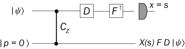
Fig. 1: Elementary teleportation circuit for continuous-variable cluster computation.

In this elementary teleportation circuit, the “input state” of mode 1, $|\psi\rangle$, is coupled to a zero-momentum eigenstate of mode 2, $|p=0\rangle=\int dx|x\rangle/\sqrt{\pi}$, via a continuous-variable controlled-$Z$ gate, $C_{Z}=\exp(2i\hat{x}\otimes\hat{x})$. Further, we use the Fourier transform, $F=\exp[i(\pi/2)(\hat{x}^{2}+\hat{p}^{2})]$, where $F|x\rangle=\int dye^{2ixy}|y\rangle/\sqrt{\pi}=|p=x\rangle$, and an arbitrary operator diagonal in the computational (position) basis, $D=\exp[if(\hat{x})]$. The measurement of mode 1 is supposed to be a measurement of the position observable $\hat{x}$ with a classical outcome $s$. This classical result then appears in the “teleported state” of mode 2 through the position displacement operator $X(s)=\exp(-2is\hat{p})$, where $X(s)|x\rangle=|x+s\rangle$.

The most important feature of the elementary teleportation circuit is that the $C_{Z}$ gate commutes with any diagonal operator $D$. Therefore, we can consider an equivalent scheme where the operator $D$ acts upon the input state $|\psi\rangle$ before the $C_{Z}$ gate is applied to the two modes. In other words, the circuit in Fig. 1 is identical to a circuit where the state $|\psi^{\prime}\rangle=D|\psi\rangle$ is teleported onto mode 2 and the only operation between the $C_{Z}$ gate and the $x$-homodyne detector of mode 1 is the inverse Fourier transform $F^{\dagger}$. Using $|\psi^{\prime}\rangle=\int dx\psi^{\prime}(x)|x\rangle$ as the “input state” of mode 1, directly after the $C_{Z}$ gate, we obtain the two-mode state,

$$C_{Z}\,|\psi^{\prime}\rangle\otimes|p=0\rangle=\frac{1}{\sqrt{\pi}}\,\int dxdy\,\psi^{\prime}(x)\,e^{2ixy}\,|x\rangle|y\rangle\,,$$ (1)

where we also used $|x\rangle|y\rangle\equiv|x\rangle\otimes|y\rangle$. Now absorbing the inverse Fourier transform into the $x$-homodyne detector means that we will apply the projector $F|x\rangle\langle x|F^{\dagger}=|p=x\rangle\langle p=x|$ onto mode 1 and effectively project it onto the $p$-basis $\{F|x\rangle\}=\{|p=x\rangle\}$. For a measurement result $p=s$, the conditional state of mode 2 becomes

$$\frac{1}{\sqrt{\pi}}\,\int dxdy\,\psi^{\prime}(x)\,e^{2ix(y-s)}\,|y\rangle=X(s)F|\psi^{\prime}\rangle\,,$$ (2)

in agreement with Fig. 1. The crucial point in this circuit is that, now again equivalently assuming that the operator $D$ acts between the $C_{Z}$ gate and the $p$-homodyne detection, this operation $D$ can be also absorbed into the detector. Thus, for a given state $|\psi\rangle$ of mode 1, the “output state” of mode 2, $X(s)FD|\psi\rangle$, can be manipulated solely by choosing different measurement bases $\{D^{\dagger}|p\rangle\}$ corresponding to the observables $D^{\dagger}\hat{p}D$. By concatenating these elementary teleportation circuits one can generate output states of the form $\cdots X(s_{2})FD_{2}X(s_{1})FD_{1}|\psi\rangle$ and hence realize any single-mode unitary gate [5, 4]. Thereby it depends on the type of the desired operations $D_{j}$ (Clifford or non-Clifford) how easily the position-displacements $X(s_{j})$ can be commuted through in order to be corrected. Moreover, the momentum-squeezed resource states will always be finitely squeezed (instead of being infinitely squeezed, unphysical zero-momentum eigenstates). This ultimately leads to distortions of the states that are teleported through the cluster [5]. These distortions might be suppressed for the case of Clifford (Gaussian) operations by exploiting parallelism and postselection [5].

Let us finally mention that an elementary teleportation circuit analogous to the one in Fig. 1 can be constructed where the resource state is a zero-position eigenstate $|x=0\rangle$, the operator $D$ is diagonal in the $p$ basis, $D=\exp[if(\hat{p})]$, the controlled phase gate has the form $\exp(2i\hat{p}\otimes\hat{p})$, the measurement after the inverse Fourier transform is a $p$ measurement with classical result $p=t$, and the output state contains a momentum-displacement $Z(-t)=\exp(-2it\hat{x})$, where $Z(t)|p\rangle=|p+t\rangle$.

4 Linear clusters for single-mode evolutions

The teleportation circuit described in the preceding section is the elementary building block for any cluster computation including both single-mode and multi-mode gates [14, 5]. In general, in order to apply a multi-mode gate via a cluster state, the input state must propagate through a nonlinear cluster. In the continuous-variable case, highly squeezed light modes can be coupled via QND-type controlled-$Z$ operations in order to create the required graph state [5]. In the following, however, we will focus on linear cluster states where each node has at most two links. Linear cluster states are a sufficient resource to implement arbitrary single-qubit or single-mode transformations. In the continuous-variable case, for some input state of mode 1, $|\psi\rangle$, an arbitrary single-mode evolution can be realized by teleporting the state through a linear chain of modes which are all coupled via $C_{Z}$ gates just as the two modes in the elementary two-mode teleportation circuit (see Fig. 2).

When using the linear $N$-mode cluster state in Fig. 2 for single-mode transformations, at each step $j$, an appropriate observable $\hat{p}^{\prime}_{j}=D_{j}^{\dagger}\hat{p}_{j}D_{j}$ must be measured yielding a set of $N-1$ classical results $p^{\prime}_{j}=s_{j}$. The corresponding position-displacements $X(s_{j})$ which appear in the output state of mode $N$ can be corrected at the end. For Clifford operations, by definition, we can always write

$$D_{j}U_{\rm WH}=U^{\prime}_{\rm WH}D_{j}\,,$$ (3)

where $D_{j}$ is the desired Clifford group operation, $U_{\rm WH}$ is a Weyl-Heisenberg (WH) group transformation [a phase-space displacement such as $X(s)$ or $Z(t)$] effected through previous cluster computations, and $U^{\prime}_{\rm WH}$ is a modified WH group transformation which can be undone for correcting the output state. Note that the desired operation $D_{j}$ remains unchanged here and only the WH transformation is modified. In this case, for example, we obtain $\cdots X(s_{2})FD_{2}X(s_{1})FD_{1}|\psi\rangle=\cdots X(s_{2})U^{\prime}_{\rm WH}(s_{1})FD_{2}FD_{1}|\psi\rangle$, if $D_{2}$ is an element of the Clifford group (the Fourier transform also belongs to the Clifford group). The WH transformations can then be corrected or further commuted through.

However, in the case of non-Clifford (non-Gaussian) operations $D_{j}$, the correct choice of measurement bases depends on the outcome of previous measurements, because only via this feedforward is it possible to commute through and correct the position displacements. As a result, the parallelism for Clifford operations, i.e., the feature that all measurements can be performed simultaneously, no longer holds for non-Clifford gates.

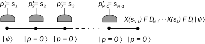
Fig. 2: Using linear Gaussian cluster states for single-mode evolutions: a chain of coupled squeezed modes is generated via controlled-$Z$ gates; an “input state” $|\psi\rangle$ can be teleported through the cluster and potentially manipulated at each step; the form of the output state depends on the choice of measurement bases for detecting the observables $\hat{p}^{\prime}_{j}=D_{j}^{\dagger}\hat{p}_{j}D_{j}$.

In the non-Clifford case, we have

$$D^{\prime}_{j}U_{\rm WH}=U_{\rm WH}D_{j}\,,$$ (4)

where now the desired non-Clifford operation $D_{j}$ can be, in general, only applied to the output state if the measurement basis is chosen such that in the current cluster computation, a modified $D^{\prime}_{j}$ will be added to the incoming states. In general, this modified $D^{\prime}_{j}$ will depend on the measurement results of the previous cluster computations (contained in $U_{\rm WH}$). More specifically, when combining two elementary cluster circuits (using a linear 3-mode cluster state), the output state becomes

$$|\psi\rangle_{\rm out} = X(s_{2})FD_{2}^{\prime}X(s_{1})FD_{1}|\psi\rangle\,,$$ (5)

where $D_{1}$ is due to the first circuit with a measurement of $D_{1}^{\dagger}\hat{p}D_{1}$ and $D_{2}^{\prime}\equiv D_{2}^{\prime}(\kappa,s_{1})$ is due to the second circuit with a measurement of $D_{2}^{\prime\dagger}\hat{p}D_{2}^{\prime}$. This can be rewritten as

$$|\psi\rangle_{\rm out} = X(s_{2})Z(s_{1})FD_{2}FD_{1}|\psi\rangle\,,$$ (6)

with $D_{2}^{\prime}(\kappa,s_{1})X(s_{1})=X(s_{1})D_{2}(\kappa)$ for a (desired) non-Clifford group operation $D_{2}\equiv D_{2}(\kappa)$. For example, in order to effect the cubic gate $D_{2}(\kappa)=e^{i\kappa\hat{x}^{3}}$, we have to measure the observable $D_{2}^{\prime\dagger}(\kappa,s_{1})\hat{p}D_{2}^{\prime}(\kappa,s_{1})$ of mode 2 with $D_{2}^{\prime}(\kappa,s_{1})=e^{3i\kappa s_{1}\hat{x}(s_{1}-\hat{x})}D_{2}(\kappa)$.

5 Gaussian single-mode evolutions: single-mode squeezer

In this section, we will now discuss an example for implementing a single-mode evolution using a linear Gaussian cluster state. Apart from the Gaussian cluster state, we also assume that all the measurements will be Gaussian measurements corresponding to homodyne detections. In other words, the argument of the diagonal operators $D$ will be, at most, of quadratic order in $\hat{x}$. Since an operator $D$ that contains a linear function of $\hat{x}$ is a momentum-displacement operator, measuring $D^{\dagger}\hat{p}D$ in this case simply means that the measured $p$ value must be shifted correspondingly. In our example, we will use operators of quadratic form, $D=e^{i\kappa\hat{x}^{2}}$. With these operators, we can realize a single-mode squeezer. A single-mode squeezer is an important primitive for performing Gaussian transformations. In fact, any multi-mode Gaussian transformation can be decomposed into a passive linear-optics network, a set of single-mode squeezers, and another linear-optics circuit [7]. When implementing a single-mode squeezing transformation via a Gaussian cluster state, we encounter the typical feature of Clifford parallelism. Moreover, via a sufficiently long but fixed cluster state we may still achieve universal squeezing.

In our example of a single-mode squeezer, the desired total Clifford group operation acting on the state $|\psi\rangle$ is described by $U=e^{r(\hat{a}^{2}-\hat{a}^{\dagger 2})/2}=e^{ir(\hat{x}\hat{p}+\hat{p}\hat{x})}$ with a squeezing parameter $r$. We may realize this operation by combining four elementary cluster circuits using a linear five-mode cluster state (see Fig. 2 with $N=5$). In each step $j=1...4$, the operation $X(s_{j})FD_{j}$ with $D_{j}\equiv D(\kappa_{j})\equiv e^{i\kappa_{j}\hat{x}^{2}}$ is applied. As a result, after correcting the phase-space displacements $X(s_{j})$, the output state of mode 5 will be $FD_{4}FD_{3}FD_{2}FD_{1}|\psi\rangle$. Now by choosing $\kappa_{1}=\kappa_{2}=\kappa$, we obtain $FD_{2}FD_{1}=F^{2}e^{i\kappa\hat{p}^{2}}e^{i\kappa\hat{x}^{2}}$. Up to rotations and higher-order terms in $\kappa$, this already corresponds to a single-mode squeezing operation, since $e^{i\kappa\hat{p}^{2}}e^{i\kappa\hat{x}^{2}}=e^{i\kappa(\hat{x}^{2}+\hat{p}^{2})}e^{i\kappa^{2}(\hat{x}\hat{p}+\hat{p}\hat{x})/2}+{\rm O}(\kappa^{3})$. However, by further applying $FD_{4}FD_{3}=F^{2}e^{-i\kappa\hat{p}^{2}}e^{-i\kappa\hat{x}^{2}}$ with $\kappa_{3}=\kappa_{4}=-\kappa$, we can add more squeezing and at the same time undo the unwanted rotations, because now we have $e^{-i\kappa\hat{p}^{2}}e^{-i\kappa\hat{x}^{2}}=e^{i\kappa^{2}(\hat{x}\hat{p}+\hat{p}\hat{x})/2}e^{-i\kappa(\hat{x}^{2}+\hat{p}^{2})}+{\rm O}(\kappa^{3})$. Thus, the effective total operation will be

$$FD_{4}FD_{3}FD_{2}FD_{1}=F^{2}e^{-i\kappa\hat{p}^{2}}e^{-i\kappa\hat{x}^{2}}F^{2}e^{i\kappa\hat{p}^{2}}e^{i\kappa\hat{x}^{2}}=e^{i\kappa^{2}(\hat{x}\hat{p}+\hat{p}\hat{x})}+{\rm O}(\kappa^{3})\,,$$ (7)

up to a global sign. This is approximately a single-mode squeezer with squeezing $r\equiv\kappa^{2}$. It leads to some squeezing in the position, $\hat{x}_{\rm out}=(1-\kappa^{2})\hat{x}+{\rm O}(\kappa^{3})$, and the corresponding antisqueezing in the momentum, $\hat{p}_{\rm out}=(1+\kappa^{2})\hat{p}+{\rm O}(\kappa^{3})$.

In the above protocol, the measurement bases do not change depending on the results of earlier measurements, because the desired output operation is a Clifford group operation. We explicitly demonstrate this for modes 1 and 2.

When combining two elementary clusters, as described before, and detecting $D_{j}^{\dagger}\hat{p}_{j}D_{j}$ of modes 1 and 2 with measurement results $s_{1}$ and $s_{2}$, mode 3 will be projected onto the state $X(s_{2})FD_{2}X(s_{1})FD_{1}|\psi\rangle$. Since $D_{2}$ is an element of the Clifford group, the correction based on the result of the first measurement, $X(s_{1})$, can be commuted through the $D_{2}$-operation, $D_{2}X(s_{1})=Z(\kappa s_{1})X(s_{1})D_{2}$ (up to a global phase). Note that here the desired Clifford group operation $D_{2}$ remains unchanged, while the WH group elements necessary for correction become modified. This is why also the detection of mode 2 is just a measurement of $D_{2}^{\dagger}\hat{p}_{2}D_{2}$ independent of the result of the first measurement of mode 1. So finally, the resulting state

$$|\psi^{\prime}\rangle = X(s_{2})FZ(\kappa s_{1})X(s_{1})D_{2}FD_{1}|\psi\rangle$$ (8)

$$= X(s_{2}-\kappa s_{1})Z(s_{1})F^{2}e^{i\kappa\hat{p}^{2}}e^{i\kappa\hat{x}^{2}}|\psi\rangle$$

can be corrected to obtain the desired transformation, as described above. The remaining operations in order to complete the single-mode squeezer can be similarly corrected.

In the scheme described above, measuring the observables $\hat{p}^{\prime}_{j}=D_{j}^{\dagger}\hat{p}_{j}D_{j}$ (instead of $\hat{p}_{j}$) for $D_{j}\equiv e^{i\kappa_{j}\hat{x}^{2}}$ means that a linear combination of position and momentum should be detected, $\hat{p}^{\prime}_{j}=\hat{p}_{j}+\kappa_{j}\hat{x}_{j}$. This, however, simply corresponds to the measurement of rotated quadratures, $(\hat{p}_{j}\cos\theta_{j}-\hat{x}_{j}\sin\theta_{j})/(\cos\theta_{j})$ with $\kappa_{j}\equiv-\tan\theta_{j}$, where the measurement results must be rescaled by the factor $\cos\theta_{j}$. Thus, solely by adjusting the local oscillator phase $\theta_{j}=\tan^{-1}(-\kappa_{j})$ of the homodyne detectors, we can measure any observable $\hat{p}^{\prime}_{j}=D_{j}^{\dagger}\hat{p}_{j}D_{j}$ and no additional squeezers are required in front of the detectors. This property, of course, does not only apply to the cluster scheme for the single-mode squeezer. Any multi-mode Gaussian transformation can be performed via a given cluster state solely by doing suitable homodyne measurements [5].

In the realistic case, finitely squeezed resources are used in order to build the linear five-mode cluster state. When realizing the single-mode squeezing transformation via this finitely squeezed cluster state, at each of the four measurement steps extra noise will be added to the output state, thus distorting the desired squeezing transformation appearing in mode 5. However, since the desired operation is a Clifford group operation, parallelism and postselection could be used to suppress the effect of these distortions [5]. In this case, modes 3 and 4 are measured before the $2-5$ cluster state is attached to mode 1 which is in the input state $|\psi\rangle$. For the final attachment and detections of modes 1 and 2, only those $2-5$ cluster states will be postselected which lead to the smallest distortions of the transformed input state. The efficiency of this method depends on the form of the input state $|\psi\rangle$ and hence on the encoding used in the cluster computation [5].

Using a linear Gaussian cluster state, we may now apply some squeezing $r\equiv\kappa^{2}$ to the input state $|\psi\rangle$. For a sufficiently long linear cluster state, we may repeat this procedure and gradually add more squeezing. However, the degree of output squeezing in $|\psi\rangle_{\rm out}$ can be controlled solely through the choice of the detection bases without ever changing the cluster state. For example, if we decide to apply only little squeezing to the state $|\psi\rangle$, most of our measurements will be simple $p$-detections in order to propagate the state through the cluster. Different squeezing transformations can be performed using the same fixed cluster state but different homodyne measurements. This kind of universality is the typical feature of cluster-computation. In the next section, we will compare this and other properties of cluster-computation with those of “off-line schemes”.

6 Comparison to off-line schemes

Various continuous-variable schemes have been proposed in which particular transformations (gates) are applied to some input state via a suitably prepared off-line resource state [17, 20, 21, 22]. In a teleportation-based continuous-variable off-line scheme, similar to that for discrete variables and single-photon states [16], an entangled two-mode squeezed state is modified beforehand in order to apply a desired transformation to some input state via quantum teleportation [17]. In the limit of infinite squeezing, the two-mode squeezed state corresponds to the output of a symmetric beam splitter with the two inputs $|p=0\rangle$ and $F^{\dagger}|p=0\rangle=|x=0\rangle$ (see Fig. 3). Note that the infinitely squeezed two-mode squeezed state $\int dx|x\rangle|x\rangle/\sqrt{\pi}$ is equivalent to a two-mode cluster state, $e^{2i\hat{x}\otimes\hat{x}}|p=0\rangle|p=0\rangle=\int dx|p=x\rangle|x\rangle/\sqrt{\pi}$ up to a local Fourier transform.

Quantum teleportation of an input state $|\psi\rangle$ is achieved by combining the input mode with one half of the two-mode squeezed state (mode 1) at a second symmetric beam splitter [23] (Fig. 3). Via $x$ and $p$ homodyne detections at the two output ports, the linear combinations $u=x_{\rm in}-x_{1}$ and $v=p_{\rm in}+p_{1}$ can be determined. Depending on these classical measurement results, the conditional state of mode 2 (the other half of the entangled state) becomes a replica of the input state $|\psi\rangle$ up to known position and momentum displacements, $X(-u)Z(-v)|\psi\rangle$ [24].

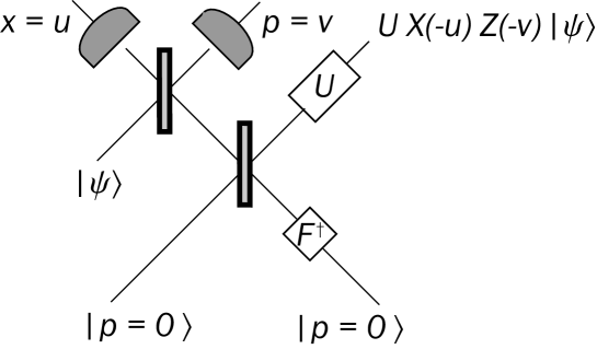
Fig. 3: Off-line transformation of a quantum state $|\psi\rangle$ via continuous-variable quantum teleportation using a suitably modified two-mode squeezed state (here in the limit of infinite squeezing).

Now consider the situation where the position and momentum displacements in the output state $X(-u)Z(-v)|\psi\rangle$ are not corrected and another unitary transformation $U$ is applied to the state of mode 2, $UX(-u)Z(-v)|\psi\rangle$. This scenario is equivalent to a scheme in which the unitary transformation $U$ is performed before any measurements are done. In other words, the two-mode squeezed state gets modified before it is used as a resource for quantum teleportation, $\int dx|x\rangle|x\rangle/\sqrt{\pi}\rightarrow(\mbox{1$\!\!${\large 1}}\otimes U)\int dx|x\rangle|x\rangle/\sqrt{\pi}$. Now if $U$ is an element of the Clifford group, we can again write $UX(-u)Z(-v)=U^{\prime}_{\rm WH}(u,v)U$ where $U^{\prime}_{\rm WH}$ is a modified WH group transformation, but the desired $U$ is unchanged. Thus, after correcting the known displacements $U^{\prime}_{\rm WH}$, we can generate the output state $U|\psi\rangle$. In this way, quantum gates can be applied on-line via quantum teleportation [15] after the corresponding gate has been applied off-line to the entanglement resource. The scheme described here is just the continuous-variable version of this method [17]. For example, if the desired transformation $U$ is a single-mode squeezer that generates $\hat{x}_{\rm out}=e^{-r}\hat{x}$ and $\hat{p}_{\rm out}=e^{+r}\hat{p}$, then we have $UX(-u)Z(-v)|\psi\rangle=X(-e^{-r}u)Z(-e^{+r}v)U|\psi\rangle$ which can be easily corrected to obtain $U|\psi\rangle$.

Note that in order to preserve the set of tools needed in the actual on-line teleportation scheme (homodyne detections and displacements), it is necessary that $U$ is an element of the Clifford group. If $U$ is not an element of the Clifford group, we would have to apply a different $U^{\prime}$ to the entanglement resource in order to be able to correct the teleported state via simple phase-space displacements and still effect the desired gate $U$, since then $U^{\prime}U_{\rm WH}=U_{\rm WH}U$. However, in this case, $U^{\prime}$ will depend on the classical results of the homodyne detections $u$ and $v$ during the on-line teleportation protocol (contained in $U_{\rm WH}$). As a result, we can no longer apply the correct $U^{\prime}$ off-line to the entanglement resource before the on-line teleportation. The complications that arise here in the non-Clifford case are similar to those in cluster-state computation. However, in cluster computation, we can still apply the correct non-Clifford $D_{j}$ in every step $j$, because this can be achieved by choosing the right measurement basis depending on the measurement results in previous steps.

In order to obey the rules of “off-line computation”, we must apply the desired gate operation $U$ off-line before the on-line teleportation. Therefore, the resulting teleported state will always be of the form $UX(-u)Z(-v)|\psi\rangle$. Now even if $U$ is not an element of the Clifford group, it can be commuted through the phase-space displacements. However, in this case, the correction operation will become more complicated than simple displacements. In general, if $U_{k}$ describes an interaction of $k$th order in $\hat{x}$ and $\hat{p}$, we have $U_{k}U_{\rm WH}=U_{k-1}U_{k}$ ($k>1$) where $U_{k-1}$ is a known interaction of $(k-1)$th order depending on the form of $U_{\rm WH}$ [17]. Thus, if we allow for more complicated correction operations than simple phase-space displacements, we may still teleport a non-Clifford operation onto the state $|\psi\rangle$. For example, a cubic gate $U_{3}$ would require a correction operation of the form $U_{2}$ which is a Clifford (Gaussian) operation and includes displacements and squeezers [17].

In Sec. 2, we mentioned various aspects in which cluster computation and off-line schemes differ. For example, the essence of implementing a teleportation-based off-line scheme is that the “difficult” operations are performed off-line. In the above continuous-variable protocol such a “difficult” operation $U$ is applied off-line to a two-mode squeezed state. This off-line operation could be, for instance, a cubic phase gate, while during the on-line teleportation protocol Gaussian operations are sufficient. Compare this with a cubic gate realized via a continuous-variable cluster state. In this case, Gaussian (Clifford) operations suffice in order to build the cluster off-line. However, a non-Gaussian measurement is required on-line to accomplish the cubic gate. This could be realized, for example, by putting a cubic gate in front of the $p$-homodyne detector.

When implementing Clifford gates for continuous variables, off-line and cluster-based schemes compare as follows. Consider as the desired gate a single-mode squeezing transformation. In the off-line scheme, assume that we are given a highly squeezed two-mode squeezed state for free. Now the “difficult” operation would be to apply the single-mode squeezing transformation $U$ off-line to the two-mode squeezed state. Eventually, this single-mode squeezing $U$ can be teleported onto some input state via fixed homodyne detections and conditional phase-space displacements. In contrast, given a highly squeezed linear Gaussian cluster state, no further manipulation of this resource is needed off-line. However, for the on-line measurements, as described in the preceding section, we have to detect “squeezed quadratures”, i.e., observables of the form $D^{\dagger}\hat{p}D$ where $D$ represents a quadratic gate. This could be realized by putting a single-mode squeezer (plus phase shifters) in front of the $p$-homodyne detector. Of course, such an approach would be awkward, because the measurement of $D^{\dagger}\hat{p}D$ in this case only requires adjustment of the homodyne detector’s local oscillator phase. However, this example illustrates the conceptual difference between the off-line and the cluster scheme: in the former, squeezing is applied off-line depending on the desired output squeezing and the homodyne measurements are fixed; in the latter, the cluster state is fixed and the measured observables are “squeezed” depending on the desired output squeezing.

As a consequence, in cluster computation, in general, deciding the final transformation can be postponed until the very end. This leads to another conceptual difference between cluster and off-line schemes, namely universality. What kind of gates can be realized via a given cluster or off-line state? If the cluster state is sufficiently large, any gate or gate sequence is realizable via the same cluster state only by adjusting the measurement bases. An off-line entangled state must be correspondingly modified for implementing particular gates and different off-line states must be selected for different computations. For example, when performing the single-mode squeezing transformation via a (sufficiently long) linear Gaussian cluster state, we may still decide how much squeezing we apply after the cluster state has been created. In the case of a teleportation-based off-line scheme, we have to apply the corresponding amount of squeezing to the entangled state (or select a suitable set of modified entangled states) before the on-line protocol.

Finally, let us compare the different types of input states in cluster and off-line computation. Typically, in cluster computation, the “input state” will be some fixed blank state which is part of the cluster. In contrast, in the teleportation-based off-line protocol, an arbitrary input state is coming independently from outside and is coupled to one half of the entangled resource state only during the on-line computation. This coupling will be performed only provided the resource state has been suitably prepared. Of course, one may consider a situation where also a cluster state is only attached to some input state (which could be part of some other cluster state) during the on-line computation. In fact, such a scenario turns out to be useful when implementing Gaussian operations via Gaussian cluster states due to the Clifford parallelism [5]. In this case, some of the homodyne measurements can be made before the cluster state is attached to the input state or another cluster state. Similar to off-line computation schemes, only those cluster states would be postselected which are best suited to effect the desired transformation (and least likely to distort the input state).

7 Conclusion

In summary, we briefly described the concept of continuous-variable cluster computation using Gaussian cluster states. As an example of Gaussian cluster computation, we considered a single-mode squeezer. This example is particularly simple, because it represents a single-mode evolution which can be realized via linear cluster states. Moreover, the desired operation in this case is a Clifford (Gaussian) operation. As a result, during the computation, the measurement bases do not change depending on the results of earlier measurements. In this case, all measurements in the cluster computation can be performed at the same time. Finally, we discussed some conceptual similarities and differences between cluster-computation and off-line computation and illustrated these for the case of continuous variables.

References

- [1] M. A. Nielsen and I. L. Chuang, Quantum Computation and Quantum Information, Cambridge University Press (2000).
- [2] R. Raussendorf and H. J. Briegel, Phys. Rev. Lett. 86, 5188 (2001).
- [3] S. L. Braunstein and P. van Loock, Rev. Mod. Phys. 77, 513 (2005).
- [4] S. Lloyd and S. L. Braunstein, Phys. Rev. Lett. 82, 1784 (1999).
- [5] N. C. Menicucci, P. van Loock, M. Gu, C. Weedbrook, T. C. Ralph, and M. A. Nielsen, eprint: quant-ph/0605198 (2006).
- [6] J. Zhang and S. L. Braunstein, Phys. Rev. A 73, 032318 (2006).
- [7] S. L. Braunstein, Phys. Rev. A 71, 055801 (2005).
- [8] D. F. Walls and G. J. Milburn, Quantum Optics, Springer, Berlin (1994).
- [9] J.-P. Poizat, J. F. Roch, and P. Grangier, Ann. Phys. (Paris) 19, 265 (1994).
- [10] B. Julsgaard, A. Kozhekin, and E. S. Polzik, Nature (London) 413, 400 (2001).
- [11] J. M. Geremia, J. K. Stockton, and H. Mabuchi, Science 304, 270 (2004).
- [12] M. A. Nielsen, Phys. Rev. Lett. 93, 040503 (2004).
- [13] D. E. Browne and T. Rudolph, Phys. Rev. Lett. 95, 010501 (2005).
- [14] M. A. Nielsen, Rep. Math. Phys. 57, 147 (2006).
- [15] D. Gottesman and I. L. Chuang, Nature (London) 402, 390 (1999).
- [16] E. Knill, R. Laflamme and G. J. Milburn, Nature 409, 46 (2001).
- [17] S. D. Bartlett and W. J. Munro, Phys. Rev. Lett. 90, 117901 (2003).
- [18] P. Walther, K. J. Resch, T. Rudolph, E. Schenck, H. Weinfurter, V. Vedral, M. Aspelmeyer, and A. Zeilinger, Nature (London) 434, 169 (2005).
- [19] X. Zhou, D. W. Leung, and I. L. Chuang, Phys. Rev. A 62, 052316 (2000).
- [20] D. Gottesman, A. Kitaev, and J. Preskill, Phys. Rev. A 64, 012310 (2001).
- [21] R. Filip, P. Marek, and U. L. Andersen, Phys. Rev. A 71, 042308 (2005).
- [22] A. M. Lance, H. Jeong, N. B. Grosse, T. Symul, T. C. Ralph, and P. K. Lam, Phys. Rev. A 73, 041801 (R) (2006).
- [23] S. L. Braunstein and H. J. Kimble, Phys. Rev. Lett. 80, 869 (1998).
- [24] usually, the quantum optical phase-space displacement operator is used to describe the displacements in “Alice’s” measurement basis and “Bob’s” correction operation for continuous-variable quantum teleportation. Here we prefer to stick to the WH group elements, where differs from only by a global phase with . Alice’s measurement basis is then described by . Bob’s correction operation would be in this case. In a communication rather than computation scenario where Alice and Bob are spatially separated, of course, Alice needs to send the results and to Bob via a classical channel.