Backward Evolving Quantum States

Abstract

The basic concept of the two-state vector formalism, which is the time symmetric approach to quantum mechanics, is the backward evolving quantum state. However, due to the time asymmetry of the memory’s arrow of time, the possible ways to manipulate a backward evolving quantum state differ from those for a standard, forward evolving quantum state. The similarities and the differences between forward and backward evolving quantum states regarding the no-cloning theorem, nonlocal measurements, and teleportation are discussed. The results are relevant not only in the framework of the two-state vector formalism, but also in the framework of retrodictive quantum theory.

I Introduction

In 1964 Aharonov, Bergmann, and Lebowitz (ABL) ABL laid the foundations for the Time Symmetric Formalism of Quantum Mechanics. The basic idea of the formalism is the introduction of a quantum state evolving backward in time in addition to the standard quantum state evolving forward in time. The formalism uncovered numerous peculiar features of quantum mechanics.

One peculiarity is that some particular pre- and post-selections lead to situations in which we know with certainty the result of some intermediate measurement, even though neither pre-selection nor post-selection are eigenstates of the corresponding variable. I have named such definite outcomes “elements of reality” ER . It is possible for pre- and post-selected systems to yield simultaneous elements of reality for noncommuting observables XYZ . Even more surprisingly, it is possible to obtain seemingly contradictory elements of reality, such as a single ball which is to be found with certainty, if searched for, in any one of two or more distinct locations AV1991 .

The most important result of the two-state vector formalism is related to “weak measurements” performed on pre-and post-selected systems. The outcomes of weak measurements (named weak values), which are given by a simple universal expression, may turn out to be far from the range of eigenvalues of the corresponding operator AV1990 .

The backward evolving state is a premise not only of the two-state vector formalism, but also of “retrodictive” quantum mechanics retro , which deals with the analysis of quantum systems based on a quantum measurement performed in the future relative to the time in question.

In this paper I shall not discuss the advantages of the two-state vector and the retrodictive approaches. Rather, I consider here a theoretical question: what are the limitations on the possible manipulations of a backward evolving quantum state? In the following sections I will analyze, in particular, the possibility of cloning and teleporting backward evolving quantum states. I will touch upon these questions also with regard to two-state vectors, which include both forward and backward evolving states.

First, however, I would like to take advantage of the opportunity to give tribute to GianCarlo Ghirardi and to express my view on the Quantum Universe. In the next section I will explain how this view is related to the backward evolving quantum state.

II The Quantum Universe

There is no consensus regarding the Quantum Universe. Without having seen other contributions, I take the risk of predicting that the multitude of views presented here will show this very vividly.

The followers of Bohr forbid us to talk about the Quantum Universe: quantum theory is not to tell us the story of “reality”. I believe, however, that science must tell us what the Universe is as well as how it behaves. If quantum theory does not describe our world, then what does? No other theory agrees so well with experimental evidence.

For those who do wish to understand the Universe - and to accept that it is quantum - the central question becomes: what is the status, or physical meaning, of the quantum state, of the quantum wave function? The Wave Function of the Universe, evolving according to the Schrodinger Equation with its numerous branches, seems very remote from the picture of the world as we experience it.

This connection is made via the idea that every measurement causes a collapse of the wave function. For, the collapsed wave function does resemble the world we know. When and how collapse occurs, however, is a very difficult issue. GianCarlo Ghirardi, together with Phillip Pearle, Riminy and Weber are the pioneers of physical proposals for the collapse process P ; GRW .

In the past, David Albert and I analyzed the Stern-Gerlach experiment within the framework of the Ghirardi-Rimini-Weber (GRW) collapse model AVGRW . We claimed that GRW-collapse does not occur during a carefully arranged measurement process, but Ghirardi and his collaborators showed that it does take place in the brain of the observer AVGRWrep . At that time David Albert persuaded me of the advantages of the many-worlds interpretation, although he has since come to favor the GRW type solution Al .

Another option is to deny that the collapse process exists and that the Schrodinger Wave corresponds to our experience. Bohm, de Broglie, and Bell suggested that the Schrodinger Wave is just a pilot wave of “Bohmian particle positions” and that those “particles” which have single trajectories draw the picture of our familiar world.

My strong preference remains to deny both the collapse process and the existence of additional ontological entities (i.e. Bohmian particle positions). I accept that the Wave Function of the Universe is all the physical ontology that exists. For this economy and elegance in physical laws I am prepared to pay the price of acknowledging that I and the world I see are not the only ones of the physical universe. There are numerous parallel worlds similar to the one I know, all incorporated in a single quantum State of the Universe myMWI . The parallel worlds are essentially irrelevant to me in this world. In theory, parallel worlds can interfere, but that this should be observable is not feasible.

I can trace back and understand my world in the past, but my (this branch) future consists of multiple worlds. For the purpose of describing a quantum system between two measurements it is convenient to consider a single world defined by the results of measurements both in the past and in the future relative the time I wish to discuss. Thus, I find it convenient to use the two-state vector formalism in the framework of the many-worlds interpretation. The concept of the two-state vector can be understood most clearly in a world with definite results of experiments both in the past and in the future.

III Backward Evolving Quantum State

There is an ongoing discussion about the meaning of the quantum state. I have also taken part in this discussion psi , but here I shall adopt a pragmatic approach. A quantum state represents a set of statements about the probabilities for the outcomes of measurements that can be explained in the framework of any interpretation of quantum mechanics. Let us spell out these probabilities for backward and forward evolving quantum states.

We consider a quantum system which is described completely by a variable $A$. At time $t$, an ideal measurement of $A$ is performed with the outcome $A=a$. Then, it is said, immediately after the measurement the system is described by the quantum state $|A=a\rangle$ (evolving forward in time). This outcome also tells us that immediately before the measurement the quantum state (evolving forward in time) was not orthogonal to $|A=a\rangle$.

It is possible also to apply retrodiction to the measurement of $A$ and say that immediately prior to the measurement there is an additional quantum state evolving backward in time $\langle A=a|$, see Fig. 1.

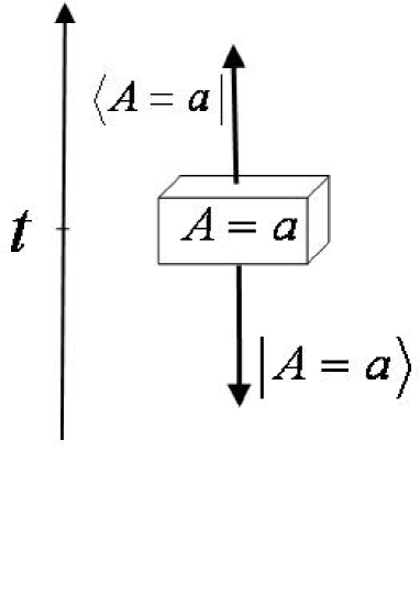
Figure 1: Measurement of $A$ at time $t$ creates the forward evolving quantum state $|A=a\rangle$ and the backward evolving quantum state $\langle A=a|$.

The operational meaning of the fact that a system is described at a particular time by the quantum state $|A=a\rangle$ evolving forward in time, is that a measurement of $A$ at that time yields $A=a$ with probability 1. This is irrespective of a post-selection of a particular outcome of a measurement performed after that time. (Note that cases in which another measurement of $A$ yields a different outcome are automatically disregarded, since a quantum system in the state $|A=a\rangle$, with the only interaction being another measurement of $A$, cannot yield any other outcome in the latter measurement of $A$.) Given that there is no post-selection, we can state also that the probability of obtaining $B=b$ in a measurement of another variable $B$ is given by the square of the scalar product $|\langle B=b|A=a\rangle|^{2}$.

Almost the same can be said about the operational meaning of describing a system at a particular time by the backward evolving quantum state $\langle A=a|$. A measurement of $A$ at that time yields $A=a$ with probability 1, irrespective of a pre-selection of a particular outcome of a measurement before that time. (Note that, again, cases in which we pre-select states orthogonal to $|A=a\rangle$ are automatically disregarded.) If there is no pre-selection, the probability of finding $B=b$ is given by the square of the scalar product $|\langle B=b|A=a\rangle|^{2}$.

Usually, at the “present” time there is no particular post-selection, but there is some pre-selection. In order to eliminate this pre-selection we have to “erase” the past of the quantum system. One way to achieve this is to cause the system to become completely entangled with another ancillary system, see Fig. 2. So long as the ancilla is not measured, the future of the ancilla is unknown and the past of the quantum system becomes unknown too. Thus it is possible for the probabilities of the results of a measurement at a particular time (after preparation of the entangled state and before the post-selection) to depend solely on the backward evolving state.

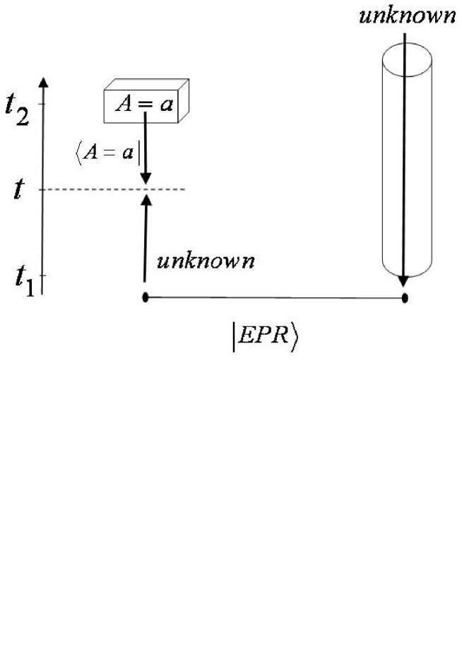
Figure 2: Erasure of the past of the particle with a backward evolving quantum state $\langle A=a|$. We prepare the EPR state of the particle and an ancilla and guard the ancilla such that it will not be measured.

A formal proof of the above claim might be helpful at this point. Consider two systems pre-selected in a completely entangled state $|\Psi_{ent}\rangle$. One of the systems is post-selected via a complete measurement whose outcome is $A=a$. We are looking for the probability of obtaining the particular outcome $B=b_{n}$ in an intermediate measurement of $B$. The probability of obtaining a particular outcome in a measurement performed on a pre- and post-selected system is given by the Aharonov-Bergmann-Lebowitz (ABL) formula ABL . Its generalization for partial post-selection V98 yields:

$${\rm Prob}(B=b_{n}) = {{||{\bf P}_{A=a}{\bf P}_{B=b_{n}}|\Psi\rangle_{ent}||^{2}}\over{\sum_{i}||{\bf P}_{A=a}{\bf P}_{B=b_{i}}|\Psi_{ent}\rangle||^{2}}}$$ (1)

$$= {{||~{}|A=a\rangle\langle A=a||B=b_{n}\rangle\langle B=b_{n}|\sum_{j}|B=b_{j}\rangle|j\rangle_{anc}||^{2}}\over{\sum_{i}||~{}|A=a\rangle\langle A=a||B=b_{i}\rangle\langle B=b_{i}|\sum_{j}|B=b_{j}\rangle|j\rangle_{anc}||^{2}}}$$

$$= {{||~{}|A=a\rangle\langle A=a|B=b_{n}\rangle|n\rangle_{anc}||^{2}}\over{\sum_{i}||~{}|A=a\rangle\langle A=a|B=b_{i}\rangle|i\rangle_{anc}||^{2}}}$$

$$= {{|~{}\langle A=a|B=b_{n}\rangle|^{2}}\over{\sum_{i}|\langle A=a|B=b_{i}\rangle|^{2}}}=|~{}\langle A=a|B=b_{n}\rangle|^{2}.$$

This shows the equivalence, in some sense, of a quantum state at present evolving forward in time when the future is unknown, and a quantum state evolving backward in time given that the past of the system is erased. “Erasing” the past is, in principle, a complicated procedure. It consists of preparing an entangled state of our system and an ancillary system, as well as of “guarding” the ancillary system against measurement. In many practical situations, however, nature provides the “erasing” for free. For example, the filament of a light bulb produces photons with an “erased” (for all practical purposes) polarization state. The photon polarization is entangled with the quantum state of the filament which cannot be measured using current technology. Leggett Leg called this process by a different name, “garbling sequence” or “coherence-destroying manipulation”, and mentioned that nature, in effect, does it for us all the time.

IV The Asymmetry of the Memory Time Arrow

We wish to analyze the similarities and the differences between forward and backward evolving quantum states, with regard to the possibilities for performing various manipulations. One similarity which we have already mentioned is that an ideal complete measurement at a particular time that yields $A=a$ creates both the quantum state $|A=a\rangle$ evolving forward in time and the quantum state $\langle A=a|$ evolving backward in time.

A notable difference between forward and backward evolving states has to do with the creation of a particular quantum state at a particular time. In order to create the quantum state $|A=a\rangle$ evolving forward in time, we measure $A$ before this time. We cannot be sure to obtain $A=a$, but if we obtain a different result $A=a^{\prime}$ we can always perform a unitary operation and thus create at time $t$ the state $|A=a\rangle$. On the other hand, in order to create the backward evolving quantum state $\langle A=a|$, we measure $A$ after time $t$. If we do not obtain the outcome $A=a$, we cannot repair the situation, since the correcting transformation has to be performed at a time when we do not yet know which correction is required. Therefore, a backward evolving quantum state at a particular time can be created only with some probability, while a forward evolving quantum state can be created with certainty. (Only if the forward evolving quantum state is identical to the backward evolving state we want to create at time $t$, and only if we know that no one touches the system at time $t$, can the backward evolving state be created with certainty, since then the outcome $A=a$ occurs with certainty. But this is not an interesting case.)

The formalism of quantum theory is time reversal invariant. It does not have an intrinsic arrow of time. The difference with regard to the creation of backward and forward evolving quantum state follows from the “memory’s” arrow of time. We can base our decision of what to do at a particular time only on events in the past, since future events are unknown to us. The memory time arrow is responsible for the difference in our ability to manipulate forward and backward evolving quantum states.

V Ideal Nondemolition Measurements and Teleportation

The same ideal (von Neumann) measurement procedure applies both to forward evolving quantum states and to backward evolving quantum states. In both cases, the outcome of the measurement is known after the time of the measurement. All that is known about what can be measured in an ideal (nondemolition) measurement of a forward evolving quantum state can be applied also to a backward evolving quantum state. The proof relies on the fact that the operational meaning of measurability for a forward evolving state, and that of measurability for a backward evolving state, are essentially the same: three consecutive measurements have to yield the same outcome.

There are constraints on the measurability of nonlocal variables, i.e. variables of composite systems with parts separated in space. When we consider instantaneous nondemolition measurements (i.e. measurements in which, in a particular Lorentz frame during an arbitrarily short time, local records appear which, when taken together, specify the eigenvalue of the nonlocal variable), we have classes of measurable and unmeasurable variables. For example, the Bell operator variable is measurable, while some other variables VP , including certain variables with product state eigenstates NLWE ; NLWEVG , cannot be measured.

The procedure for measuring nonlocal variables involves entangled ancillary particles and local measurements, and can get quite complicated. Fortunately, there is no need to go into detail in order to show the similarity of the results for forward and backward evolving quantum states. The operational meaning of the statement that a particular variable $A$ is measurable is that in a sequence of three consecutive measurements of $A$ - the first taking a long time and possibly including bringing separate parts of the system to the same location and then returning them, the second being short and nonlocal, and the third, like the first, consisting of bringing together the parts of the system - all outcomes have to be the same, see Fig. 3. But this is a time symmetric statement; if it is true, it means that the variable $A$ is measurable both for forward and backward evolving quantum states.

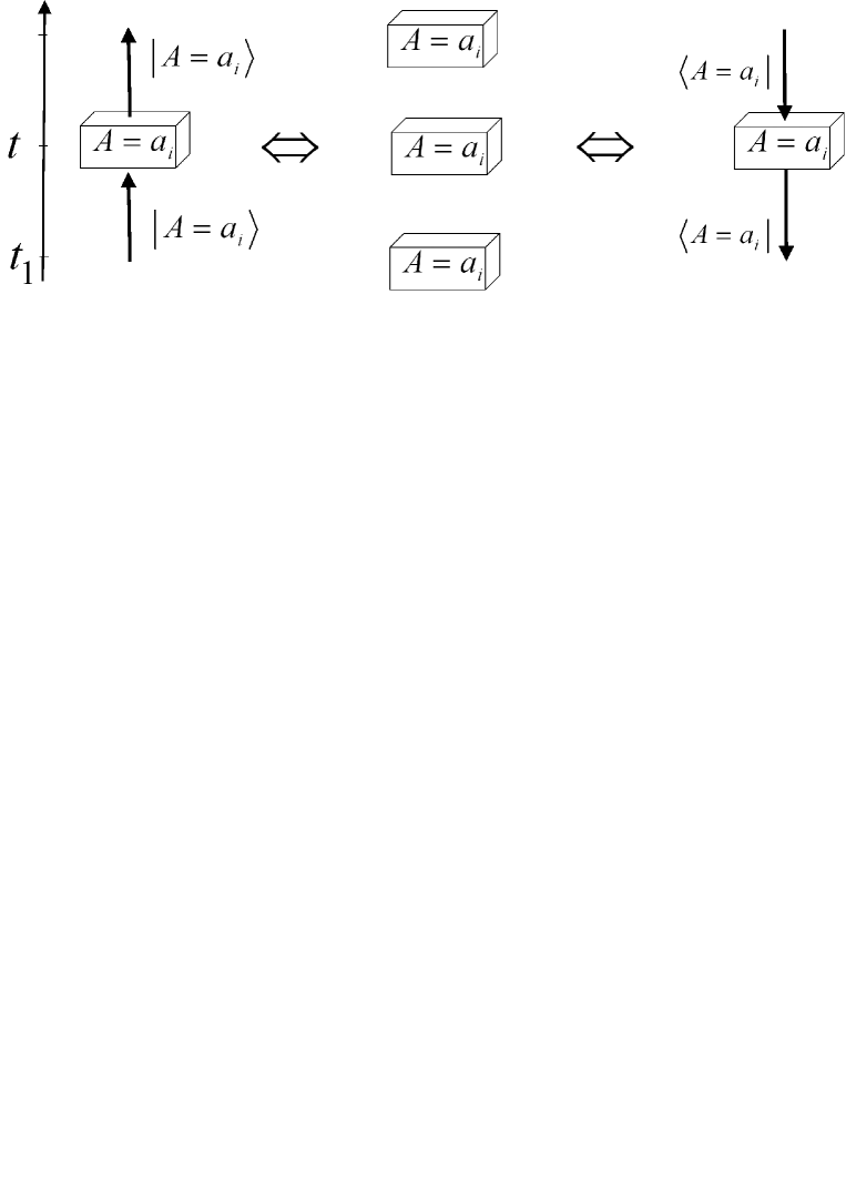
Figure 3: The operational meaning of creating a measuring device for a nondemolition measurement of $A$ at time $t$ means that the device and the two other measuring devices operating before and after time $t$ have to give the same eigenvalues of $A$. It is true both for forward and backward evolving quantum states.

We need also to obtain the correct probabilities in the case that different variables are measured at different times. For a forward evolving quantum state it follows directly from the linearity of quantum mechanics. For a backward evolving quantum state, the simplest argument is the consistency between the probability of the final measurement, which is now $B=b$, given the result of the intermediate measurement $A=a$, and the result of the intermediate measurement given the result of the final measurement. We assume that the past is erased. The expression for the former is $|~{}\langle A=a|B=b\rangle|^{2}$. For consistency, the expression for the latter must be the same, but this is what we need to prove.

In exactly the same way we can show that the same procedure for teleportation of a forward evolving quantum state tele yields also teleportation of a backward evolving quantum state. As the forward evolving quantum state is teleported to a space-time point in the future light cone, the backward evolving quantum state is teleported to a point in the backward light cone. Indeed, the operational meaning of teleportation is that the outcome of a measurement in one place is invariably equal to the outcome of the same measurement in the other place. Thus, the procedure for teleportation of the forward evolving state to a point in the future light cone invariably yields teleportation of the backward evolving quantum state to the backward light cone.

Let us consider an experiment demonstrating teleportation of a backward evolving quantum state. Victoria performs a measurement of $B$ and gives the quantum system to Alice. Alice teleports the quantum state in the usual way to Bob who gives the state to Victor. Victor measures $A$ and selects all cases in which he obtains $A=a$. For these cases he asks Victoria for her measurement outcomes. The outcomes should respect the probability law $p(B=b)=|\langle B=b|A=a\rangle|^{2}$. In particular, when $B=A$, Victoria always (in all the cases in which Victor asks her) gets $A=a$.

The impossibility of teleportation of the backward evolving quantum state outside the backward light cone follows from the fact that it will lead to teleportation of the forward evolving quantum state outside the forward light cone, and this is impossible since it obviously breaks causality.

VI Demolition Measurements

The argument used above does not answer the question of whether it is possible to measure nonlocal variables in a demolition measurement. Obviously, a demolition measurement of a nonlocal variable of a quantum state evolving forward in time does not measure this variable for a quantum state evolving backward in time. Any nonlocal variable of a composite system can be measured with demolition for a quantum state evolving forward in time V . Recently, it has been shown VN also that any nonlocal variable can be measured for a quantum state evolving backward in time. Moreover, the procedure is simpler and requires fewer entanglement resources.

The difference follows from the fact that we can change the direction of time evolution of a backward evolving state along with flipping it, see Fig. 4. Indeed, all we need is to prepare an EPR state of our system and an ancilla. Guarding the system and the ancilla ensures that the forward evolving quantum state of the ancilla is the flipped state of the system. For a spin wave function we obtain $\alpha\langle{\uparrow}|+\beta\langle{\downarrow}|\rightarrow-\beta^{\ast}|{\uparrow}\rangle+\alpha^{*}|{\downarrow}\rangle$. For a continuous variable wave function $\Psi(q)$ we need the original EPR state $|q-\tilde{q}=0,~{}~{}p+\tilde{p}=0\rangle$. Then, the backward evolving quantum state of the particle will transform into a complex conjugate state of the ancilla $\Psi(q)\rightarrow\Psi^{\ast}(\tilde{q})$.

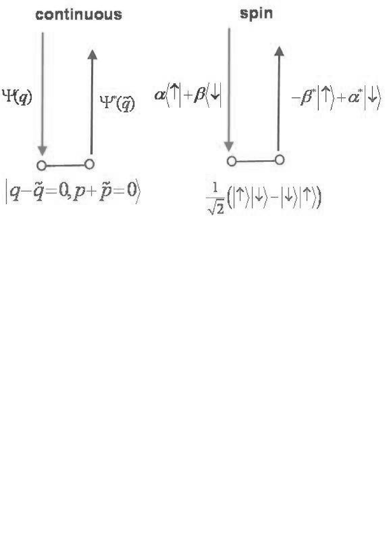
Figure 4: The backward evolving state can be transformed to “flipped” state evolving forward in time.

If the particle and the ancilla are located in different locations, then such an operation is a combination of time reversal and teleportation of a backward evolving quantum state of a continuous variable V94 .

We cannot flip and change the direction of time evolution of a quantum state evolving forward in time. To this end we would have to perform a Bell measurement on the system and the ancilla and to get a particular result (singlet). However, we cannot ensure this outcome, nor can we correct the situation otherwise. Moreover, it is easily proven that no other method will work either. If one could have a machine which turns the time direction (and flips) a forward evolving quantum state, then one could prepare at will any state that evolves toward the past, thus signalling to the past and contradicting causality.

VII No Cloning Theorem

The time symmetric approach to quantum mechanics suggests that the no cloning theorem NC1 ; NC2 should be correct also for backward evolving quantum states. However, I do not see a straightforward “time reversed” proof of the theorem. Due to the memory time arrow which is not changed in our gedanken experiments, the “time reversed” no cloning theorem for a backward evolving state is different from the standard no cloning theorem. In the normal case, our tools include measurements and interactions which can be controlled by the results of the measurements. These interactions take place after the measurement. In the time reversed case, operations are to take place before the measurement. This implies unusual capabilities, and the question becomes: can we clone a quantum state when we have a machine that performs an operation on our quantum system which is controlled by future measurement? I also do not see how to adapt the standard proof of the no cloning theorem based on linearity. The fact that various outcomes of the final (post-selection) measurement have different probabilities presents a serious obstacle.

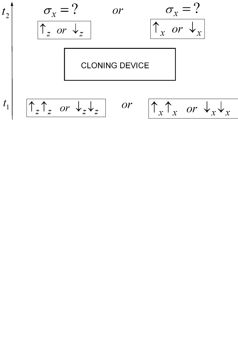
Figure 5: Cloning device for backward evolving quantum state allows sending signals to the past. Decision between measurement of $\sigma_{z}$ or $\sigma_{x}$ at time $t_{2}$ leads to distinguishable mixtures at the earlier time $t_{1}$.

The proof of the no cloning theorem which I have found relies on an argument of causality. (Note the similarity to the history of the discovery of the no cloning theorem NC2 ). It is a contradiction with causality to be able to send signals to the past. Let us assume that we have a black box which performs cloning of quantum states evolving backward in time. We arrange an ensemble of pairs of, spin-$1\over 2$ particles. At time $t$, we measure the spin in the $z$ direction of particles in one half of the ensemble of pairs, and the spin in the $x$ direction of particles in the other half of the ensemble. Then we operate our backward evolving cloning machine which supposedly clones the state of one particle of each pair to the other particle of the pair. Finally, we, in the future, perform either a spin $z$ or a spin $x$ measurement on one particle from each pair. Given that the cloning machine works well, the pairs of the particles will be either in identical spin $z$ states or in identical spin $x$ states. Thus, at time $t$, either all pairs of one half of the ensemble yield the same outcomes, or all pairs of the other half yield the same outcomes, depending on our decision of what to measure at a later time. The cloning machine sends signals to the past. This proves that the cloning machine for backward evolving quantum state does not exist.

VIII Manipulation of the Two-State Vector

We have analyzed what can and what cannot be done for a backward evolving quantum state. It turns out that every manipulation, except “preparation”, which can be performed on the standard, forward evolving quantum state, can be performed on the quantum state evolving backward in time. Moreover, contrary to the case of the quantum state evolving forward in time, it is possible to change the direction of time evolution (together with flipping) of quantum state evolving backward in time. This process can also be combined with teleportation. Given a quantum channel (an entangled pair separated in space) we can teleport and flip the direction of time evolution without sending any classical information. This “teleportation” can be performed to any space-time point, and is not constrained to the forward light cone as the standard teleportation is.

Let us now briefly discuss a quantum system described at a particular time by the two-state vector. It is meaningless to ask whether we can perform a nondemolition measurement on a system described by a two-state vector. Indeed, the vector describing the system should not be changed after the measurement, but there is no such time: for a forward evolving state, “after” means later, whereas for a backward evolving state, “after” means before. It is meaningful to ask whether we can perform a demolition measurement on a system described by a two-state vector. The answer is positive VN , even for composite systems with separated parts.

Next, is it possible to teleport a two-state vector? Although we can teleport both forward evolving and backward evolving quantum states, we cannot teleport the two-state vector. The reason is that the forward evolving state can be teleported only to the future light cone, while the backward evolving state can be teleported only to the backward light cone. Thus, there is no space-time point to which both states can be teleported.

Finally, the answer to the question of whether it is possible to clone a two-state vector is negative, since neither forward evolving nor backward evolving quantum states can be cloned.

It is a pleasure to thank Tamar Ravon for helpful discussions. This work has been supported by the European Commission under the Integrated Project Qubit Applications (QAP) funded by the IST directorate as Contract Number 015848.

References

- (1) Aharonov Y, Bergmann P G, and Lebowitz J L (1964) “Time symmetry in the quantum process of measurement,” Phys. Rev. B 134, 1410-1416.
- (2) Vaidman L (1993) “Lorentz-invariant “elements of reality” and the joint measurability of commuting observables” Phys. Rev. Lett. 70, 3369-3372.
- (3) Vaidman L, Aharonov Y, and Albert D Z (1987) “How to ascertain the values of , , and of a spin- particle” Phys. Rev. Lett. 58, 1385-1387.
- (4) Aharonov Y and Vaidman L (1991) “Complete description of a quantum system at a given time” J. Phys. A 24, 2315-2328.
- (5) Aharonov Y and Vaidman L (1990) “Properties of a quantum system during the time interval between two measurements” Phys. Rev. A 41, 11-20.
- (6) Pegg D T, Barnett S M, Jeffers J (2002) “Quantum retrodiction in open systems” Phys. Rev. A 66, 022106.
- (7) Pearle P (1976) “Reduction of the state vector by a nonlinear Schrodinger equation” Phys. Rev. D13, 857-868.
- (8) Ghirardi G, Rimini A, Weber T (1986)“Unified dynamics for microscopic and macroscopic systems” Phys. Rev. D34, 470-479.
- (9) Albert D, Vaidman L (1989) “On a proposed postulate of state-reduction” Phys. Lett. A 139, 1-4.
- (10) Aicardi F, Borsellino A, Ghirardi GC, Grassi R (1991) “Dynamic models for state-vector reduction - Do they ensure that measurements have outcomes?” Found. Phys. Lett. 4, 109-128.
- (11) Albert D (2000) it Time and Chance, Cambridge, MA: Harvard University Press.
- (12) Vaidman L (2002) “The many-worlds interpretation of quantum mechanics” The Stanford Encyclopedia of Philosophy, Zalta E N (ed.).
- (13) Aharonov Y and Vaidman L (1993) “Measurement of the Schrodinger wave of a single particle” Phys. Lett. A 178, 38-42.
- (14) Vaidman L (1998) “Validity of the Aharonov-Bergmann-Lebowitz rule” Phys. Rev. A 57, 2251-2253.
- (15) Leggett A (1995) “Time’s arrow and the quantum measurement problem” in Time’s Arrows Today, S.F. Savitt, ed. (Cambridge University Press).
- (16) Popescu S and Vaidman L (1994) “Causality constraints on nonlocal quantum measurements” Phys. Rev. A 49, 4331-4338.
- (17) C. H. Bennett et al. (1999) “Quantum nonlocality without entanglement”, Phys. Rev. A 59, 1070-1091.
- (18) Groisman B and Vaidman L (2001) “ Nonlocal variables with product-state eigenstates” J. Phys. A: Math. Gen. 34, 6881-6889.
- (19) Bennett C H, Brassard G, Crepeau C, Jozsa R, Peres A, Wootters W K (1993) “Teleporting an unknown quantum state via dual classical and Einstein-Podolsky-Rosen channels” Phys. Rev. Lett. 70, 1895-1899.
- (20) Vaidman L (2003) “Instantaneous Measurement of Nonlocal Variables” Phys. Rev. Lett. 90, 010402.
- (21) Vaidman L and Nevo I (2006) “Nonlocal Measurements in the Time-Symmetric Quantum Mechanics” Int. J. Mod. Phys. B 20, 1528-1535.
- (22) Wootters W K and Zurek WH (1982) “A single quantum cannot be cloned” Nature 299, 802-803.
- (23) Dieks D (1982) “Communication by EPR devices” Phys. Lett. A 92, 271-272.
- (24) Vaidman L (1994) “Teleportation of quantum states” Phys. Rev. A 49, 1473-1476.