Two-level systems: exact solutions and underlying pseudo-supersymmetry

Abstract

Chains of first-order SUSY transformations for the spin equation are studied in detail. It is shown that the transformation chains are related with a polynomial pseudo-supersymmetry of the system. Simple determinant formulas for the final Hamiltonian of a chain and for solutions of the spin equation are derived. Applications are intended for a two-level atom in an electromagnetic field with a possible time-dependence of the field frequency. For a specific form of this dependence, the time oscillations of the probability to populate the excited level disappear. Under certain conditions this probability becomes a function tending monotonously to a constant value which can exceed $1/2$.

PACS: 03.65.Fd, 11.30.Pb

1 Introduction

It is well-known that complex quantum systems with a discrete energy spectrum (i.e., an atom in an external electric field) can be placed in a special dynamical configuration in which only two stationary states are essential. In those cases the description of a system’s evolution does not require a consideration of the entire Hilbert space. A good approximation is achieved in case the whole Hilbert space is replaced by a two-dimensional linear space. Systems of this kind are called two-level systems, whose evolution is governed by a special system of two differential equations, known as the “spin equation”.

The spin equation arises in many areas of theoretical physics and thus finds a wide range of applications, for instance, the semi-classical theory of laser beams [1], the absorption resonance and nuclear induction experiments [2], the behavior of a molecule in a cavity immersed in electric or magnetic fields [3]. Particularly, we would like to stress the importance of the spin equation in view of its possible applications to quantum computations [4].

The first exact solution of the spin equation was obtained by Rabi [5]. This solution found an extensive physical application in the study of various properties of two-level systems. This fact shows a great importance of exactly solvable models involving the spin equation. In a recent paper [6], some general properties of the spin equation were studied. The authors of [6] give an overview of the known results and obtain new classes of exact solutions to this equation. Among the methods of analysis of exactly solvable spin equations, the method of intertwining operators [7]–[9] plays a special role, since it reveals a new type of symmetry related with two-level systems [8, 9], called the polynomial pseudo-supersymmetry.

In this respect, we would like to remind that the ideas and methods of supersymmetry (SUSY) are recently coming into use in relativistic and nonrelativistic quantum-mechanical problems. Supersymmetric quantum mechanics (SUSY QM), originated from the simplest quantum field model in connection with the problem of a spontaneous SUSY breaking [10], finds more and more extensive applications in theoretical physics (see, e.g., [11]). It was discovered that diverse aspects of SUSY QM are closely related with the method of Darboux transformations, well-known in the soliton theory [12]. Numerous works are devoted to the relation between SUSY QM and the technique of intertwining operators [13, 14].

This article is a continuation of a previous works devoted to the study of exact solutions of two-level systems and the peculiarities related to the corresponding underlying supersymmetry [7]–[9]. Our main objective is to show that a repeated use of simple transformations introduced in the above papers gives rise to a wide range of exactly solvable interactions for the spin equation. It turns out that such a study is convenient in the analysis of equations describing two-level systems written in the form of a one-dimensional stationary Dirac equation with a non-Hermitian Hamiltonian of a special form, in which time plays the role of a spatial variable [7]. In this respect, we can mention that non-Hermitian interaction arises, in particular, in various problems of field theory, statistical mechanics (see, e.g., [15]) and nuclear physics. In connection with the discovery of a large class of complex potentials possessing the so-called $\mathcal{PT}$-symmetry (see, e.g., [16]), which often leads to Hamiltonians with a purely real spectrum, recently an attempt was made once again to construct a complex extension of quantum mechanics [17]. In this respect, it is worth mentioning the paper [18], where the authors show that the use of non-Hermitian (so-called quasi-Hermitian) operators does not contradict the basic principles of quantum mechanics. It should also be noted that such a generalization was not started from scratch, and, in fact, partially goes back to classical works [19].

In this respect, the role of supersymmetry in quantum mechanics may increase [8], since, as was recently shown, SUSY transformations allow one to remove singular points from continuous spectra of non-Hermitian Hamiltonians [20], and to convert non-diagonalizable Hamiltonians into diagonalizable ones [21]. This may enlarge the set of admissible super-Hamiltonians, thus giving an opportunity to extend the theory by new types of interaction.

In [8] it was shown how to construct matrix-differential intertwining operators preserving the special form of a non-Hermitian Dirac Hamiltonian, and in [9] some results were announced related to transformation chains. The technique of simple (first-order in derivatives) intertwining operators adapted to the special case of Rabi oscillations made it possible to discover an interesting physical effect [8]. Namely, as distinct form a constant field frequency when the probability to populate the excited level oscillates with time (Rabi oscillations), there exist such types of time dependence of the field frequency that this probability ceases to oscillate and becomes a monotonously increasing function of time tending to a value which may exceed $1/2$ (in particular, it may be equal to $3/4$ [8]). This property gives the hope that inverse population may be observed in an ensemble of two-level atoms placed in such type of field, and they may exhibit lasing properties. This result was obtained when a single Darboux transformation was applied to a two-level atom.

One of the aims of the present work is a detailed analysis of the above-mentioned transformation chains. In order to make this work self-contained, we show first of all (see the following section) how the Schrödinger equation for a two-level atom interacting in the rotating wave approximation with the electric component of an electromagnetic field can be reduced to a one-dimensional stationary Dirac equation with an effective non-Hermitian Hamiltonian where time plays the role of a spatial variable. This is accomplished for a general time-dependence of the field frequency.

The third section is devoted to supersymmetric constructions. It is shown that the transformation chains introduced in [7, 8] are related with a polynomial pseudo-supersymmetry of the system. This fact indicates the presence of this type of symmetry in a two-level atom.

The introductory part of the fourth section contains a brief review of previous results which are required in the following sections. It is shown that in the case of various factorization constants the use of formulas similar to the Crum–Krein formulas [22] for the Schrödinger equation permits us to express the potential, obtained as a result of an $n$-fold SUSY transformation, through $n$-order determinants of the transformation functions, thus avoiding the use of recurrent formulas, which require the knowledge of solutions at all the intermediary steps. We obtain the form of transformation functions that preserves both the specific matrix structure of the initial potential and its real-valued character. We also study the case of coinciding factorization constants and obtain a sufficiently simple realization of such transformation chains.

As a numerical application of our general scheme, in the final (fifth) section we examine a two-fold transformation for a two-level atom in an external electromagnetic field. We discover that in this case the disappearance of oscillations in the time-dependence of the probability to populate the excited level may also occur, i.e., at certain conditions this probability may acquire a monotonous time-dependence. It is established that, in contrast to the previously published results [8], this effect emerges for two kinds of behavior of the detuning of the external field frequency from the resonance value. In these cases, the probability values to populate the excited level after a two-fold transformation coincide with either the maximal or the minimal values of the probability oscillations obtained as a result of a one-fold transformation.

2 Two-level atom in external field

Since the results obtained in this paper are mainly applied to a two-level atom in an external electromagnetic field, in this section we briefly review some properties of this system which are required in the following sections.

In the non-relativistic approximation, the evolution of a state vector of a two-level atom in an external electromagnetic field with the electric component $\mathbf{E}\left(t\right)=\mathbf{e}E_{0}\cos\left[\omega\left(t\right)t\right]$, where $\mathbf{e}$ is a unit vector of the field polarization, is described by the Schrödinger equation

$$i\hbar\dot{\psi}\left(\mathbf{r},t\right)=\left(H_{0}+H_{1}\right)\psi\left(\mathbf{r},t\right)\,.$$ (1)

Here, $H_{0}$ is the conventional Hamiltonian of an atom in the absence of an external field, $H_{0}\psi_{n}(\mathbf{r})=\varepsilon_{n}\psi_{n}(\mathbf{r})$, $n=1,2;$ $H_{1}$ describes the interaction of the atom with the electric field component in the dipole approximation,

$$H_{1}=\left|q\right|E_{0}\left(\mathbf{e}\cdot\mathbf{r}\right)\cos\left[\omega\left(t\right)t\right]\,;$$

$q<0$ is the charge of electron; the dot over a symbol stands for differentiation with respect to time. We assume that the field frequency, $\omega=\omega\left(t\right)$, and thus also the detuning of the frequency from the resonance value, $\omega_{21}=\omega_{2}-\omega_{1}$,

$$\delta\left(t\right)=\omega(t)-\omega_{21}\,,$$ (2)

are functions of time. Decomposing the solution $\psi\left(\mathbf{r},t\right)$ of equation (1) in the basis $\psi_{n}\left(\mathbf{r}\right)\exp\left(-i\omega_{n}t\right)$, $\omega_{n}=\varepsilon_{n}/\hbar$, $n=1,2,$ we obtain the well-known [23] set of equations for the decomposition coefficients $C_{n}$, $n=1,2$. Introducing the notation $A_{1,2}=\exp\left(\mp i\frac{\delta}{2}t\right)C_{1,2}$ and neglecting the term $\exp\left[i(\omega_{21}+\omega(t))t\right]$, rapidly oscillating in comparison with $\exp\left[i\delta t\right]$ (the so-called rotating wave approximation [23, 24]), we arrive at the following set of equations:

$$i\dot{A}_{1}-fA_{1}=\xi A_{2}\,,\quad i\dot{A}_{2}+fA_{2}=\xi A_{1}\,.$$ (3)

Here, $\xi=\frac{1}{2\hbar}E_{0}d_{21},$

$$f=f(t)=\frac{1}{2}\frac{d}{dt}\left[t\delta(t)\right]\text{\thinspace},$$ (4)

and $d_{21}$ is a matrix element of the dipole momentum operator, $d_{12}=d_{21}=|q|\langle\psi_{1}|\left(\mathbf{e\cdot r}\right)|\psi_{2}\rangle$. If $\omega$ does not depend on time (consequently, $f=\frac{1}{2}\delta=\mathrm{const}$), then solving equations (3) with the initial conditions $A_{2}=0$ and $A_{1}=1$ for $t=0$ we determine the probability to detect the system at the moment $t$ in the excited state on condition that at the initial time moment $t=0$ the system was at the ground state:

$$|A_{2}\left(t\right)|^{2}=\frac{\xi^{2}}{2\Omega^{2}}\left[1-\cos\left(2\Omega t\right)\right],\quad\Omega^{2}=f^{2}+\xi^{2}\,.$$ (5)

This result is well-known in quantum optics [23, 24]. Formula (5) describes the so-called Rabi oscillations, and the value equal to $2\xi$, is known as the Rabi frequency.

Introducing the notation

$$V_{0}(t)=i\sigma_{2}f_{0}\left(t\right),$$ (6)

$\gamma=i\sigma_{1}$, $E=\xi$, $\Psi=\left(A_{1},A_{2}\right)^{\top}$ (the symbol^⊤ stands for transposition, while $\sigma_{1,2,3}$ are the standard Pauli matrices) we rewrite the system of equations (3) at $f=f_{0}$ in the matrix form

$$h_{0}\Psi=E\Psi\,,\quad h_{0}=\gamma\frac{d}{dt}+V_{0}\left(t\right)\,.$$ (7)

Equation (7) has the form of a one-dimensional stationary Dirac system where time plays the role of a spatial variable and $V_{0}\left(t\right)$ is a matrix-valued potential determined by the function $f_{0}\left(t\right)$, which we shall call the potential. Following the well-established terminology, we call $h_{0}$ the Hamiltonian even though in the current case it does not correspond to any quantum-mechanical system. By construction, the parameters $f_{0}$ and $E$ are real.

3 Polynomial pseudo-supersymmetry of a two-level system

Let us assume that the solutions of equation (7) are known and it is necessary to find solutions of this equation with another potential,

$$h_{1}\Phi=E\Phi\,,\quad h_{1}=\gamma\frac{d}{dt}+V_{1}\left(t\right)\,,$$ (8)

where $V_{1}(t)=i\sigma_{2}f_{1}\left(t\right)$. This problem can be solved by finding such an operator $L_{0,1}$ that obeys the following operator equality (intertwining relation):

$$L_{0,1}h_{0}=h_{1}L_{0,1}\,.$$ (9)

In this case, solutions of equation (8) can be found by applying the operator $L_{0,1}$ to solutions of the initial equation (7), $\Phi=L_{0,1}\Psi$.

The intertwining relation (9) provides the basis for the general concept of transformation operators (see, e.g., [25]), and, in particular, operators of Darboux transformations [26]. At the same time, the existence of the intertwining operator $L_{0,1}$ allows one to construct a (generally polynomial) supersymmetry algebra [26] related to equation (7), thus revealing its internal supersymmetric nature.

Usually in optical problems, as distinct from quantum-mechanical problems, the introduction of a Hilbert space is unnecessary. In this case, symmetry operators are defined on the space of solutions of the corresponding equation without introducing any inner product. In the case of a two-level atom, the equation in question is the differential equation (7). For supersymmetric constructions, we shall need the notion of operator conjugation, which will be introduced in a formal way. The operation of formal (Laplace) conjugation obeys the standard rules $(AB)^{{\dagger}}=B^{{\dagger}}A^{{\dagger}}$, $(d/dt)^{{\dagger}}=-d/dt$ and corresponds to the transposition of a matrix accompanied by the complex conjugation of its elements. The operator $A$ is called Hermitian if $A^{{\dagger}}=A$. It is easy to seen from (7) that $h_{0}$ is non-Hermitian. Therefore, along with equation (7) there also exists its adjoint form

$$h_{0}^{{\dagger}}\widetilde{\Psi}=E\widetilde{\Psi}\,.$$ (10)

Another relation that we shall need is obtained by the conjugation of the intertwining relation (9)

$$L_{0,1}^{{\dagger}}h_{1}^{{\dagger}}=h_{0}^{{\dagger}}L_{0,1}^{{\dagger}}\,.$$ (11)

The operator $L_{0,1}$, obviously transforms solutions of equation (7) into solutions of equation (8), while the operator $L_{0,1}^{{\dagger}}$ realizes the backward transformation, i.e., a transformation from solutions of the equation

$$h_{1}^{{\dagger}}\widetilde{\Phi}=E\widetilde{\Phi}\,,\qquad\widetilde{\Phi}=L_{0,1}^{{\dagger}}\widetilde{\Psi}$$

into solutions of equation (10). We shall also assume that the functions $\Psi$, $\widetilde{\Psi}$ and $\Phi$, $\widetilde{\Phi}$, as well as the operators $h_{0}$, $h_{0}^{{\dagger}}$ and $h_{1}$, $h_{1}^{{\dagger}}$ are interrelated by an operator $J$

$$\widetilde{\Psi}=J\Psi\,,\qquad\widetilde{\Phi}=J\Phi\,,$$

which is assumed to have the properties

$$h_{0,1}^{{\dagger}}=Jh_{0,1}J\,,\qquad J^{2}=\pm 1\,,\qquad J^{{\dagger}}=\pm J\,.$$ (12)

From these equations it follows that a superposition of conjugation and the operation $J$ is a pseudo-conjugation, while the operators $h_{0}$ and $h_{1}$ are pseudo-Hermitian [27].

Relations (11) and (12) yield the equality

$$JL_{0,1}^{{\dagger}}Jh_{1}=h_{0}JL_{0,1}^{{\dagger}}J\,.$$

Thus, the operator $JL_{0,1}^{{\dagger}}J$ transforms solutions of the equation with the Hamiltonian $h_{1}$ into solutions corresponding to the Hamiltonian $h_{0},$ while the superposition $JL_{0,1}^{{\dagger}}JL_{0,1}$ transforms solutions of equation (7) into solutions of the same equation, and, therefore, it is a symmetry operator of this equation. In exactly the same manner, the operator $L_{0,1}JL_{0,1}^{{\dagger}}J$ is a symmetry operator of the equation with the Hamiltonian $h_{1}$. Since both these operators are differential, one can expect that the indicated superpositions are polynomials of the corresponding Hamiltonians, a property which we shall demonstrate.

It is easy to see that in the case of Hamiltonian (7) we have $J=\sigma_{x}$. In [8] the authors constructed matrix-differential intertwining operators preserving the specific form (7) of the non-Hermitian Dirac Hamiltonian $h_{0}$ and expressed the symmetry operators $JL_{0,1}^{+}JL_{0,1}$ and $L_{0,1}JL_{0,1}^{+}J$ of equations (7) and (8) in terms of the corresponding Hamiltonians:

$$JL_{0,1}^{+}JL_{0,1}=h_{0}^{2}-\Lambda_{1}^{2}\,,\quad L_{0,1}JL_{0,1}^{+}J=h_{1}^{2}-\Lambda_{1}^{2}\,.$$ (13)

The constant matrix $\Lambda_{1}=\mathrm{diag}(\lambda_{1},-\lambda_{1})$ in (13) is called the (matrix) factorization constant ($\lambda_{1}$ is also called the factorization constant). Formulas (13) present a generalization of the factorization properties of transformation operators that take place in the case of Hermitian one-component Hamiltonians [28].

The presence of a polynomial pseudo-supersymmetry in the system under consideration is related with the possibility of a repeated use of the above one-fold transformation, i.e., with the realization of transformation chains. Let a sequence of transformation operators $L_{0,1}$, $L_{1,2}$, …, $L_{n-1,n}$ intertwines non-Hermitian Hamiltonians $h_{0}$, $h_{1}$, …, $h_{n}$ and all the operators $h_{k}$ have potentials of the form $V_{k}\left(t\right)=i\sigma_{2}f_{k}\left(t\right)$. In this case, every $h_{k}$ has the property

$$h_{k}^{+}=Jh_{k}J\,,\quad k=0,\ldots,n\,.$$ (14)

If we are interested only in the resulting action of the chain, we can introduce the operator $L_{0,n}=L_{n-1,n}\ldots L_{1,2}L_{0,1}$. Due to the intertwining relations which hold for each separate operator $L_{k-1,k}$

$$L_{k-1,k}h_{k-1}=h_{k}L_{k-1,k}\,,\quad k=1,\ldots,n,$$

the operator $L_{0,n}$ obeys the relation

$$L_{0,n}h_{0}=h_{n}L_{0,n}\,.$$ (15)

Conjugating (15) and using (14), we obtain

$$JL_{0,n}^{+}Jh_{n}=h_{0}JL_{0,n}^{+}J\,.$$ (16)

Moreover, for every operator $h_{k}$ there holds the following factorization:

$$JL_{k-1,k}^{+}JL_{k-1,k}=h_{k-1}^{2}-\Lambda_{k}^{2}\,,\quad k=1,\ldots,n$$

with $\Lambda_{k}=\mathrm{diag}(\lambda_{k},-\lambda_{k})$.

Let us consider the superposition

$$JL_{0,n}^{+}JL_{0,n}=JL_{0,1}^{+}L_{1,2}^{+}\ldots L_{n-1,n}^{+}JL_{n-1,n}\ldots L_{1,2}L_{0,1}\,.$$

A subsequent use of separate factorization relations of type (13) and intertwining relations of type (9) yields

$$JL_{0,n}^{+}JL_{0,n}=(h_{0}^{2}-\Lambda_{1}^{2})(h_{0}^{2}-\Lambda_{2}^{2})\ldots(h_{0}^{2}-\Lambda_{n}^{2})\,.$$ (17)

In a similar way, we obtain the factorization of the same polynomial of the operator $h_{n}$

$$L_{0,n}JL_{0,n}^{+}J=(h_{n}^{2}-\Lambda_{1}^{2})(h_{n}^{2}-\Lambda_{2}^{2})\ldots(h_{n}^{2}-\Lambda_{n}^{2})\,.$$ (18)

Let us introduce the following $4\times 4$ matrices:

$$H=\begin{pmatrix}h_{0}&0\\ 0&h_{n}\end{pmatrix}\,,\quad Q_{1}=\begin{pmatrix}0&0\\ L_{0,n}&0\end{pmatrix}\,,\quad Q_{2}=\begin{pmatrix}0&JL_{0,n}^{+}J\\ 0&0\end{pmatrix}.$$

It is easy to see that the intertwining relations (15) and (16) are equivalent to the commutation relations

$$[Q_{1},H]=[Q_{2},H]=0,$$ (19)

while formulas (17) and (18) can be rewritten in the form

$$Q_{1}Q_{2}+Q_{2}Q_{1}=(H^{2}-\Gamma_{1}^{2})(H^{2}-\Gamma_{2}^{2})\ldots(H^{2}-\Gamma_{n}^{2})$$ (20)

where $\Gamma_{k}=\mathrm{diag}(\Lambda_{k},\Lambda_{k})$. It is also obvious that the operators $Q_{1}$ and $Q_{2}$ are nilpotent. Formulas (19) and (20) demonstrate that the operators $H$, $Q_{1}$ and $Q_{2}$ close a polynomial superalgebra thus revealing a hidden polynomial supersymmetry of the system described by the Hamiltonian $h_{0}$. For the first time, superalgebras related with non-Hermitian Hamiltonians were introduced in [27]. From this standpoint, a polynomial pseudo-supersymmetry can be associated with a two-level system.

4 Chains of transformations

4.1 General remarks

Supersymmetric constructions of the previous section are valid if there exist transformation operators $L_{0,1}$,…,$L_{n-1,n}$ preserving the special form (7) of a non-Hermitian Dirac Hamiltonian at each step of transformation where the potential matrix has the form (6). In [8] the authors constructed one-fold matrix-differential intertwining operator $L_{0,1}$ having the necessary properties. In this section, we shall sketch the results of [8] that we shall need in the following sections.

Let us assume that we know $n$ matrix-valued solutions of the equation

$$\left(\gamma\partial_{t}+V_{0}\right)\mathcal{U}_{k}=\mathcal{U}_{k}\Lambda_{k},\quad k=1,\ldots,n\,.$$ (21)

This equation always has a solution,

$$\mathcal{U}_{k}=\left(\begin{array}[]{cc}u_{k}&u_{k}\\ \tilde{u}_{k}&-\tilde{u}_{k}\end{array}\right),$$ (22)

corresponding to the factorization matrix $\Lambda_{k}=\mathrm{diag}\left(iR_{k},-iR_{k}\right)$. The functions $u_{k}$, $\tilde{u}_{k}$ have the same absolute value, and the sum of their phases is a constant, which we denote by $C;$ see eqs. (23), (24)). We choose the matrix-valued function $\mathcal{U}_{1}$ as a transformation function for the first transformation step. The functions $u_{1}$, $\tilde{u}_{1}$ defining the matrix $\mathcal{U}_{1}$ are expressed in terms of a real function $q_{1},$

$$u_{1}=\frac{1-iq_{1}}{\sqrt{1+q_{1}^{2}}}\exp\left[R_{1}\int\frac{1-q_{1}^{2}}{1+q_{1}^{2}}dt\right]e^{i\frac{C}{2}},$$ (23)

$$\tilde{u}_{1}=\frac{1+iq_{1}}{\sqrt{1+q_{1}^{2}}}\exp\left[R_{1}\int\frac{1-q_{1}^{2}}{1+q_{1}^{2}}dt\right]e^{i\frac{C}{2}},$$ (24)

which, in turn, should be found with the help of a real solution $\chi_{1}$ of the second-order equation

$$\ddot{\chi}_{1}+\left[f_{0}^{2}+\frac{1}{2}\frac{d^{2}}{dt^{2}}\left(\ln f_{0}\right)-\left(\frac{\ddot{f}_{0}}{2f_{0}}-R_{1}\right)^{2}\right]\chi_{1}=0$$ (25)

as follows:

$$q_{1}=\frac{R_{1}}{f_{0}}-\frac{\dot{f}_{0}}{2f_{0}^{2}}-\frac{\dot{\chi}_{1}}{f_{0}\chi_{1}}\,.$$ (26)

The transformation operator of the first transformation step $L_{0,1}$ and a new potential $V_{1}$ have the form

$$L_{0,1}=\frac{d}{dt}-W_{1},\quad W_{1}=\dot{\mathcal{U}}_{1}\mathcal{U}_{1}^{-1}\,,$$ (27)

$$V_{1}=V_{0}+\left[\gamma,D_{1}\right],\quad D_{1}=W_{1}\,.$$ (28)

The potential matrix $V_{1}$ (28) has the form (6), where $f_{0}$ should be replaced by $f_{1}$. The function $f_{1}$ and the matrix $W_{1}$ defining the operator $L_{0,1}$ are expressed in terms of the same function $q_{1},$

$$f_{1}=\frac{4R_{1}q_{1}}{1+q_{1}^{2}}-f_{0}\,,$$ (29)

$$W=\mathrm{diag}\left(w_{1},w_{2}\right)\,,\quad w_{1}=-if_{0}+R_{1}\frac{\left(1+iq_{1}\right)^{2}}{1+q_{1}^{2}}\,,\quad w_{2}=w_{1}^{\ast}\,.$$ (30)

If we choose $\lambda_{1}$ to be purely imaginary, the parameter $R_{1}$ becomes real and the differential equation (25) has real coefficients. Due to the fact that an equation with real coefficients always has real solutions, we conclude that for any real-valued function $f_{0}(t)$ one can obtain a real-valued function $f_{1}(t)$ thus realizing a transformation with a real-valued resulting potential.

We now observe that the functions $\mathcal{V}_{k}=L_{0,1}\mathcal{U}_{k}$, $k=2,\ldots,n$ are matrix-valued solutions of equation (21) with potential (28). At the next step of transformation, we choose $\mathcal{V}_{2}$ as a transformation function, thus obtaining the operator $L_{1,2}$ and potential $V_{2}$

$$L_{1,2}=\frac{d}{dt}-W_{2},\quad W_{2}=\dot{\mathcal{V}}_{2}\mathcal{V}_{2}^{-1}\,,$$ (31)

$$V_{2}=V_{1}+\left[\gamma,W_{2}\right]=V_{0}+\left[\gamma,D_{2}\right],\quad D_{2}=D_{1}+W_{2}\,.$$

The operator $L_{0,2}=L_{1,2}L_{0,1}$ is a differential operator of second order with matrix-valued coefficients, intertwining the Hamiltonians $h_{0}$ and $h_{2}=\gamma\partial_{t}+V_{2}$, $L_{0,2}h_{0}=h_{2}L_{0,2}$.

Continuing this process, one can construct the $n$-th order operator

$$L_{0,n}=L_{n-1,n}\ldots L_{1,2}L_{0,1}\,,$$ (32)

which transforms the Hamiltonian $h_{0}$ into the Hamiltonian $h_{n}$ with the potential

$$V_{n}=V_{n-1}+[\gamma,W_{n}]=V_{0}+\left[\gamma,D_{n}\right],\quad D_{n}=D_{n-1}+W_{n}\,,\quad D_{0}=0\,,$$ (33)

where

$$W_{n}=\dot{\mathcal{Y}}_{n}\mathcal{Y}_{n}^{-1},\quad\mathcal{Y}_{n}=L_{0,n-1}\mathcal{U}_{n}\,.$$ (34)

The derivation of the transformed potential $V_{n}$ by the recurrent formulas (33) and (34) involves a calculation of all the intermediary potentials and transformation functions, which requires a large amount of computational work. Below, we will show how to overcome this difficulty in the case when all the factorization constants $R_{1}$, …, $R_{n}$ are different from each other. For coinciding factorization constants, we will show that equation (25) may be solved in quadratures for any initial potential $f_{0}$ which also yields an essential simplification of the method.

4.2 Transformations with coinciding factorization constants

Let us consider a chain of two transformations. In order to obtain the potential $f_{2},$ we have to make the replacement $R_{1}\rightarrow R_{2}$, $q_{1}\rightarrow q_{2}$, $f_{1}\rightarrow f_{2}$, $f_{0}\rightarrow f_{1}$ in (29), and then $f_{1}$ in the obtained equation should be substituted by using the same equation (29). This yields

$$f_{2}=f_{0}-\frac{4R_{1}q_{1}}{1+q_{1}^{2}}+\frac{4R_{2}q_{2}}{1+q_{2}^{2}}\;.$$ (35)

In (35) the function $q_{2}$ is expressed through the solution $\chi_{2}$ of equation (25) with $f_{0}=f_{1}$ and $R_{1}=R_{2}$ by formula (26), where the necessary replacements should be made. A generalization of this procedure to the case of a chain of $n$ transformations is obvious. However, the form of both the potential and solutions to equation (25) after each transformation step will become more and more complicated. It is remarkable that, in case the transformation chain is realized by coinciding factorization constants, equation (25) can be integrated explicitly. This makes it possible to get rid of this equation and express the new potential $f_{2}$ in terms of the potential $f_{1}$ alone.

Note, first of all, that according to (35), for $R_{1}=R_{2}$ and $q_{2}=q_{1}$ or $q_{2}=q_{1}^{-1},$ the potential $f_{2}$ assumes the value of the initial potential $f_{0}$, i.e., the second transformation step is equivalent to a reverse transformation. The case $q_{2}=q_{1}$ corresponds to a trivial transformation, for which all of the three potentials remain the same, $f_{2}=f_{1}=f_{0}$, whereas for $q_{2}=q_{1}^{-1}$ one obtains a nontrivial result. Therefore, for $R_{2}=R_{1}$ the inverse transformation corresponds to $q_{2}=q_{1}^{-1}$. Then using formula (26) for $q_{2},$ in which we have to put $q_{1}=q_{2}$, $f_{0}=f_{1}$, $\chi_{1}=\chi_{2},$ we obtain the following differential equation with respect to the function $\chi_{2}$:

$$q_{1}^{-1}=\frac{R_{1}}{f_{1}}-\frac{\dot{f}_{1}}{2f_{1}^{2}}-\frac{\dot{\chi}_{2}}{f_{1}\chi_{2}}$$ (36)

which can be easily integrated:

$$\chi_{2}=\tilde{C}\exp\int\left(R_{1}-\frac{\dot{f}_{1}}{2f_{1}}-\frac{f_{1}}{q_{1}}\right)dt\,.$$ (37)

Here, $\tilde{C}$ is an integration constant. Equation (25) with fixed values of $f_{0}$ and $R_{1},$ being a second-order differential equation, has two linearly independent solutions. Using the fact that the Wronskian of any two linearly independent solutions to equation (25) is constant [29], we can obtain a solution of this equation, which is linearly independent from (37). This permits us to find the potential $f_{2}$ different from $f_{0}$, i.e., to accomplish the second nontrivial step of transformation, with the same value of the factorization constant. To this end, let us define the function $\tilde{\chi_{2}}$ as the second solution of equation (25) satisfying the condition $W\left(\chi_{2},\tilde{\chi}_{2}\right)=1,$ where $W$ denotes the Wronskian. Then the function $\tilde{\chi}_{2}$ is expressed in terms of ${\chi}_{2}$ as follows:

$$\tilde{\chi}_{2}=\chi_{2}\int\chi_{2}^{-2}dt\,.$$ (38)

Thus, in order to obtain a real potential by a two-fold transformation with coinciding factorization constants, it is now unnecessary to solve equation (25) at the second step of transformation, since the structure of its solution leading to a nontrivial result is determined and expressed in terms of quantities known as a result of the first transformation step.

Let us express the result of consecutive application of transformations with coinciding factorization constants in the general form. A solution of equation (25) subject to the substitution $f_{0}\rightarrow f_{n-1}$ and $R_{1}\rightarrow R_{n}$ corresponding to the inverse transformation such that $f_{n}=f_{n-2}$ has the form

$$\chi_{n}=\tilde{C}\exp\int\left(R_{n-1}-\frac{\dot{f}_{n-1}}{2f_{n-1}}-\frac{f_{n-1}}{q_{n-1}}\right)dt\,,$$ (39)

where $R_{n}=R_{n-1}$. By analogy with (38), we obtain the second solution $\tilde{\chi}_{n}$ of this equation linearly independent from (39), corresponding to another nontrivial step of a many-fold transformation. The new potential can be found by formula (29) subject to the substitution $f_{0}\rightarrow f_{n-1}$ and $q_{1}\rightarrow q_{n}$, where

$$q_{n}=\frac{R_{n}}{f_{n-1}}-\frac{\dot{f}_{n-1}}{2f_{n-1}^{2}}-\frac{\dot{\tilde{\chi_{n}}}}{f_{n-1}\tilde{\chi}_{n}}\,.$$ (40)

Thus, the use of transformation chains with coinciding factorization constants allows one to easily obtain new exactly solvable potentials.

4.3 Transformations with different factorization constants

As we have already mentioned, the explicit solution of equation (25) becomes problematic in the case of a many-fold transformation. The integration of this equation can be avoided by using formulas similar to the Crum–Krein formulas [22], well-known for the Schrödinger equation, which allow one to express the potential after an $n$-fold transformation in terms of determinants of transformation functions. This question was considered in detail for a matrix Schrödinger equation [30] and a Dirac equation [14] with Hermitian Hamiltonians. Below, we will investigate the peculiarities arising during the use of these formulas for the Dirac equation (7) with the effective non-Hermitian Hamiltonian $h_{0}$ and transformation functions of a special type, which do not change the form of a Hamiltonian after a transformation and obey conditions necessary for the transformed potential to remain a real value.

We start by reminding some results concerning chains of transformations for the Dirac equation obtained in [14, 30]. According to these articles, the entries $d_{ij}^{n}$, $i,j=1,2$ of the matrix $D_{n}$ in (33) are expressed in terms of the transformation functions $\mathcal{U}_{k}$, $k=1,\ldots,n$ as follows:

$$d_{ij}^{n}=\frac{|P_{ij}\left(\mathcal{U}_{1},\ldots,\mathcal{U}_{n}\right)|}{|P\left(\mathcal{U}_{1},\ldots,\mathcal{U}_{n}\right)|}\,.$$

Here, $P\left(\mathcal{U}_{1},\ldots,\mathcal{U}_{n}\right)$ is the Wronsky matrix constructed from the matrix-valued functions $\mathcal{U}_{k}$, $k=1,\ldots,n$,

$$P\left(\mathcal{U}_{1},\ldots,\mathcal{U}_{n}\right)=\left(\begin{array}[]{cccc}\mathcal{U}_{1}&\mathcal{U}_{2}&\ldots&\mathcal{U}_{n}\\ \mathcal{U}_{1}{}^{\prime}&\mathcal{U}_{2}{}^{\prime}&\ldots&\mathcal{U}_{n}{}^{\prime}\\ \ldots&\ldots&\ldots&\ldots\\ \mathcal{U}_{1}^{\left(n-1\right)}&\mathcal{U}_{2}^{\left(n-1\right)}&\ldots&\mathcal{U}_{n}^{\left(n-1\right)}\end{array}\right);$$ (41)

the matrix $P_{ij}\left(\mathcal{U}_{1},\ldots,\mathcal{U}_{n}\right)$ has a structure similar to that of $P\left(\mathcal{U}_{1},\ldots,\mathcal{U}_{n}\right)$ with the exception that the final row consisting of matrices $\mathcal{U}_{k}^{\left(n-1\right)}$ is replaced by matrices $\mathcal{U}_{k}^{ij}$, $k=1,\ldots,n$:

$$P_{ij}\left(\mathcal{U}_{1},\ldots,\mathcal{U}_{n}\right)=\left(\begin{array}[]{cccc}\mathcal{U}_{1}&\mathcal{U}_{2}&\ldots&\mathcal{U}_{n}\\ \mathcal{U}_{1}{}^{\prime}&\mathcal{U}_{2}{}^{\prime}&\ldots&\mathcal{U}_{n}{}^{\prime}\\ \ldots&\ldots&\ldots&\ldots\\ \mathcal{U}_{1}^{\left(n-2\right)}&\mathcal{U}_{2}^{\left(n-2\right)}&\ldots&\mathcal{U}_{n}^{\left(n-2\right)}\\ \mathcal{U}_{1}^{ij}&\mathcal{U}_{2}^{ij}&\ldots&\mathcal{U}_{n}^{ij}\end{array}\right).$$

The matrices $\mathcal{U}_{k}^{ij}$, $i,j=1,2$ follow from $\mathcal{U}_{k}^{\left(n-1\right)}$ by the replacement of the $j$-th row by the $i$-th row of the matrix $\mathcal{U}_{k}^{\left(n\right)}$.

In [30] it was shown that the action of the operator $L_{0,n}$ (32) on the function $\Psi_{E}=\left(\psi_{1E},\psi_{2E}\right)^{\top}$ yields a vector $\Phi_{E}=\left(\phi_{1E},\phi_{2E}\right)^{\top}$ with the entries

$$\phi_{jE}=\frac{|P_{jE}\left(\mathcal{U}_{1},\ldots,\mathcal{U}_{n}\right)|}{|P\left(\mathcal{U}_{1},\ldots,\mathcal{U}_{n}\right)|}\;,\quad j=1,2\;.$$ (42)

In (42) the matrix $P_{jE}\left(\mathcal{U}_{1},\ldots,\mathcal{U}_{n}\right)$ has the form

$$P_{jE}\left(\mathcal{U}_{1},\ldots,\mathcal{U}_{n}\right)=\left(\begin{array}[]{ccccc}\mathcal{U}_{1}&\mathcal{U}_{2}&\ldots&\mathcal{U}_{n}&\Psi_{E}\\ \mathcal{U}_{1}{}^{\prime}&\mathcal{U}_{2}{}^{\prime}&\ldots&\mathcal{U}_{n}{}^{\prime}&\Psi_{E}^{\prime}\\ \ldots&\ldots&\ldots&\ldots&\ldots\\ \mathcal{U}_{1}^{\left(n-1\right)}&\mathcal{U}_{2}^{\left(n-1\right)}&\ldots&\mathcal{U}_{n}^{\left(n-1\right)}&\Psi_{E}^{\left(n-1\right)}\\ \left(\mathcal{U}_{1}^{j}\right)^{\left(n\right)}&\left(\mathcal{U}_{2}^{j}\right)^{\left(n\right)}&\ldots&\left(\mathcal{U}_{n}^{j}\right)^{\left(n\right)}&\psi_{jE}^{\left(n\right)}\end{array}\right),$$ (43)

where $\mathcal{U}_{k}^{j}$ is the $j$-th row of the matrix $\mathcal{U}_{k}$. These formulas are obtained as a closure of the recursion scheme defined by equations (33) and (34). This algorithm will preserve the particular form of potential (6) provided that the transformation operators $L_{k-1,k}$ preserve the form (22) of the transformation function at every transformation step, a property which we will now demonstrate by induction.

Let the transformation function $\mathcal{U}_{1}$ of the first transformation step have the required form (22). We also assume that this property takes place at the $(k-1)$-st transformation step:

$$\mathcal{V}_{j}=L_{0,k-2}\mathcal{U}_{j}=\left(\begin{array}[]{cc}v_{j}&v_{j}\\ \tilde{v}_{j}&-\tilde{v}_{j}\end{array}\right),\quad j=k-1,k,\ldots,n\,.$$ (44)

Then the transformation function at the $k$-th step is expressed as follows:

$$\mathcal{Y}_{k}=L_{k-2,k-1}\mathcal{V}_{k},\quad L_{k-2,k-1}=\left(\frac{d}{dt}-\dot{\mathcal{V}}_{k-1}\mathcal{V}_{k-1}^{-1}\right).$$ (45)

Using (44), we find, just as we expected, that (45) implies

$$\mathcal{Y}_{k}=\left(\begin{array}[]{cc}\mathrm{y}_{k}&\mathrm{y}_{k}\\ \mathrm{\tilde{y}}_{k}&-\mathrm{\tilde{y}}_{k}\end{array}\right),\quad\mathrm{y}_{k}=\dot{v}_{k}-\frac{\dot{v}_{k-1}}{v_{k-1}}\,v_{k}\,.$$

It has been noted that for a purely imaginary parameters $\Lambda_{k}$ the condition necessary for the transformed potential to be a real value is the condition that the absolute values of the elements of the matrix-valued transformation function $\mathcal{U}$ be equal. One can see that the set of functions (22) actually meets this condition. Therefore, these functions allow one to realize a transformation chain which preserves both the special form of the potential and the condition for the function $f_{k}$ to be real-valued.

We are now going to show that for the choice of transformation functions in the form (22) the matrices of $(2n)$-th order $P\left(\mathcal{U}_{1},\ldots,\mathcal{U}_{n}\right)$, $P_{ij}\left(\mathcal{U}_{1},\ldots,\mathcal{U}_{n}\right)$ assume a block form with one of the blocks being a zero matrix. As a result, the determinants $|P\left(\mathcal{U}_{1},\ldots,\mathcal{U}_{n}\right)|$, $|P_{ij}\left(\mathcal{U}_{1},\ldots,\mathcal{U}_{n}\right)|$ are reduced to the product of two determinants of $n$-th order. Let us consider in more detail how this happens for $n=2$, and then present the result for an arbitrary $n$.

In what follows, the elements, rows and columns of a determinant are understood as the elements, rows and columns of the corresponding matrix.

According to (41), the determinant $|P\left(\mathcal{U}_{1},\ldots,\mathcal{U}_{n}\right)|$ for $n=2$ has the form:

$$|P\left(\mathcal{U}_{1},\mathcal{U}_{2}\right)|=\begin{vmatrix}u_{1}&u_{1}&u_{2}&u_{2}\\ \tilde{u}_{1}&-\tilde{u}_{1}&\tilde{u}_{2}&-\tilde{u}_{2}\\ u_{1}^{\prime}&u_{1}^{\prime}&u_{2}^{\prime}&u_{2}^{\prime}\\ {\tilde{u}_{1}}^{\prime}&{-\tilde{u}_{1}}^{\prime}&{\tilde{u}_{2}}^{\prime}&{-\tilde{u}_{2}}^{\prime}\end{vmatrix}.$$ (46)

Subtracting from the second column the first one, and from the forth column the third one, and transmuting the rows and columns, we reduce the determinant (46) to the product of two second-order determinants:

$$|P\left(\mathcal{U}_{1},\mathcal{U}_{2}\right)|=\begin{vmatrix}u_{1}&u_{2}&0&0\\ u_{1}^{\prime}&u_{2}^{\prime}&0&0\\ \tilde{u}_{1}&\tilde{u}_{2}&-2\tilde{u}_{1}&-2\tilde{u}_{2}\\ {\tilde{u}_{1}}^{\prime}&{\tilde{u}_{2}}^{\prime}&{-2\tilde{u}_{1}}^{\prime}&{-2\tilde{u}_{2}}^{\prime}\end{vmatrix}=\begin{vmatrix}u_{1}&u_{2}\\ u_{1}^{\prime}&u_{2}^{\prime}\end{vmatrix}\left(-2\right)^{2}\begin{vmatrix}\tilde{u}_{1}&\tilde{u}_{2}\\ {\tilde{u}_{1}}^{\prime}&{\tilde{u}_{2}}^{\prime}\end{vmatrix}.$$

It is clear that in general we have $|P\left(\mathcal{U}_{1},\ldots,\mathcal{U}_{n}\right)|=\left(-2\right)^{n}p_{1}p_{2}$, where

$$p_{1}=\begin{vmatrix}u_{1}&u_{2}&\ldots&u_{n}\\ u_{1}^{\prime}&u_{2}^{\prime}&\ldots&u_{n}^{\prime}\\ \ldots&\ldots&\ldots&\ldots\\ u_{1}^{\left(n-2\right)}&u_{2}^{\left(n-2\right)}&\ldots&u_{n}^{\left(n-2\right)}\\ u_{1}^{\left(n-1\right)}&u_{2}^{\left(n-1\right)}&\ldots&u_{n}^{\left(n-1\right)}\end{vmatrix},\quad p_{2}=\begin{vmatrix}\tilde{u}_{1}&\tilde{u}_{2}&\ldots&\tilde{u}_{n}\\ \tilde{u}_{1}^{\prime}&\tilde{u}_{2}^{\prime}&\ldots&\tilde{u}_{n}^{\prime}\\ \ldots&\ldots&\ldots&\ldots\\ \tilde{u}_{1}^{\left(n-2\right)}&\tilde{u}_{2}^{\left(n-2\right)}&\ldots&\tilde{u}_{n}^{\left(n-2\right)}\\ \tilde{u}_{1}^{\left(n-1\right)}&\tilde{u}_{2}^{\left(n-1\right)}&\ldots&\tilde{u}_{n}^{\left(n-1\right)}\end{vmatrix}.$$

Similar calculations allow one to simplify the determinants of the matrices $P_{11}\left(\mathcal{U}_{1},\ldots,\mathcal{U}_{n}\right)$ and $P_{22}\left(\mathcal{U}_{1},\ldots,\mathcal{U}_{n}\right)$:

$$|P_{11}\left(\mathcal{U}_{1},\ldots,\mathcal{U}_{n}\right)|=\left(-2\right)^{n}r_{1}p_{2}\,,\quad|P_{22}\left(\mathcal{U}_{1},\ldots,\mathcal{U}_{n}\right)|=\left(-2\right)^{n}p_{1}r_{2}\,,$$

where

$$r_{1}=\begin{vmatrix}u_{1}&u_{2}&\ldots&u_{n}\\ u_{1}^{\prime}&u_{2}^{\prime}&\ldots&u_{n}^{\prime}\\ \ldots&\ldots&\ldots&\ldots\\ u_{1}^{\left(n-2\right)}&u_{2}^{\left(n-2\right)}&\ldots&u_{n}^{\left(n-2\right)}\\ u_{1}^{\left(n\right)}&u_{2}^{\left(n\right)}&\ldots&u_{n}^{\left(n\right)}\end{vmatrix},\quad r_{2}=\begin{vmatrix}\tilde{u}_{1}&\tilde{u}_{2}&\ldots&\tilde{u}_{n}\\ \tilde{u}_{1}^{\prime}&\tilde{u}_{2}^{\prime}&\ldots&\tilde{u}_{n}^{\prime}\\ \ldots&\ldots&\ldots&\ldots\\ \tilde{u}_{1}^{\left(n-2\right)}&\tilde{u}_{2}^{\left(n-2\right)}&\ldots&\tilde{u}_{n}^{\left(n-2\right)}\\ \tilde{u}_{1}^{\left(n\right)}&\tilde{u}_{2}^{\left(n\right)}&\ldots&\tilde{u}_{n}^{\left(n\right)}\end{vmatrix}\,.$$

The determinants of the matrices $P_{12}\left(\mathcal{U}_{1},\ldots,\mathcal{U}_{n}\right)$ and $P_{21}\left(\mathcal{U}_{1},\ldots,\mathcal{U}_{n}\right)$ for the transformation functions (22) are equal to zero. Threfore, the matrix $D_{n}$ from (33) becomes $D_{n}=\mathrm{diag}\left(\frac{r_{1}}{p_{1}},\frac{r_{2}}{p_{2}}\right)$ and $V_{n}$ can be written in the form

$$V_{n}=V_{0}+\Delta V_{n},\quad\Delta V_{n}=i\sigma_{2}\Delta f_{n},\quad\Delta f_{n}=f_{n}-f_{0}=-i\left[\frac{r_{1}}{p_{1}}-\frac{r_{2}}{p_{2}}\right].$$

Thus, we have shown that the use of the determinant technique for an $n$-fold transformation of the spin equation, which is similar to the Crum–Krein approach to the Schrödinger equation, permits us to reduce the method to calculating only $n$-th order determinants.

5 Transformations of the Rabi oscillations

The Rabi oscillations occur at $f_{0}=\mathrm{const}$. In [8] a detailed analysis of solutions to the set of equations (7) constructed with the help of a one-fold transformation is given. Here, we shall study the effect of a two-fold transformation.

Let us first consider the probability to populate the excited level obtained as a result of a two-fold transformation with coinciding factorization constants $R_{2}=R_{1}$. For $f_{0}=\mathrm{const}$, equation (25) takes a very simple form:

$$\ddot{\chi_{1}}+\varpi^{2}\chi_{1}=0\,,\quad\varpi^{2}=f_{0}^{2}-R_{1}^{2}.$$ (47)

Solutions of this equation have various properties depending on whether the value of $\varpi^{2}$ is positive, negative or zero. We have found [8] that the Rabi oscillations after a one-fold transformation disappear for $\varpi=0$. In this case, the general solution of equation (47) is a linear function of time, $\chi_{1}=At+B$, which in the case $A=2Bf_{0}$ yields the following expression for the function $q_{1}$: $q_{1}=1-2/\left(2f_{0}t+1\right)$. The potential after the one-fold transformation reads

$$f_{1}(t)=f_{0}-\frac{4f_{0}}{1+4f_{0}^{2}t^{2}}\,.$$

Let us make the next transformation with $R_{2}=R_{1}$. The function $q_{2}$ is found from (40) at $n=2$, where $\widetilde{\chi}_{2}$ is determined by formulas (37)-(38). Using (35), we get the following expression for the transformed potential:

$$f_{2}\left(t\right)=\frac{f_{0}(-648(-1+4f_{0}^{2}t^{2})-243(1+4f_{0}^{2}t^{2})^{2}+(C-6f_{0}t(9+4f_{0}^{2}t^{2}))^{2})}{81(1+4f_{0}^{2}t^{2})^{2}+(C-6f_{0}t(-3+4f_{0}^{2}t^{2}))^{2}}\,,$$ (48)

where $C$ is a constant.

Let us determine the form of the external electric field $E=E(t)=E_{0}\cos\left[t\omega_{2}\left(t\right)\right]$ corresponding to the potential $f_{2}\left(t\right)$ (48). We may observe an interesting feature of the behavior of $E(t)$ with time. From (2) and (4), it follows that the frequency $\omega_{2}\left(t\right)$ is expressed through the function $f_{2}\left(t\right)$ as follows:

$$\omega_{2}\left(t\right)=\omega_{21}+\delta_{2}\left(t\right),\quad\delta_{2}\left(t\right)=\frac{2}{t}\int_{0}^{t}f_{2}\left(\tau\right)d\tau\,.$$ (49)

In general, the field $E(t)$ is an oscillating function with the amplitude $E_{0}$ (see Fig. 1) except for a special time dependence of $\delta_{2}(t)$. In particular, it may happen that $\delta_{2}(t)$, as found from (49), is expressed in terms of an inverse trigonometric function shifted by a constant $c_{0}$. If $c_{0}+\omega_{21}=0$, the function $\cos[t\omega_{2}(t)]$ may become polynomial. For instance, substituting in (48) $C=0$ and $f_{0}=-1,$ we obtain for $\omega_{2}(t)$

$$\omega_{2}(t)=\omega_{21}-2+\frac{4}{t}\arctan\left(\frac{8t^{3}-6t}{12t^{2}+3}\right)\,.$$

Thus, for $\omega_{21}=2$ the field $E$ becomes the polynomial

$$E(t)=E_{0}\left(1-\frac{5184(1+16t^{2}+48t^{4})}{(9+108t^{2}+48t^{4}+64t^{6})^{2}}+\frac{288(2+7t^{2}-4t^{4})}{9+108t^{2}+48t^{4}+64t^{6}}\right)$$

plotted in Fig.2.

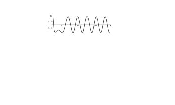
Figure 1: The electric component of the external electromagnetic field $f_{0}=1$, $C=0$, $w_{21}=1$, $E_{0}=0.5$.

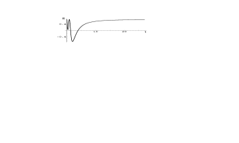
Figure 2: The electric component of the external electromagnetic field after a two-fold transformation with the parameter values $f_{0}=-1$, $C=0$, $w_{21}=2$, $E_{0}=0.7$.

Another interesting effect has been observed for a one-fold transformation [8]. It consists in the disappearance of oscillations in the time-dependence of the excited level population. For a two-fold transformation, there are additional possibilities for observing this property.

Solutions of the initial problem for $f=f_{1}$ are known [8]. Having constructed the transformation operator by using (27) and (31), we find the solutions $A_{12}(t)$ and $A_{22}(t)$ of the set of equations after the second step of transformation. Note that the normalization of solutions changes as a result of the transformation $A_{12}^{2}+A_{22}^{2}=\left(\xi^{2}+R_{1}^{2}\right)^{2}$. Imposing on the solutions the initial conditions $A_{12}(0)=1$ and $A_{22}(0)=0,$ we determine the probability to populate the excited level after a two-fold transformation. The expression for the probability is rather involved and we will not present it here. We merely note that this quantity oscillates with time due to the presence of trigonometric functions.

Let us consider the case $C=0$ in more detail. It turns out that under the condition

$$5f_{0}^{4}-10f_{0}^{2}\xi^{2}+\xi^{4}=0,$$ (50)

the oscillations in the time dependence of the probability disappear and it acquires a monotonous character:

$$P_{2}\left(t\right)=|A_{22}|^{2}=$$

$$\frac{2000t^{2}\xi^{2}(45(25+11\sqrt{5})+60(123+55\sqrt{5})t^{2}\xi^{2}+32(1525+682\sqrt{5})t^{4}\xi^{4})}{(5+\sqrt{5})^{5}(225+540(5+2\sqrt{5})t^{2}\xi^{2}+240(9+4\sqrt{5})t^{4}\xi^{4}+64(85+38\sqrt{5})t^{6}\xi^{6})}\,.$$

Therefore, according to (50), as distinct from one-fold transformations, for two-fold transformations we can indicate two possibilities, $f_{0}^{2}=\xi^{2}\left(1+\frac{2}{\sqrt{5}}\right)$ and $f_{0}^{2}=\xi^{2}\left(1-\frac{2}{\sqrt{5}}\right)$, which transform the probability to populate the excited level from an oscillating function of time to a monotonous one. The plots of probability in these cases are given by Figs. 3 and 4 (thick lines).

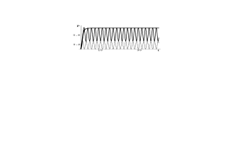
Figure 3: The probability of population of the excited level before the transformation, and after the first and second transformations for $f_{0}^{2}=\xi^{2}\left(1+\frac{2\sqrt{5}}{5}\right)$, $\xi=1$.

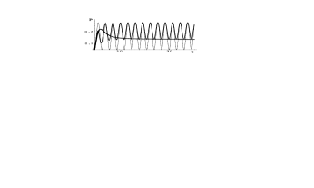
Figure 4: The probability of population of the excited level before the transformation, and after the first and second transformations for $f_{0}^{2}=\xi^{2}\left(1-\frac{2\sqrt{5}}{5}\right)$, $\xi=1$.

We observe another interesting effect by plotting simultaneously the probability to populate the excited level before the transformation and after the first and second transformation steps. Fig. 5 presents the probability plots for a particular value of the parameter $f_{0}^{2}=\frac{1}{3}\xi^{2}$, which corresponds to the case when the probability of population resulting from the one-fold transformation is described by a monotonous function [8]

$$P_{1}(t)=|A_{12}|^{2}=\frac{3f_{0}^{2}t^{2}}{1+4f_{0}^{2}t^{2}}\,.$$ (51)

The thick line presents the plot of probability (51). Its maximal value coincides with the probability before the transformation, i.e., with the probability for the usual Rabi oscillations (the dotted line). The thin line presents the probability resulting from a chain of two transformations. We see from Fig. 5 that the oscillations in this case are in antiphase with the Rabi oscillations.

Figure 5: The probability of population of the excited level before the transformation, and after the first and second transformations for $f_{0}^{2}=\frac{1}{3}\xi^{2}$, $\xi=1$.

Returning to Figs. 3 and 4, note that they also present the plots for $f_{0}^{2}=\xi^{2}\left(1+\frac{2}{\sqrt{5}}\right)$ and $f_{0}^{2}=\xi^{2}\left(1-\frac{2}{\sqrt{5}}\right)$, respectively. For such values of $f_{0},$ the probability to populate the excited level after the two-fold transformation becomes a monotonous function and for $t\rightarrow\infty$ the probability values after the second transformation (the thick line) coincide with either the maxima or the minima of probability oscillations resulting from the one-fold transformation (the thin line). The probability before the transformation (the dotted line) oscillates in this case in phase with the probability after the one-fold transformation.

Omitting the details, let us consider the behavior of the probability to populate the excited level obtained as a result of a two-fold transformation with different factorization constants. The transformed potential $f_{2}$ is obtained in [9]

$$f_{2}=f_{0}-i\left(R_{2}^{2}-R_{1}^{2}\right)\frac{R_{2}\left[B_{2}^{2}-\left(B_{2}^{\ast}\right)^{2}\right]-R_{1}\left[B_{1}^{2}-\left(B_{1}^{\ast}\right)^{2}\right]}{|R_{2}B_{2}-R_{1}B_{1}|^{2}}\;,$$

$$B_{k}=\frac{u_{k}}{\tilde{u}_{k}}=\frac{1-iq_{k}}{1+iq_{k}}\;,\quad k=1,2\,.$$ (52)

Using (42) and (43), we construct the intertwining operator $L_{02}$ and then apply it to find solutions $A_{12}\left(t\right)$ and $A_{22}\left(t\right)$ of equation (7) with potential (52). In terms of the functions $B_{k},$ the operator $L_{02}$ is written as

$$L_{02}=\frac{d^{2}}{dt^{2}}+S_{1}\frac{d}{dt}+S_{2}\,,$$

where

$$S_{1}=\left(\begin{array}[]{cc}s_{1}&0\\ 0&s_{1}^{\ast}\end{array}\right),\quad s_{1}=\frac{R_{1}^{2}-R_{2}^{2}}{R_{2}B_{2}^{\ast}-R_{1}B_{1}^{\ast}}\,,$$

$$S_{2}=\left(\begin{array}[]{cc}s_{2}&0\\ 0&s_{2}^{\ast}\end{array}\right),\quad s_{2}=if_{0}^{\prime}+f_{0}^{2}+\frac{R_{1}R_{2}\left(R_{2}B_{1}^{\ast}-R_{1}B_{2}^{\ast}\right)-if_{0}\left(R_{2}^{2}-R_{1}^{2}\right)}{R_{2}B_{2}^{\ast}-R_{1}B_{1}^{\ast}}\,.$$

Let

$$q_{k}\left(t\right)=\frac{R_{k}\cos\varpi_{k}t+\frac{1}{2}\varpi_{k}\sin\varpi_{k}t-f_{0}}{f_{0}\cos\varpi_{k}t-R_{k}},\;\varpi_{k}=2\sqrt{f_{0}^{2}-R_{k}^{2}},\;k=1,2.$$

Acting by $L_{02}$ on solutions of the initial problem (7), we obtain its solutions for $f_{0}=f_{2}$. Imposing on these solutions the initial conditions $A_{12}\left(0\right)=1$ and $A_{22}\left(0\right)=0$, we determine the probability to populate the excited level after a two-fold transformation. In general, the behavior of probability has an oscillating character. It is important to note that we now observe two kinds of oscillations: small-amplitude and large-frequency (fast) oscillations occur at the background of a large amplitude and small frequency (slow) oscillations (see Fig. 6). Furthermore, at certain values of parameters, the probability for fast oscillations changes within a narrow range (on Fig. 6 between $0.8$ and $0.95$) with the maximal value close to unity.

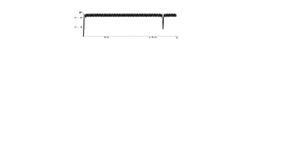
Figure 6: The probability of population of the excited level as a result of a two-fold transformation for different factorization constants: $f_{0}=1$, $R_{1}=0.993$, $R_{2}=0.995$, $\xi=0.65$.

This behavior of probability continues for a long time (on Fig. 6 for approximately $170$ time units that we use). However, the time during which the probability of a transition to an exited state is less than $0.5$ (in the present case it approximately is equal to $0.35$) is less than the indicated interval by several orders of units (approximately two units in the current case). This means that in the course of time the most part of two-level atoms are found in the excited state, which may lead to the appearance of an inverse population, as well as to a possible appearance of the lasing property of an ensemble of two-level atoms placed in such kind of field.

6 Conclusion

We have considered chains of SUSY transformations for the spin equation, with an application to a two-level atom in an external electromagnetic field with a possible time-dependence of the field frequency. It is shown that when a chain of $n$ transformations is replaced by a single $n$-fold transformation one can construct a super-Hamiltonian and supercharges which close a polynomial superalgebra. This fact permits us to state that a polynomial pseudo-supersymmetry can be associated with a physical system, being a two-level atom in the present case. It is discovered that, as a result of a two-fold transformation, a certain type of time behavior of the field frequency implies the disappearance of time oscillations of the population probability for the excited level, and the probability becomes a monotonously growing function of time with the limiting value which can exceed $1/2$. This feature permits us to suppose that an ensemble of two-level atoms placed in this specific electromagnetic field may acquire an inverse population and exhibit lasing properties.

References

- [1] H.M. Nussenzveig, Introduction to Quantum Optics, Gordon and Breach, New York, 1973.
- [2] I.I. Rabi, N.F. Ramsey, J. Schwinger, Rev. Mod. Phys. 26 (1945) 167.
- [3] R.P. Feynman, F.L. Vernon, J. App. Phys. 28 (1957) 49.
- [4] Ya.S. Greenberg, Phys. Rev B 68 (2003) 224517.
- [5] I.I. Rabi, Phys. Rev. 51 (1937) 652.
- [6] V.G. Bagrov, M.C. Baldiotti, D.M. Gitman, A.D. Levin, Ann. Phys. 14 (2005) 764.
- [7] V.G. Bagrov, M.C. Baldiotti, D.M. Gitman, V.V. Shamshutdinova, Ann. Phys. 14 (6) (2005) 390.
- [8] B.F. Samsonov, V.V. Shamshutdinova, J. Phys. A 38 (2005) 4715.
- [9] B.F. Samsonov, V.V. Shamshutdinova, D.M. Gitman, Czech. J. Phys. 55 (9) (2005) 1173.
- [10] E. Witten, Nucl. Phys. B 188 (1981) 513; Nucl. Phys. B 202 (1982) 253.
- [11] I. Aref’eva, D.J. Fernandez, V. Hussin, J. Negro, L.M. Nieto, B.F. Samsonov, eds., Progress in Supersymmetric Quantum Mechanics (special issue of J. Phys. A 37 (2004) No 43).
-
[12]
V.B. Matveev, in: P.C. Sabatier (Ed.), Problems Inverse,
Evolution nonlineare, CNRS, Paris, 1980;
V. Matveev, M. Salle, Darboux transformation and solitons, Springer, New York, 1991;
S.B. Leble, M.A. Salle, A.V. Yurov, Inverse Problems 8 (1992) 207. - [13] F. Cooper, A. Khare, U. Sukhatme, Supersymmetry in quantum mechanics, World Scientific, Singapore, 2001.
- [14] L.M. Nieto, A.A. Pecheritsin, B. F. Samsonov, Ann. Phys. (NY) 305 (2003) 151189.
-
[15]
C. Itzykson, J.-M. Drouffe, Statistical Field Theory,
vol.1, Cambridge University Press, Cambridge, 1989;
H. Feshbach, Theoretical nuclear physics: nuclear reactions, Wiley, New York, 1992. -
[16]
F. Cannata, M. Ioffe, R. Roychoudhury, P. Roy, Phys. Lett.
A 281 (2001) 305;
F. Cannata, G. Junker, J. Trost, Phys. Lett. A 246 (1998) 219;
A.A. Andrianov, M.V. Ioffe, F. Cannata, J.-P. Dedonder, Int. J. Mod. Phys. A 14 (1999) 2675;
M. Znojil, Phys. Lett. A 259 (1999) 220;
B. Bagchi, R. Roychoudhury, J. Phys. A 33 (2000) L1. - [17] C.M. Bender, S. Boettcher, Phys. Rev. Lett. 24 (1998) 5243.
- [18] F.G. Scholtz, H.B. Geyer, F.J.W. Hahne, Ann. Phys. (NY) 213 (1992) 74.
-
[19]
P.A.M. Dirac, Proc. Roy. Soc. London A 180 (1942) 1;
W. Pauli, Rev. Mod. Phys. 15 (1943) 175;
T.D. Lee, Phys. Rev. 95 (1954) 1329;
S.N. Gupta, Phys. Rev. 77 (1950) 294;
K. Bleuler, Helv. Phys. Act. 23 (1950) 567. - [20] B.F. Samsonov, J. Phys. A 38 (2005) L397.
- [21] B.F. Samsonov, P. Roy, J. Phys. A 38 (2005) L249.
-
[22]
M.M. Crum, Quart. J. Math. 6 (1955) 121;
M.G. Krein, Dokl. Akad. Nauk SSSR 113 (1957) 970. - [23] M. Orszag, Quantum optics, Springer-Verlag, Berlin, 2000.
- [24] L. Allen, J.H. Eberly, Optical Resonance and Two-level Atoms, Wiley, New York, 1975.
- [25] B.M. Levitan, Inverse Problems of Sturm-Leuvile, Nauka, Moscow, 1984.
- [26] V.G. Bagrov, B.F. Samsonov, Theor. Math. Phys. 104 (1995) 1051.
- [27] A. Mostafazadeh, J. Math. Phys. A 43 (2002) 205; Nucl. Phys. B 640 (2002) 419.
- [28] B. Mielnik, O. Rosas-Ortiz, J. Phys. A 37 (2004) 10007.
- [29] E. Kamke, Differentialgleichungen: Lösungsmethoden und Lösungen, 3-rd unaltered ed., Chelsea Pub. Co., New York, 1971.
- [30] B.F. Samsonov, A.A. Pecheritsin, J. Phys. A 37 (2004) 239.