Quantum control by von Neumann measurements

Abstract

A general scheme is presented for controlling quantum systems using evolution driven by non-selective von Neumann measurements, with or without an additional tailored electromagnetic field. As an example, a 2-level quantum system controlled by non-selective quantum measurements is considered. The control goal is to find optimal system observables such that consecutive non-selective measurement of these observables transforms the system from a given initial state into a state which maximizes the expected value of a target operator (the objective). A complete analytical solution is found including explicit expressions for the optimal measured observables and for the maximal objective value given any target operator, any initial system density matrix, and any number of measurements. As an illustration, upper bounds on measurement-induced population transfer between the ground and the excited states for any number of measurements are found. The anti-Zeno effect is recovered in the limit of an infinite number of measurements. In this limit the system becomes completely controllable. The results establish the degree of control attainable by a finite number of measurements.

I Introduction

A common goal in quantum control is to maximize the expected value of a given target operator through application of an external action to the system. Often such an external action is realized by a suitable tailored coherent control field, which steers the system from the initial state to a target state maximizing the expected value of the target operator R0 ; R01 ; R1 ; R2 ; R3 ; R4 . A coherent field allows for controlled Hamiltonian evolution of the system. Another form of action on the system could be realized by tailoring the environment to induce control through non-unitary system dynamics ice . In this approach the suitably optimized, generally non-equilibrium and time dependent distribution function of the environment (e.g., incoherent radiation or a gas of electrons, atoms or molecules) is used as a control. Combining this type of incoherent control by the environment with a tailored coherent control field allows for manipulation of both the Hamiltonian and dissipative aspects of the system dynamics.

Quantum measurements can also be used as an external action to drive the system evolution towards the desired control goal. There are two general types of quantum measurements: instantaneous von Neumann measurements (selective and non-selective) vN and continuous measurements M . If the measured operator is $Q=\sum_{i}q_{i}P_{i}$, where $q_{i}$ is an eigenvalue of $Q$ with the corresponding projector $P_{i}$, then the result $q_{i}$ of an instantaneous von Neumann measurement of $Q$ is obtained with probability $p_{i}={\rm Tr}\,[P_{i}\rho_{\rm S}]$, where $\rho_{\rm S}$ is the state of the system just before the measurement. The state of the system just after the selective measurement with the result $q_{i}$ will be $P_{i}\rho_{\rm S}P_{i}/p_{i}$. If a non-selective measurement of $Q$ is performed (i.e., if the particular measurement result is not selected) then the system state just after the measurement will be $\sum_{i}P_{i}\rho_{\rm S}P_{i}$.

Non-unitary dynamics induced by measurement-driven quantum evolution was used recently in roa1 for mapping an unknown mixed quantum state onto a known target pure state. This goal was achieved with the help of sequential selective measurements of two non-commuting observables. After each measurement the outcome was observed and used to decide either to perform the next measurement or to stop the process. The same problem was studied in the presence of decoherence introduced by the environment roa2 . The control of the population branching ratio between two degenerate states by continuous measurements was considered M2 , while the effect of non-optimized measurements on control by lasers was investigated M1 .

Quantum measurements may be used in a feedback control scenario f0 ; f1 ; f2 ; f3 . In this approach continuous observations are performed, a controller processes the results of the measurements, and then based on these results modifications are made in the coherent control field in real time to alter the behavior of the quantum system. Optimal measurements may also be used for quantum parameter estimation qpe1 ; qpe2 , where the system state depends on certain $c$-number parameters $\theta_{i}$. The goal is to find an optimal measurement strategy to extract the information about these parameters.

In this paper we explore nonselective von Neumann measurements to control quantum dynamics. Any measurement performed on the system during its evolution has an influence on the dynamics. In particular, non-selective measurement of an observable with a non-degenerate spectrum acts on a quantum system by transforming its density matrix into diagonal form in the basis of eigenvectors of the operator corresponding to the observed quantity. Measuring different observables may produce different changes in the system’s state. We optimize the measured observables such that their consecutive measurement modifies the density matrix to maximize the objective. The general formulation includes the use of optimal measurements along with a tailored coherent control field. A particular case corresponds to control only by measurements such that the coherent control field is not applied. For this case a complete analytical solution is found for a two-level system. Arbitrary target operators and initial states of the system are considered. The solution includes explicit expressions for the optimal measured observables and the maximal objective values attained. While control by measurements admits an explicit analytical solution for two-level systems, the generalization to the multilevel case is not straightforward. The situation becomes even more complicated if coherent control fields are used in addition to optimized measurements. For this case, numerical simulations are performed in feng for several quantum systems controlled by a tailored coherent control field together with optimization by learning control of quantum measurements.

The quantum anti-Zeno effect BR can be used to steer the system from an initial to a target state. In the anti-Zeno effect continuously measuring the projector $E(t)=U(t)EU^{\dagger}(t)$ steers the system into the state $E(t)$, where $E$ is a projector leaving the initial state unchanged and $U(t)$ is a unitary operator. Continuous measurements in the quantum anti-Zeno effect are obtained as the limit of infinitely frequent von Neumann measurements. With the anti-Zeno effect the system becomes completely controllable in this limit. In the laboratory it may be difficult to perform a large number of measurements in a short time interval. Thus, a balance may need to be struck between the number of measurements and the desired degree of control. In this paper we analytically establish the degree to which the system can be controlled by any given finite number of measurements. This result allows for determining the optimal control yield in balance with the cost of performing the measurements.

The paper is organized as follows. In Sec. II the general concept of control by measurements is outlined. Section III presents the complete analytical solution for the problem of control by measurements in a two-level system, and as an application Sec. IV presents upper bounds on population transfer by non-selective measurements. In Sec. V the relation of this analysis with the quantum anti-Zeno effect is established. Brief conclusions are presented in Sec. VI.

II Formulation of control by measurements

The control ”parameters” in the present work are the observable operators $Q_{1},\dots,Q_{N}$ to be measured. The number of measurements $N$ can also be optimized if the cost of each measurement is given. The scheme described here entails the consecutive laboratory measurement of the observables $Q_{1},\dots,Q_{N}$ on the same physical system, but the measurement results are not recorded and not used for feedback. The latter two restrictions could be lifted, if desired.

Consider the effect of a non-selective measurement of an observable $Q$ on the system density matrix. Let $Q=\sum_{i}q_{i}P_{i}$ be the spectral decomposition of the observable, where $q_{i}$ is an eigenvalue and $P_{i}$ is the corresponding projector such that $P_{i}^{\dagger}=P_{i}$, $P_{i}P_{j}=\delta_{ij}P_{i}$ and $\sum_{i}P_{i}=\mathbb{I}$. A non-selective measurement of the observable $Q$ transforms the system density matrix $\rho$ into ${\cal M}_{Q}(\rho):=\sum_{i}P_{i}\rho P_{i}$. In particular, measuring an observable $Q$ which has a non-degenerate spectrum diagonalizes the density matrix in the basis of $Q$. In this case ${\cal M}_{Q}(\rho)=\sum p_{i}P_{i}$, where $p_{i}={\rm Tr}\,[\rho P_{i}]$ is the probability to get the value $q_{i}$ as the outcome of the measurement.

There are classes of equivalent observables where measuring an observable $Q$ makes the same transformation of the system density matrix as measuring any other observable $\widetilde{Q}$ from the same equivalence class. Two observables $Q$ and $\widetilde{Q}$ are measurement-equivalent if for any density matrix $\rho$ one has ${\cal M}_{Q}(\rho)={\cal M}_{\widetilde{Q}}(\rho)$. The observables $Q$ and $\widetilde{Q}$ are measurement-equivalent if their spectral decompositions have the form $Q=\sum_{i}q_{i}P_{i}$ and $\widetilde{Q}=\sum_{i}\tilde{q}_{i}P_{i}$ where for $i\neq j$ one has $q_{i}\neq q_{j}$ and $\tilde{q}_{i}\neq\tilde{q}_{j}$. In particular, all observables of the form $Q=q\mathbb{I}$, where $\mathbb{I}$ is the identity operator and $q$ is a real number, are equivalent to $Q=\mathbb{I}$. The latter observables are trivial in the sense that measuring any such observable does not change the system density matrix.

Let $\rho_{0}$ be the initial system density matrix. Consecutively measured observables $Q_{1},\dots,Q_{N}$ modify the initial system density matrix $\rho_{0}$ into

$$\rho_{N}={\cal M}_{Q_{N}}\circ{\cal M}_{Q_{N-1}}\dots\circ{\cal M}_{Q_{1}}(\rho_{0})$$ (1)

The typical goal in quantum control is to maximize the expectation value of a target operator $\Theta$ assuming that initially the system is in a state $\rho_{0}$. The objective functional has the form

$$J_{N}[Q_{1},\dots,Q_{N}]={\rm Tr}\,[\rho_{N}\Theta]$$ (2)

where $\rho_{N}$ is defined by (1). The control goal is to find, for given $\rho_{0}$ and $\Theta$, optimal observables $Q^{\rm opt}_{1},\dots,Q^{\rm opt}_{N}$ which maximize the objective functional to produce $J^{\rm max}_{N}$.

The general case also includes a tailored coherent electromagnetic field $\varepsilon(t)$ as a control where the dynamics of the system is governed by the two forms of external action: (a) measurements of observables $Q_{1},\dots,Q_{N}$ at the times $t_{1},\dots,t_{N}$, respectively, and (b) coherent evolution with a control field between the measurements. The former action induces non-unitary dynamics in the system. The latter action produces unitary evolution of the density matrix $\rho(t)$ between the measurements according to the equation

$$\frac{d\rho(t)}{dt}=-i[H_{0}-\mu\varepsilon(t),\rho(t)]$$ (3)

where $H_{0}$ is the free Hamiltonian of the system and $\mu$ its dipole moment. The solution of Eq. (3) at a time $t$, with an initial condition $\rho(t_{0})=\rho$ at $t_{0}<t$ is given by a unitary transformation of the initial density matrix denoted as $U_{[t_{0},t)}(\rho)$. In this notation the system density matrix at a target time $T\geq t_{N}$ after $N$ measurements will be

$$\rho(T)=U_{[t_{N},T)}\circ{\cal M}_{Q_{N}}\circ U_{[t_{N-1},t_{N})}\circ{\cal M}_{Q_{N-1}}\circ\dots\circ U_{[t_{1},t_{2})}\circ{\cal M}_{Q_{1}}\circ U_{[0,t_{1})}(\rho_{0})$$ (4)

The density matrix $\rho(T)$, which is dependent on the control $\varepsilon(t)$ and $Q_{1},\dots Q_{N}$, determines the objective functional of the form $J[\varepsilon(t),Q_{1},\dots,Q_{N}]={\rm Tr}\,[\rho(T)\Theta]$ with some target observable $\Theta$. Here, in addition to the coherent field $\varepsilon(t)$, the observables $Q_{1},\dots,Q_{N}$ are included as variables to be optimized. This general case is difficult to treat analytically, and for some models numerical simulations may be performed feng . In the next section we show that control only by measurements admits an analytical solution in the case of a two-level system.

For an atomic multi-level system, practical measurements of the energy level populations can be performed using coherent radiation. For example, measuring the population of energy levels $|1\rangle$ and $|2\rangle$ of a two-level system can be performed by coupling the ground or the excited level by a laser pulse to some ancilla upper level and then observing the spontaneous emission from the ancilla level to a lower energy level. Such a measurement is described by projectors $P_{1}=|1\rangle\langle 1|$ and $P_{2}=|2\rangle\langle 2|$ and corresponds to measuring an observable of the form $Q=q_{1}P_{1}+q_{2}P_{2}$ with $q_{1}\neq q_{2}$. This case shows the distinction between the use of coherent radiation for control and for measurements. The coherent radiation used for controlled unitary evolution generally includes frequencies close to the transition frequencies of the controlled energy levels (e.g., levels $|1\rangle$ and $|2\rangle$ for a two-level system). The radiation used for measurements includes components with frequencies close to the transition frequencies between the controlled levels and the ancilla levels, which moreover should be subject to decoherence upon decay to the lower energy levels. In general, measurements also can be performed through collisions between the system and electrons or atoms when the scattering cross-section depends on the initial state of the system. In this case the scattering data will provide information on the initial state of the system, thus realizing a measurement procedure.

Measurements on a two-level system in an arbitrary orthonormal basis $|\psi\rangle$ and $|\psi^{\prime}\rangle$ can be realized using an ancilla system and inducing an interaction Hamiltonian between them, which generates a unitary evolution operator $U_{\psi}$ such that for any vector $|\chi\rangle=\alpha|\psi\rangle+\beta|\psi^{\prime}\rangle$ of the initial system one has $U_{\psi}|\chi\rangle|1^{\prime}\rangle=\alpha|\psi\rangle|1^{\prime}\rangle+\beta|\psi^{\prime}\rangle|2^{\prime}\rangle$, where $|1^{\prime}\rangle$ and $|2^{\prime}\rangle$ are the energy levels of the ancilla system. The unitary operator can be chosen as $U_{\psi}=\mathbb{I}-2P$, where $P=|\phi\rangle\langle\phi|$ is the projector onto the one-dimensional subspace of the composite system spanned by the vector $|\phi\rangle=|\psi^{\prime}\rangle(|1^{\prime}\rangle-|2^{\prime}\rangle)/\sqrt{2}$. Then, nonselective measurement of the energy level populations of the ancilla system [i.e., measurement in the basis of $|1^{\prime}\rangle$ and $|2^{\prime}\rangle$] realizes an indirect measurement of the initial system in the basis $|\psi\rangle$ and $|\psi^{\prime}\rangle$ and changes its state into $\rho=|\alpha|^{2}|\psi\rangle\langle\psi|+|\beta|^{2}|\psi^{\prime}\rangle\langle\psi^{\prime}|$.

An indirect arbitrary von Neumann measurement on some quantum system can be experimentally realized if the system can be coupled with another appropriate ancilla system (the ancilla can be identical to the initial system) and any unitary operator between these two systems can be implemented. For the case that the measured system is a two-level trapped ion, the ancilla could be another two-level trapped ion. Arbitrary unitary operators between the two trapped ions can be implemented using a sequence of at most three controlled-NOT (CNOT) gates and fifteen elementary one qubit gates vatan (i.e., single ion unitary operations). Therefore experimental realizations of CNOT two-qubit gates 2qubitgates together with ability to realize arbitrary one-qubit unitary evolutions allows for generating any two-qubit unitary operator, in particular, the operator $U_{\psi}$ from the preceding paragraph. Then the ability to measure the ancilla ion in the energy level basis makes arbitrary measurements on the initial ion practically possible. The detailed specification of such a scheme for practical laboratory realizations of optimal measurements from Sec. III requires a separate study.

III Control by measurement in a two-level system

This section presents the analytical solution for maximizing the expectation value of any given target observable of a two-level system by optimized measurements. First, the case with neglect of system free evolution between the measurements is considered. After that the modification induced by including the free system dynamics is described. Any non-trivial observable $Q$ of a two-level system is an operator in $\mathbb{C}^{2}$ with the form $Q=q_{1}P_{1}+q_{2}P_{2}$, where $q_{1}$ and $q_{2}$ are eigenvalues and $P_{1}$ and $P_{2}$ are the corresponding projectors such that $P_{1}P_{2}=0$ and $P_{1}+P_{2}=\mathbb{I}$. The observable $Q$ is measurement-equivalent to the projector $P_{1}$ (or to $P_{2}\equiv\mathbb{I}-P_{1}$). Thus, any non-trivial observable of a two-level system is measurement-equivalent to a suitable projector and the problem of optimizing over the most general measured observables is equivalent to optimizing over measurements of only the projectors.

Any density matrix of a two-level system can be represented as

$$\rho=\frac{1}{2}[\mathbb{I}+{\bf w\cdot\sigma}]$$

where ${\bf\sigma}=(\sigma_{1},\sigma_{2},\sigma_{3})\equiv(\sigma_{x},\sigma_{y},\sigma_{z})$ is the vector of Pauli matrices, ${\bf w}=(w_{1},w_{2},w_{3})\equiv(w_{x},w_{y},w_{z})\in\mathbb{R}^{3}$ is the Stokes vector, $|{\bf w}|\leq 1$, and ${\bf w}\cdot\sigma=w_{x}\sigma_{x}+w_{y}\sigma_{y}+w_{z}\sigma_{z}$. Thus, the set of all density matrices of a two-level system can be identified with the unit ball in $\mathbb{R}^{3}$ (i.e., the Bloch sphere). Given a density matrix $\rho$, the components of its Stokes vector can be calculated as $w_{i}={\rm Tr}\,(\rho\sigma_{i})$ for $i=1,2,3$.

Pure states correspond to projectors which can be represented as density matrices with Stokes vectors of unit norm, $|{\bf w}|=1$. Measuring a projector $P$ transforms the initial density matrix $\rho_{0}$ into the new density matrix $\rho_{1}\equiv{\cal M}_{P}(\rho_{0})$ defined as

$$\rho_{1}=P\rho_{0}P+(\mathbb{I}-P)\rho_{0}(\mathbb{I}-P)\equiv\rho_{0}-[P,[P,\rho_{0}]]$$

Let ${\bf a}_{0}$ and $\bf a$ be the Stokes vectors characterizing the initial density matrix $\rho_{0}$ and projector $P$, respectively (so that $|{\bf a}|=1$). Using the commutation of Pauli matrices $[\sigma_{k},\sigma_{l}]=2i\epsilon_{klm}\sigma_{k}$, where $\epsilon_{klm}$ is the Levi-Civita symbol, one gets

$$[P,\rho_{0}] = \frac{1}{4}[(\mathbb{I}+{\bf a}\cdot\sigma),(\mathbb{I}+{\bf a}_{0}\cdot\sigma)]=\frac{1}{4}\sum\limits_{k,l=1}^{3}a_{k}(a_{0})_{l}[\sigma_{k},\sigma_{l}]$$

$$= \frac{i}{2}\sum\limits_{k,l,m=1}^{3}\epsilon_{klm}a_{k}(a_{0})_{l}\sigma_{m}=\frac{i}{2}\sum\limits_{m=1}^{3}({\bf a}\times{\bf a}_{0})_{m}\sigma_{m}$$

where $({\bf a}\times{\bf a}_{0})$ denotes the vector product of ${\bf a}$ and ${\bf a}_{0}$. This gives

$$\rho_{1}=\frac{1}{2}[\mathbb{I}+({\bf a}_{0}+{\bf a}\times({\bf a}\times{\bf a}_{0}))\cdot\sigma]$$

Using the Lagrange formula $\bf a\times(b\times c)=b(a\cdot c)-c(a\cdot b)$ for the double vector product and noticing that $|{\bf a}|=1$ produces

$${\bf a}_{0}+{\bf a}\times({\bf a}\times{\bf a}_{0})={\bf a}_{0}+{\bf a}({\bf a}\cdot{\bf a}_{0})-{\bf a}_{0}|{\bf a}|^{2}={\bf a}({\bf a}\cdot{\bf a}_{0})$$

Therefore we finally have

$$\rho_{1}=\frac{1}{2}[\mathbb{I}+({\bf a}\cdot{\bf a}_{0})({\bf a\cdot\sigma})],$$

such that the Stokes vector of the density matrix after measuring $P$ takes the form ${\bf w}_{1}={\bf a}({\bf a}\cdot{\bf a}_{0})$.

Consider a consecutive measurements of the projectors $P_{1},\dots,P_{N}$ on the same physical system. Let ${\bf a}_{k}$ for $k=1,\dots,N$ be the Stokes vector characterizing projector $P_{k}$. After the last measurement the density matrix will be

$$\rho_{N}:={\cal M}_{P_{N}}\circ{\cal M}_{P_{N-1}}\dots\circ{\cal M}_{P_{1}}(\rho_{0})=\frac{1}{2}[\mathbb{I}+{\bf w}_{N}\cdot\sigma]$$

Here the Stokes vector ${\bf w}_{N}$ has the form

$${\bf w}_{N} = {{\bf a}}_{N}({\bf a}_{N}\cdot{\bf a}_{N-1})({\bf a}_{N-1}\cdot{\bf a}_{N-2})\dots({\bf a}_{1}\cdot{\bf a}_{0})$$ (5)

$$= {\bf a_{N}}\cos\varphi_{N}\cos\varphi_{N-1}\dots\cos\varphi_{1}|{\bf a}_{0}|$$

where $\varphi_{k}$ is the angle between vectors ${\bf a}_{k-1}$ and ${\bf a}_{k}$.

The objective functional (2) may be rewritten as follows. The target Hermitian operator $\Theta$ can be represented as $\Theta=\lambda_{0}\mathbb{I}+{\bm{\lambda}}\cdot\sigma$, where $\lambda_{0}={\rm Tr}\,\Theta$ is a real number and ${\bm{\lambda}}={\rm Tr}\,(\Theta\sigma)\in\mathbb{R}^{3}$ is a three-dimensional real vector. Using this representation produces $J_{N}[{\bf a}_{1},\dots,{\bf a}_{N}]=\lambda_{0}+{\bf w}_{N}\cdot{\bm{\lambda}}$. The control parameters are the unit norm vectors ${\bf a}_{1},\dots,{\bf a}_{N}$ which determine ${\bf w}_{N}$. Introducing the target vector ${\bf w}_{T}={\bm{\lambda}}/|{\bm{\lambda}}|$ of unit norm, $|{\bf w}_{T}|=1$, then the objective functional becomes $J_{N}[{\bf a}_{1},\dots,{\bf a}_{N}]=\lambda_{0}+|{\bm{\lambda}}|({\bf w}_{N}\cdot{\bf w}_{T})$. It is clear from this expression that maximizing the objective is equivalent to maximizing the scalar product ${\bf w}_{N}\cdot{\bf w}_{T}$.

Let $\Delta\varphi$ be the angle between ${\bf a}_{0}$ and the target vector ${\bf w}_{T}$ and $\varphi_{N+1}$ be the angle between vectors ${\bf a}_{N}$ and ${\bf w}_{T}$ so that $\sum_{i=1}^{N+1}\varphi_{i}\geq\Delta\varphi$. Here the inequality is used since vectors ${\bf a}_{k}$ may in general belong to different planes. The equality may hold if all vectors ${\bf a}_{0},\dots,{\bf a}_{N}$ and ${\bf w}_{T}$ belong to the same plane. As a result, the objective functional may be expressed as

$$J_{N}[{\bf a}_{1},\dots,{\bf a}_{N}]=\lambda_{0}+|{\bm{\lambda}}||{\bf a}_{0}|\cos\varphi_{N+1}\cos\varphi_{N}\dots\cos\varphi_{1}$$

The objective $J_{N}$ is maximized if $\varphi_{1}=\varphi_{2}=\dots=\varphi_{N}=\varphi_{N+1}=\Delta\varphi/(N+1)$ so that $\sum_{i=1}^{N+1}\varphi_{i}=\Delta\varphi$, and the maximal value of the objective is

$$J_{N}^{\rm max}=\lambda_{0}+|{\bm{\lambda}}||{\bf a}_{0}|\Bigl{[}\cos\frac{\Delta\varphi}{N+1}\Bigr{]}^{N+1}$$ (6)

The corresponding optimal $k$-th measured observables are those which are measurement-equivalent to the projector $P^{\rm opt}_{k}=\frac{1}{2}[\mathbb{I}+{\bf a}^{\rm opt}_{k}\cdot\sigma]$, where the vector ${\bf a}^{\rm opt}_{k}$ belongs to the plane formed by ${\bf a}_{0}$ and ${\bf w}_{T}$ and is obtained by rotating the unit norm vector ${\bf a}_{0}/|{\bf a}_{0}|$ by the angle $k\Delta\varphi/(N+1)$. Any such observable has the form

$$Q^{\rm opt}_{k}=q_{k}P^{\rm opt}_{k}+\tilde{q}_{k}(\mathbb{I}-P^{\rm opt}_{k})$$ (7)

where $q_{k}$ and $\tilde{q}_{k}$ are real numbers with $q_{k}\neq\tilde{q}_{k}$. It is not important for the control purposes here which observables from the equivalence class are chosen. In particular, the projector $P^{\rm opt}_{k}$ could be used as the measured observable. In general, if the free system evolution is neglected then all the vectors characterizing optimal observables must belong to the same plane formed by the Stokes vectors of the initial and final states.

The Stokes vector of the system density matrix after measuring $P^{\rm opt}_{k}$, in the case that the total number of measurements is $N$, will be

$${\bf w}_{N,k}=|{\bf a}_{0}|\Bigl{[}\cos\frac{\Delta\varphi}{N+1}\Bigr{]}^{k}{\bf a}^{\rm opt}_{k}.$$ (8)

Thus, each optimal measurement rotates the Stokes vector of the density matrix by the angle $\Delta\varphi/(N+1)$ and shortens its length by the factor $\cos[\Delta\varphi/(N+1)]$.

The analysis above assumes that the free system evolution between the measurements could be neglected. This limit will be valid if the time between measurements $\Delta t$ is sufficiently small such that $\Delta tE_{i}\ll 1$ for the eigenvalues $E_{i}$, $i=1,2,\dots$ of $H_{0}$; the limit is also valid if the system is close to degenerate, $E_{i}\approx E_{j}$, $\forall i,j$. In order to go beyond this limiting case, now we will describe the modification induced by the free dynamics. Suppose that $N$ measurements of observables $\widetilde{Q}_{1},\dots,\widetilde{Q}_{N}$ are performed at the fixed time moments $0\leq t_{1}<t_{2}<\dots<t_{N}\leq T$ and between the measurements the system evolves with its time independent free Hamiltonian $H_{0}$. Then the density matrix $\rho(T)$ at the target time $T$ is given by the equation of the form (4) with the unitary evolution between $(k-1)$-th and $k$-th measurements $U_{[t_{k-1},t_{k})}(\rho)=\exp[-i(t_{k}-t_{k-1})H_{0}]\rho\exp[i(t_{k}-t_{k-1})H_{0}]$. The relation ${\cal M}_{\widetilde{Q}}(U\rho U^{\dagger})=U{\cal M}_{Q}(\rho)U^{\dagger}$ with $Q=U^{\dagger}\widetilde{Q}U$ gives by induction $\rho(T)=e^{-iTH_{0}}\rho_{N}e^{iTH_{0}}$, where $\rho_{N}={\cal M}_{Q_{N}}\circ\cdots\circ{\cal M}_{Q_{1}}(\rho_{0})$ is the density matrix evolved only under the measurements of the modified operators $Q_{k}=e^{it_{k}H_{0}}\widetilde{Q}_{k}e^{-it_{k}H_{0}}$. Therefore the objective function for a target operator $\widetilde{\Theta}$ in the case of including the free dynamics, $\widetilde{J}_{N}[\widetilde{Q}_{1},\dots,\widetilde{Q}_{N};\widetilde{\Theta}]:={\rm Tr}\,[\rho(T)\widetilde{\Theta}]$, equals the objective function $J_{N}[Q_{1},\dots,Q_{N};\Theta]:={\rm Tr}\,[\rho_{N}\Theta]$ without the free dynamics with the modified target operator $\Theta=e^{iTH_{0}}\widetilde{\Theta}e^{-iTH_{0}}$ and measured observables $Q_{k}=e^{it_{k}H_{0}}\widetilde{Q}_{k}e^{-it_{k}H_{0}}$. The latter problem was completely solved above and the optimal measured observables are given by (7). If $Q^{\rm opt}_{k}$ are such optimal measured operators for the objective function $J_{N}[Q_{1},\dots,Q_{N};\Theta]$ with neglected free dynamics, then the optimal measured operators for the objective function $\widetilde{J}_{N}[\widetilde{Q}_{1},\dots,\widetilde{Q}_{N};\widetilde{\Theta}]$ are $\widetilde{Q}^{\rm opt}_{k}=e^{-it_{k}H_{0}}Q^{\rm opt}_{k}e^{it_{k}H_{0}}$. This implies that, while all the vectors ${\bf a}^{\rm opt}_{k}$ corresponding to the optimal operators $Q^{\rm opt}_{k}$ belong to the same plane, this is not true for the vectors $\widetilde{{\bf a}}^{\rm opt}_{k}$ corresponding to the operators $\widetilde{Q}^{\rm opt}_{k}$.

Thus, if the free evolution between the measurements is not important then, for arbitrary initial and target states, the vectors characterizing optimal measured observables must belong to the same plane formed by the Stokes vectors of the initial and final density matrices. If the free evolution is relevant, then the optimal observables undergo additional unitary transformations with the generator $H_{0}$, which moves their corresponding vectors out of a plane.

IV Measurement-induced population transfer

Here we apply the general result (6) to the problem of population transfer between orthogonal states $|1\rangle$ and $|2\rangle$ of a two-level system. The initial density matrix is $\rho_{0}=|1\rangle\langle 1|$. The target operator is the projector on the excited state, $\Theta=|2\rangle\langle 2|$, which corresponds to $\lambda_{0}=1/2$ and ${\bm{\lambda}}=1/2e_{z}$. In this case ${\bf a}_{0}=-e_{z}$, ${\bf w}_{T}=e_{z}$ and therefore the angle between the initial and target vectors is $\Delta\varphi=\pi$ (see Fig. 1). The maximal population transfer to the excited level $\rho_{22}(N)$ as a function of the number of performed measurements is given by (6) and has the form

$$\rho_{22}(N)=\frac{1}{2}\Bigl{[}1+\Bigl{(}\cos\frac{\pi}{N+1}\Bigr{)}^{N+1}\Bigr{]}$$ (9)

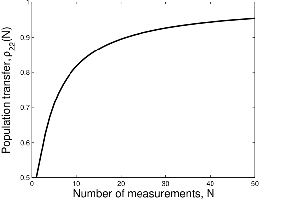
Figure 2: Maximal measurement-induced population transfer from the ground to the excited state of a two-level system as a function of the number of optimal measurements. The maximal population $\rho_{22}(N)$ approaches $1$ as $N\to\infty$.

The function $\rho_{22}(N)$ for $N\leq 50$ is plotted in Fig. 2.

Suppose that the goal is to transfer population $\rho_{22}=1-\varepsilon$ to the excited level, where $\varepsilon\ll 1$. The asymptotic number of optimal measurements necessary to meet this goal may be found as follows:

$$\rho_{22}(N) = 1-\varepsilon\Rightarrow 1+\Bigl{[}\cos\frac{\pi}{N+1}\Bigr{]}^{N+1}=2-2\varepsilon$$

$$\Rightarrow \cos\frac{\pi}{N+1}=(1-2\varepsilon)^{1/(N+1)}\approx 1-\frac{2\varepsilon}{N+1}$$

Notice that a small value of $\varepsilon$ requires $N$ to be large. Therefore the Taylor expansion for $\cos(\pi/(N+1))$ may be used which gives the approximate relation

$$\frac{\pi^{2}}{2(N+1)^{2}}\approx\frac{2\varepsilon}{N+1}$$

It then follows that the number of measurements necessary to transfer population $\rho_{22}=1-\varepsilon$ to the excited level asymptotically behaves as $N\approx\pi^{2}/(4\varepsilon)$, which is consistent with the behavior in Fig. 2 with $N=50$ and $\varepsilon\simeq 0.05$.

Figure 1 illustrates the population transfer by optimal measurements in a two-level system for $N=10$. The left-hand plot corresponds to the case with a non-trivial free dynamics driven by the free Hamiltonian $H_{0}=\frac{1}{2}\sigma_{z}$. The 10 observables $\widetilde{Q}_{1},\dots,\widetilde{Q}_{10}$ are measured at the time moments $t_{k}=Tk/(N+1)$, where the target time is chosen as $T=\pi$, and characterized by the unit norm vectors

$$\widetilde{{\bf a}}^{\rm opt}_{k}=-\cos\Bigl{(}\frac{\pi k}{N+1}\Bigr{)}e_{z}+\sin\Bigl{(}\frac{\pi k}{N+1}\Bigr{)}\Bigl{[}\cos\Bigl{(}\frac{Tk}{N+1}\Bigr{)}e_{x}+\sin\Bigl{(}\frac{Tk}{N+1}\Bigr{)}e_{y}\Bigr{]},\quad k=1,\dots,N$$ (10)

shown on the left-hand plot. The smooth curve passing through the ends of these vectors represents the continuous family of the projectors characterizing the anti-Zeno effect in the limit of infinite number of optimal measurements, as described in the next section.

The right-hand plot in Fig. 1 illustrates the evolution of the system without free dynamics between the measurements. In this case $\varphi_{1}=\dots=\varphi_{11}=\pi/11$ and the optimal observable for the $k$-th measurement is characterized by the vector

$${\bf a}^{\rm opt}_{k}=-\cos\Bigl{(}\frac{\pi k}{N+1}\Bigr{)}e_{z}+\sin\Bigl{(}\frac{\pi k}{N+1}\Bigr{)}e_{x},$$ (11)

which is obtained by rotating the initial vector ${\bf a}_{0}$ by the angle $k\varphi_{1}$. The system density matrix after the $k$-th measurement has the Stokes vector ${\bf b}_{k}\equiv{\bf w}_{10,k}=(\cos\varphi_{1})^{k}{\bf a}^{\rm opt}_{k}$. The plot shows the length of ${\bf b}_{k}$ decreasing after each measurement by the factor $\cos\varphi_{1}$. The relation between the two cases is that each vector $\widetilde{{\bf a}}^{\rm opt}_{k}$ describing optimal $k$-th measurement for the case with free dynamics is obtained by rotating ${\bf a}^{\rm opt}_{k}$ by the angle $\pi k/10$ around $z$-axis. Note that the ten vectors on the left plot of Fig. 1 are the vectors $\widetilde{{\bf a}}^{\rm opt}_{k}$ characterizing the ten optimal measured observables which are measurement-equivalent to the projectors, i.e., pure states, $\widetilde{P}^{\rm opt}_{k}=\frac{1}{2}[\mathbb{I}+\widetilde{{\bf a}}^{\rm opt}_{k}\cdot\sigma]$ and therefore these vectors have unit norm. The ten vectors ${\bf b}_{k}$ on the right plot characterize the system density matrix $\rho=\frac{1}{2}[\mathbb{I}+{\bf b}_{k}\cdot\sigma]$ after each measurement, which is a mixed state due to decoherence induced by the measurements, and therefore these vectors have norm less than one. The shortening of the vectors characterizing the system density matrix after each measurement for the case illustrated on the left plot will be the same, as for the case shown on the right plot, i.e., this shortening is by the factor $\cos\varphi_{1}$ after each measurement.

Numerical simulations for some models in feng also suggest that the expression (9) gives the estimate for the maximal population transfer between any pair of orthogonal levels in any multi-level quantum system. The complete analytical investigation of this problem remains open for a future research.

V Relation with the anti-Zeno effect

The maximal population transfer to the excited level by a finite number of measurements satisfies $\rho_{22}(N)<1$. Since $\lim\limits_{n\to\infty}[\cos(\pi/n)]^{n}=1$, one has $\lim\limits_{N\to\infty}\rho_{22}(N)=1$, i.e., complete population transfer is attained only in the limit of an infinite number of measurements which describes the anti-Zeno effect. To show this behavior consider the projector $E=|1\rangle\langle 1|=\frac{1}{2}[\mathbb{I}+{\bf a}_{0}\cdot\sigma]$. The goal is to steer the system from the initial state $|1\rangle$ at time $t=0$ into the target state $|2\rangle$ at time $t=T$. Define for each $t\in[0,T]$ the unitary operator $U(t)=\exp(i\sigma_{y}\pi t/2T)$. Then $E(t):=U(t)EU^{\dagger}(t)$ is the projector characterized by the Stokes vector ${\bf w}_{t}=-\cos(\pi t/T)e_{z}+\sin(\pi t/T)e_{x}$, i.e., $E(t)=\frac{1}{2}[\mathbb{I}+{\bf w}_{t}\cdot\sigma]$. According to the anti-Zeno effect, continuous measurement of the projector $E(t)$ steers the system at time $t$ into the state characterized by vector ${\bf w}_{t}$. One has ${\bf w}_{\rm T}=e_{z}$, i.e., at the target time the system will be transferred into the state $|2\rangle$.

The anti-Zeno effect is obtained in the limit of an infinite number of measurements when the interval between any two consecutive measurements tends to zero. Consider performing $N$ measurements of the optimal observables $Q^{\rm opt}_{1},\dots,Q^{\rm opt}_{N}$, where $Q^{\rm opt}_{k}=\frac{1}{2}[\mathbb{I}+{\bf a}^{\rm opt}_{k}\cdot\sigma]$ and ${\bf a}^{\rm opt}_{k}$ is defined by Eq. (11). If the dynamics between the measurements is neglected then the state of the system after the $k$-th measurement will be characterized by the vector

$${\bf w}_{N,k}=\Bigl{[}\cos\frac{\pi}{N+1}\Bigr{]}^{k}\Bigl{[}-\cos\Bigl{(}\frac{\pi k}{N+1}\Bigr{)}e_{z}+\sin\Bigl{(}\frac{\pi k}{N+1}\Bigr{)}e_{x}\Bigr{]}$$

Taking the limit as $N,k\to\infty$ such that the ratio $k/(N+1)=t/T$ is kept fixed produces

$$\lim\limits_{N,k\to\infty}{\bf w}_{N,k}=-\cos(\pi t/T)e_{z}+\sin(\pi t/T)e_{x}\equiv{\bf w}_{t}$$

Thus, the anti-Zeno effect is recovered in this limit. The corresponding evolution is characterized by the projector $E(t)$ describing the rotation of the Stokes vector of the system density matrix in the same plane. In general, other evolutions exist which steer the system from the ground to the excited state with projectors $\widetilde{E}(t)$ which induce rotations out of a plane. Such projectors can be limits of optimal control by a finite number of measurements if the free evolution between the measurements is non-trivial. As an example of this situation, the smooth curve on the left plot of Fig. 1 describes the optimal anti-Zeno effect characterized by the projector $\widetilde{E}(t)=\frac{1}{2}[\mathbb{I}+\widetilde{\bf w}_{t}\cdot\sigma]$, where

$$\widetilde{\bf w}_{t}=\lim\limits_{N,k\to\infty}\widetilde{{\bf a}}^{\rm opt}_{k}=-\cos(\pi t/T)e_{z}+\sin(\pi t/T)[\cos(\pi t/T)e_{x}+\sin(\pi t/T)e_{y}]$$

Here the vectors $\widetilde{{\bf a}}^{\rm opt}_{k}$ defined by (10) characterize the optimal measurements for the example with the free evolution considered in Sec. IV, the target time is chosen as $T=\pi$, and the limit is taken with fixed ratio $k/(N+1)=t/T$.

VI Conclusions

In this paper control of quantum systems by non-selective measurements is considered. The capabilities of optimized measurements for control of a two-level system are explicitly investigated. The optimal observables and maximal expectation value of any target observable are analytically found given any initial system density matrix and any fixed number of performed measurements, thus providing a complete analytical solution for control by measurements in a two-level system. For any given number of measurements the degree of control, i.e., the maximum value of the objective, is found. The relation between the optimal measurements and the quantum anti-Zeno effect is established. Looking ahead, the ultimate goal will be specification of laboratory protocols to make the procedure of control by measurement practical for realistic systems.

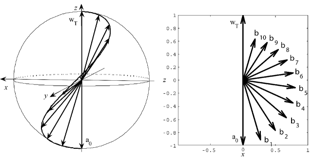
Figure 1: The plots illustrate evolution of a two-level system during the optimal measurement-induced population transfer from the ground to the excited state. The vectors ${\bf a}_{0}=-e_{z}$ and ${\bf w}_{\rm T}=e_{z}$ are the Stokes vectors of the initial and target states. The total number of measurements is $N=10$. The left plot shows the ten unit norm vectors describing the optimal measured observables for a case with non-trivial free system dynamics. The smooth curve passing through the ends of these vectors describes the projectors for the anti-Zeno effect in the limit of an infinite number of optimal measurements. The right plot shows the Stokes vector ${\bf b}_{k}\equiv{\bf w}_{10,k}$, defined by (8), of the system state after $k$ optimal measurements with neglected free dynamics. Each measurement rotates the preceding vector by the angle $\varphi_{1}=\pi/11$ anticlockwise and shortens its length by the factor $\cos\varphi_{1}$.