Separability criteria and bounds for entanglement measures

Abstract

Employing a recently proposed separability criterion we develop analytical lower bounds for the concurrence and for the entanglement of formation of bipartite quantum systems. The separability criterion is based on a nondecomposable positive map which operates on state spaces with even dimension $N\geq 4$, and leads to a class of nondecomposable optimal entanglement witnesses. It is shown that the bounds derived here complement and improve the existing bounds obtained from the criterion of positive partial transposition and from the realignment criterion.

I Introduction

A central problem in quantum information theory ALBER ; ECKERT is the formulation of appropriate measures that quantify the degree of entanglement in composite systems. Particularly important entanglement measures are the concurrence WOOTTERS1 ; WOOTTERS2 ; RUNGTA and the entanglement of formation BENNETT ; VIDAL . These quantities have been widely used in many applications. Examples include studies on the role of entanglement in quantum phase transitions OSTERLOH ; OSBORNE ; LIDAR , on the emergence of long-distance entanglement in spin systems VENUTI , and on additivity properties of the Holevo capacity of quantum channels SHOR .

The explicit determination of most of the proposed entanglement measures for a generic state $\rho$ is an extremely demanding task that requires the solution of a high-dimensional optimization problem. The development of analytical lower bounds for the various entanglement measures is therefore of great interest. Recently, Chen, Albeverio, and Fei ALBEVERIO1 ; ALBEVERIO2 have derived such bounds for the concurrence $C(\rho)$ and for the entanglement of formation $E(\rho)$. They achieved this by relating $C(\rho)$ and $E(\rho)$ to two important and strong separability criteria, namely to the Peres criterion of positive partial transposition (PPT) PERES ; HORODECKI96 and to the realignment criterion CHEN ; RUDOLPH . According to these criteria a given state $\rho$ is entangled (inseparable) if the trace norms $||T_{2}\rho||$ or $||{\mathcal{R}}\rho||$ are strictly larger than 1, where $T_{2}$ denotes the partial transposition and ${\mathcal{R}}$ the realignment transformation. In Refs. ALBEVERIO1 ; ALBEVERIO2 tight lower bounds for $C(\rho)$ and $E(\rho)$ have been formulated in terms of these trace norms.

Here, we extend the connection between separability criteria and entanglement measures to a new criterion which has been developed recently TRC-PAPER . This criterion is based on a universal nondecomposable positive map which leads to a class of optimal entanglement witnesses. Employing these witnesses we derive analytical lower bounds for the concurrence and for the entanglement of formation that can be expressed in terms of a simple linear functional of the given state $\rho$.

The entanglement witnesses constructed here have the special feature of being nondecomposable optimal. This notion has been introduced in Refs. LEWENSTEIN00 ; LEWENSTEIN01 to characterize optimality properties of entanglement witnesses. It means that the witnesses are able to identify entangled PPT states and that no other witnesses exist which can detect more such states. It follows that the bounds developed here can be sharper than those obtained from the PPT criterion and that they are particularly efficient near the border that separates the PPT entangled states from the separable states. In addition, we will demonstrate that they can also be stronger than the bounds given by the realignment criterion. Hence, the new bounds complement and considerably improve the existing bounds.

The paper is organized as follows. In Sec. II we introduce a new separability criterion which is based on a nondecomposable positive map that operates on the states of Hilbert spaces with even dimension $N\geq 4$. We formulate and prove the most important properties of this map, and derive the associated class of optimal entanglement witnesses. Analytical lower bounds for the concurrence are developed in Sec. III. In Sec. IV we discuss an example of a certain family of states in arbitrary dimensions. It will be demonstrated explicitly with the help of this example that the new bounds can be much sharper than the bounds of the PPT and of the realignment criterion. The new class of entanglement witnesses is used in Sec. V to develop corresponding lower bounds for the entanglement of formation. Finally, some conclusions are drawn in Sec. VI.

II Separability criteria

We consider a quantum system with finite-dimensional Hilbert space ${\mathbb{C}}^{N}$. Without loss of generality one can regard ${\mathbb{C}}^{N}$ as the state space of a particle with a certain spin $j$, where $N=2j+1$. As usual, the corresponding basis states are denoted by $|j,m\rangle$, where the quantum number $m$ takes on the values $m=-j,-j+1,\ldots,+j$.

II.1 Time reversal transformation

We will develop a necessary condition for the separability of mixed quantum states which employs the symmetry transformation of the time reversal GALINDO . In quantum mechanics the time reversal is to be described by an antiunitary operator $\theta$. As for any antiunitary operator, we can write $\theta=V\theta_{0}$, where $\theta_{0}$ denotes the complex conjugation in the chosen basis $|j,m\rangle$, and $V$ is a unitary operator. In the spin representation introduced above the matrix elements of $V$ are given by $\langle j,m^{\prime}|V|j,m\rangle=(-1)^{j-m}\delta_{m^{\prime},-m}$. For even $N$, i. e., for half-integer spins $j$, this matrix is not only unitary but also skew-symmetric, which means that $V^{T}=-V$, where $T$ denotes the transposition. It follows that $\theta^{2}=-I$ which leads to

$$\langle\varphi|\theta\varphi\rangle=0.$$ (1)

This relation expresses a well-known property of the time reversal transformation $\theta$ which will play a crucial role in the following: For any state vector $|\varphi\rangle$ the time-reversed state $|\theta\varphi\rangle$ is orthogonal to $|\varphi\rangle$. This is a distinguished feature of even-dimensional state spaces, because unitary and skew-symmetric matrices do not exist in state spaces with odd dimension.

The action of the time reversal transformation on an operator $B$ on ${\mathbb{C}}^{N}$ can be expressed by

$$\vartheta B=\theta B^{\dagger}\theta^{-1}=VB^{T}V^{\dagger}.$$ (2)

This defines a linear map $\vartheta$ which transforms any operator $B$ to its time reversed operator $\vartheta B$. For example, if we take the spin operator $\hat{\bm{j}}$ of the spin-$j$ particle this gives the spin flip transformation $\vartheta\hat{\bm{j}}=-\hat{\bm{j}}$.

II.2 Nondecomposable positive maps and optimal entanglement witnesses

A positive map is a linear transformation $\Lambda$ which takes any positive operator $B$ on some state space ${\mathcal{H}}_{2}$ to a positive operator $\Lambda B$, i. e., $B\geq 0$ implies that $\Lambda B\geq 0$. A positive map $\Lambda$ is said to be completely positive if it has the additional property that the map $I\otimes\Lambda$ operating on any composite system with state space ${\mathcal{H}}_{1}\otimes{\mathcal{H}}_{2}$ is again positive, where $I$ denotes the unit map. The physical significance of positive maps in entanglement theory is provided by a fundamental theorem established in Ref. HORODECKI96 . According to this theorem a necessary and sufficient condition for a state $\rho$ to be separable is that the operator $(I\otimes\Lambda)\rho$ is positive for any positive map $\Lambda$. Hence, maps which are positive but not completely positive can be used as indicators for the entanglement of certain sets of states.

An important example for a positive but not completely positive map is given by the transposition map $T$. The inequality $T_{2}\rho\equiv(I\otimes T)\rho\geq 0$ represents a strong necessary condition for separability known as the Peres criterion of positive partial transposition (PPT criterion). The second relation of Eq. (2) shows that the time reversal transformation $\vartheta$ is unitarily equivalent to the transposition map $T$. Hence, the PPT criterion is equivalent to the condition that the partial time reversal $\vartheta_{2}$ is positive:

$$\vartheta_{2}\rho\equiv(I\otimes\vartheta)\rho\geq 0.$$

We define a linear map $\Phi$ which acts on operators $B$ on ${\mathbb{C}}^{N}$ as follows TRC-PAPER

$$\Phi B=({\mathrm{tr}}B)I-B-\vartheta B,$$ (3)

where ${\mathrm{tr}}B$ denotes the trace of $B$ and $I$ is the unit operator. This map has first been introduced in Ref. NtensorN for the special case $N=4$, in order to study the entanglement structure of SU(2)-invariant spin systems SU2 ; SCHLIEMANN .

For any even $N\geq 4$ the map $\Phi$ defined by Eq. (3) has the following features:

(A)

$\Phi$ is a positive but not completely positive map.

(B)

The map $\Phi$ is nondecomposable.

(C)

The entanglement witnesses corresponding to $\Phi$ are nondecomposable optimal.

In the following we briefly explain and prove these statements.

(A) We first demonstrate that $\Phi$ is a positive map. To this end, we have to show that the operator $\Phi(|\varphi\rangle\langle\varphi|)$ is positive for any normalized state vector $|\varphi\rangle$. Using definition (3) we find:

$$\Phi(|\varphi\rangle\langle\varphi|)=I-|\varphi\rangle\langle\varphi|-|\theta\varphi\rangle\langle\theta\varphi|\equiv I-\Pi.$$

Because of Eq. (1) the operator $\Pi$ introduced here represents an orthogonal projection operator which projects onto the subspace spanned by $|\varphi\rangle$ and $|\theta\varphi\rangle$. It follows that also $\Phi(|\varphi\rangle\langle\varphi|)$ is a projection operator and, hence, that it is positive for any normalized state vector $|\varphi\rangle$. This proves that $\Phi$ is a positive map.

We remark that for $N=2$ the projection $\Pi$ is identical to the unit operator such that $\Phi$ is equal to the zero map in this case. For this reason we restrict ourselves to the cases of even $N\geq 4$. It should be emphasized that $\Phi$ would not be positive if we had used the transposition $T$ instead of the time reversal $\vartheta$ in the definition (3).

The positivity of $\Phi$ implies that the inequality

$$\Phi_{2}\rho\equiv(I\otimes\Phi)\rho\geq 0$$ (4)

provides a necessary condition for separability: any state $\rho$ which violates this condition must be entangled. To show that $\Phi$ is not completely positive, i. e., that the condition (4) is nontrivial, we consider the tensor product space ${\mathcal{H}}_{1}\otimes{\mathcal{H}}_{2}={\mathbb{C}}^{N}\otimes{\mathbb{C}}^{N}$ of two spin-$j$ particles. The total spin of the composite system will be denoted by $J$. According to the triangular inequality $J$ takes on the values $J=0,1,\ldots,2j=N-1$. The projection operator which projects onto the manifold of states corresponding to a definite value of $J$ will be denoted by $P_{J}$. In particular, $P_{0}$ represents the one-dimensional projection onto the maximally entangled singlet state $J=0$.

We define a Hermitian operator $W$ by applying $I\otimes\Phi$ to the singlet state:

$$W\equiv N(I\otimes\Phi)P_{0},$$ (5)

where the factor $N$ is introduced for convenience. More explicit expressions for $W$ can be obtained as follows. First, we observe that ${\mathrm{tr}}_{2}P_{0}=I/N$ since $P_{0}$ is a maximally entangled state (${\mathrm{tr}}_{2}$ denotes the partial trace taken over subsystem 2). Second, we note that the partial time reversal of the singlet state is given by the formula NtensorN

$$\vartheta_{2}P_{0}=\frac{1}{N}F=-\frac{1}{N}\sum_{J=0}^{2j}(-1)^{J}P_{J},$$ (6)

where $F$ denotes the swap operator defined by

$$F|\varphi_{1}\rangle\otimes|\varphi_{2}\rangle=|\varphi_{2}\rangle\otimes|\varphi_{1}\rangle.$$ (7)

Using then definition (3) we get

$$W=I-NP_{0}-F.$$ (8)

Another useful representation is obtained by use of the fact that the sum of the $P_{J}$ is equal to the unit operator. Expressing $F$ as shown in Eq. (6) we then find:

$$W=-(N-2)P_{0}+2P_{2}+2P_{4}+\ldots+2P_{2j-1}.$$ (9)

We infer from Eq. (9) that $W$ has the negative eigenvalue $-(N-2)$ corresponding to the singlet state $J=0$. Therefore, the operator $W$ is not positive and, hence, the map $\Phi$ is not completely positive.

(B) Since $\Phi$ is positive but not completely positive the operator $W$ defined in Eq. (5) is an entanglement witness HORODECKI96 ; TERHAL . We recall that an entanglement witness is an observable which satisfies ${\mathrm{tr}}\{W\sigma\}\geq 0$ for all separable states $\sigma$, and ${\mathrm{tr}}\{W\rho\}<0$ for at least one inseparable state $\rho$, in which case we say that $W$ detects $\rho$.

An entanglement witness $W$ is called nondecomposable if it can detect entangled PPT states LEWENSTEIN00 , i. e., if there exist PPT states $\rho$ that satisfy ${\mathrm{tr}}\{W\rho\}<0$. We will demonstrate in Sec. IV by means of an explicit example that there are always such states for the witness defined by Eq. (5). It follows that our witness $W$ is nondecomposable. This implies that also the map $\Phi$ is nondecomposable WORONOWICZ , and that the criterion (4) is able to detect entangled PPT states.

(C) The observable $W$ introduced above has a further remarkable optimality property. To explain this property we introduce the following notation LEWENSTEIN00 . We denote by $D_{W}$ the set of all entangled PPT states of the total state space which are detected by some given nondecomposable witness $W$. A witness $W_{2}$ is said to be finer than a witness $W_{1}$ if $D_{W_{1}}$ is a subset of $D_{W_{2}}$, i. e., if all entangled PPT states which are detected by $W_{1}$ are also detected by $W_{2}$. A given witness is said to be nondecomposable optimal if there is no other witness which is finer, i. e., if there is no other witness which is able to detect more entangled PPT states.

It can be shown that the witness $W$ defined by (5) is always optimal in this sense. The proof can be carried out by showing that the set of product vectors $|\varphi_{1},\varphi_{2}\rangle$ satisfying $\langle\varphi_{1},\varphi_{2}|W|\varphi_{1},\varphi_{2}\rangle=0$ spans the total Hilbert space. The details of the proof are given in Ref. TRC-PAPER .

III Bounds for the concurrence

The generalized concurrence of a pure state $\rho=|\psi\rangle\langle\psi|$ is defined by RUNGTA

$$C(|\psi\rangle)=\sqrt{2(1-{\mathrm{tr}}_{1}\rho_{1}^{2})},$$

where $\rho_{1}={\mathrm{tr}}_{2}\rho$ represents the reduced density matrix of subsystem 1, given by the partial trace taken over subsystem 2. We consider the Schmidt decomposition

$$|\psi\rangle=\sum_{i}\alpha_{i}|\varphi_{i}\rangle\otimes|\chi_{i}\rangle,$$ (10)

where $\{|\varphi_{i}\rangle\}$ and $\{|\chi_{i}\rangle\}$ are orthonormal bases in ${\mathcal{H}}_{1}$ and ${\mathcal{H}}_{2}$, respectively, and the $\alpha_{i}$ are the Schmidt coefficients satisfying $\alpha_{i}\geq 0$ and the normalization condition

$$\sum_{i}\alpha_{i}^{2}=1.$$ (11)

The concurrence can then be expressed in terms of the Schmidt coefficients:

$$C(|\psi\rangle)=\sqrt{2\sum_{i\neq j}\alpha_{i}^{2}\alpha_{j}^{2}}.$$ (12)

For a mixed state $\rho$ the concurrence is defined to be

$$C(\rho)={\mathrm{min}}\left\{\sum_{r}p_{r}C(|\psi_{r}\rangle)\;\Big{|}\;\rho=\sum_{r}p_{r}|\psi_{r}\rangle\langle\psi_{r}|\right\},$$ (13)

where the minimum is taken over all possible convex decompositions of $\rho$ into an ensemble $\{|\psi_{r}\rangle\}$ of pure states with probability distribution $\{p_{r}\}$.

Let $\rho=\sum_{r}p_{r}|\psi_{r}\rangle\langle\psi_{r}|$ be an optimal decomposition of $\rho$ for which the minimum of Eq. (13) is attained. Denoting the Schmidt coefficients of $|\psi_{r}\rangle$ by $\alpha_{i}^{r}$ we then have:

$$C(\rho) = \sum_{r}p_{r}C(|\psi_{r}\rangle)$$ (14)

$$= \sum_{r}p_{r}\sqrt{2\sum_{i\neq j}(\alpha_{i}^{r})^{2}(\alpha_{j}^{r})^{2}}$$

$$\geq \sum_{r}p_{r}\sqrt{\frac{2}{N(N-1)}}\sum_{i\neq j}\alpha_{i}^{r}\alpha_{j}^{r}.$$

In the second line we have used Eq. (12), and the third line is obtained with the help of the inequality

$$\sum_{i\neq j}\alpha_{i}^{2}\alpha_{j}^{2}\geq\frac{1}{N(N-1)}\left(\sum_{i\neq j}\alpha_{i}\alpha_{j}\right)^{2},$$

which holds for any set of $N$ numbers $\alpha_{i}$ ALBEVERIO1 .

Consider now any real-valued and convex functional $f(\rho)$ on the total state space with the following property. For all state vectors $|\psi\rangle$ with Schmidt decomposition (10) we have:

$$f(|\psi\rangle\langle\psi|)\leq\sum_{i\neq j}\alpha_{i}\alpha_{j}.$$ (15)

Given such a functional we can continue inequality (14) as follows:

$$C(\rho) \geq \sqrt{2/N(N-1)}\sum_{r}p_{r}\sum_{i\neq j}\alpha_{i}^{r}\alpha_{j}^{r}$$

$$\geq \sqrt{2/N(N-1)}\sum_{r}p_{r}f(|\psi_{r}\rangle\langle\psi_{r}|)$$

$$\geq \sqrt{2/N(N-1)}f\left(\sum_{r}p_{r}|\psi_{r}\rangle\langle\psi_{r}|\right)$$

$$= \sqrt{2/N(N-1)}f(\rho).$$

In the second line we have used inequality (15), and in the third line the convexity of $f(\rho)$.

We conclude that any convex functional $f(\rho)$ with the property (15) leads to a lower bound for the concurrence:

$$C(\rho)\geq\sqrt{\frac{2}{N(N-1)}}f(\rho).$$

In Ref. ALBEVERIO1 two example for such a functional $f(\rho)$ have been constructed which are based on the PPT criterion and on the realignment criterion:

$$f_{\mathrm{ppt}}(\rho) = ||T_{2}\rho||-1,$$

$$f_{\mathrm{realign}}(\rho) = ||{\mathcal{R}}\rho||-1,$$

where $T_{2}$ denotes the partial transposition and ${\mathcal{R}}$ the realignment transformation. These functionals are convex because of the convexity of the trace norm which is defined by $||A||={\mathrm{tr}}\sqrt{A^{\dagger}A}$. Moreover, for both functionals the equality sign of Eq. (15) holds:

$$f_{\mathrm{ppt}}(|\psi\rangle\langle\psi|)=f_{\mathrm{realign}}(|\psi\rangle\langle\psi|)=\sum_{i\neq j}\alpha_{i}\alpha_{j}.$$ (16)

Consider the functional

$$f_{W}(\rho)=-{\mathrm{tr}}(W\rho),$$

where $W$ is the entanglement witness introduced in Eq. (5). This functional is linear and of course convex. We claim that $f_{W}(\rho)$ also satisfies the bound (15), i. e., for any state vector $|\psi\rangle$ with Schmidt decomposition (10) we have

$$f_{W}(|\psi\rangle\langle\psi|)\equiv-\langle\psi|W|\psi\rangle\leq\sum_{i\neq j}\alpha_{i}\alpha_{j}.$$ (17)

To show this we first determine the expectation value of $W$. From Eq. (6) we have $NP_{0}=\vartheta_{2}F$ and, hence, the expression (8) can be written as $W=I-F-\vartheta_{2}F$. This gives

$$\langle\psi|W|\psi\rangle=1-\langle\psi|F|\psi\rangle-\langle\psi|\vartheta_{2}F|\psi\rangle.$$

With the help of the definitions of the swap operator $F$ [Eq. (7)] and of the time reversal transformation [Eq. (2)] it is easy to verify the formulae

$$\langle\psi|F|\psi\rangle = \sum_{ij}\alpha_{i}\alpha_{j}\langle\varphi_{i}|\chi_{j}\rangle\langle\chi_{i}|\varphi_{j}\rangle,$$

$$\langle\psi|\vartheta_{2}F|\psi\rangle = \sum_{ij}\alpha_{i}\alpha_{j}\langle\varphi_{i}|\theta\chi_{i}\rangle\langle\theta\chi_{j}|\varphi_{j}\rangle.$$

This leads to

$$\langle\psi|W|\psi\rangle=1-\sum_{ij}\alpha_{i}\alpha_{j}A_{ij},$$

where

$$A_{ij}\equiv\langle\varphi_{i}|\chi_{j}\rangle\langle\chi_{i}|\varphi_{j}\rangle+\langle\varphi_{i}|\theta\chi_{i}\rangle\langle\theta\chi_{j}|\varphi_{j}\rangle.$$ (18)

Hence, we have

$$f_{W}(|\psi\rangle\langle\psi|)=\sum_{ij}\alpha_{i}\alpha_{j}A_{ij}-1\leq\sum_{ij}\alpha_{i}\alpha_{j}|A_{ij}|-1.$$

It is shown in Appendix A that

$$|A_{ij}|\leq 1.$$ (19)

This leads immediately to the desired inequality:

$$f_{W}(|\psi\rangle\langle\psi|)\leq\sum_{ij}\alpha_{i}\alpha_{j}-1=\sum_{i\neq j}\alpha_{i}\alpha_{j},$$

where we have used the normalization condition (11).

Summarizing we have obtained the following lower bound for the concurrence:

$$C(\rho)\geq-\sqrt{\frac{2}{N(N-1)}}{\mathrm{tr}}(W\rho).$$ (20)

Of course, this bound is only nontrivial if $\rho$ is detected by the entanglement witness $W$, i. e., if ${\mathrm{tr}}(W\rho)<0$. It will be demonstrated in Sec. IV that this bound can be much stronger than the bounds given by $f_{\mathrm{ppt}}$ and $f_{\mathrm{realign}}$, which is due to the fact $W$ identifies many entangled states that are neither detected by the PPT criterion nor by the realignment criterion.

IV Example

We illustrate the application of the inequality (20) with the help of a certain family of states. This family contains a separable state, entangled PPT states, as well as entangled states whose partial transposition is not positive. The example will also lead to a proof of the claim that the map $\Phi$ and the witness $W$ are nondecomposable.

Consider the following one-parameter family of states:

$$\rho(\lambda)=\lambda P_{0}+(1-\lambda)\rho_{0},\qquad 0\leq\lambda\leq 1.$$ (21)

These normalized states are mixtures of the singlet state $P_{0}$ and of the state

$$\rho_{0}=\frac{2}{N(N+1)}P_{S}=\frac{2}{N(N+1)}\sum_{J\;\mathrm{odd}}P_{J},$$

where $P_{S}$ denotes the projection onto the symmetric subspace under the swap operation $F$. We note that $\rho_{0}$ is a separable state which belongs to the class of the Werner states WERNER . Since $P_{S}$ can be written as a sum over the projections $P_{J}$ with odd $J$, we immediately get with the help of Eq. (5):

$${\mathrm{tr}}(W\rho(\lambda))=-\lambda(N-2).$$ (22)

Hence, we find that ${\mathrm{tr}}(W\rho(\lambda))<0$ for $\lambda>0$. It follows that all states of the family (21) corresponding to $\lambda>0$ are entangled, and that $\rho_{0}$ is the only separable state of this family.

Employing Eqs. (22) and (20) we get the following lower bound for the concurrence:

$$C(\rho(\lambda))\geq\sqrt{\frac{2(N-1)}{N}}\frac{N-2}{N-1}\lambda.$$ (23)

To compare this bound with those obtained from the PPT and the realignment criterion we have to determine the trace norms $||T_{2}\rho(\lambda)||$ and $||{\mathcal{R}}\rho(\lambda)||$. The details of the calculation are presented in Appendix B. One finds that the PPT criterion gives the bounds:

$$C(\rho(\lambda))\geq$$ (28)

$$\left\{\begin{array}[]{ll}0,&\lambda\leq\frac{1}{N+2}\\ \sqrt{\frac{2(N-1)}{N}}\frac{N-2}{N(N-1)}\left[(N+2)\lambda-1\right],&\frac{1}{N+2}\leq\lambda\leq\frac{1}{2}\\ \sqrt{\frac{2(N-1)}{N}}\frac{N\lambda-1}{N-1},&\frac{1}{2}\leq\lambda\end{array}\right.$$

while the realignment criterion yields:

$$C(\rho(\lambda))\geq\left\{\begin{array}[]{ll}\sqrt{\frac{2(N-1)}{N}}\frac{-2\lambda}{N-1},&\lambda\leq\frac{1}{N+2}\\ \sqrt{\frac{2(N-1)}{N}}\frac{N\lambda-1}{N-1},&\frac{1}{N+2}\leq\lambda\end{array}\right.$$ (29)

The relations (23)-(29) lead to a number of important conclusions. First of all, we observe from Eq. (28) that the states within the range $\lambda\leq 1/(N+2)$ have positive partial transposition (in this range $||T_{2}\rho(\lambda)||$ is equal to $1$, see Appendix B). But from Eq. (22) we know that all states with $\lambda>0$ must be entangled. It follows that all states in the range $0<\lambda\leq 1/(N+2)$ are entangled PPT states which are detected by the witness $W$. This proves, as claimed in Sec. II, that the witness $W$ and, hence, also the map $\Phi$ are nondecomposable.

According to Eq. (28) the PPT criterion only detects the entanglement of the states with $\lambda>1/(N+2)$. It is thus weaker than the criterion based on the witness $W$. As can be seen from Eq. (29) the realignment criterion is even weaker because it only recognizes the entanglement of the states with $\lambda>1/N$ (the trace norm of ${\mathcal{R}}\rho(\lambda)$ is larger than $1$ if and only if $\lambda>1/N$, see Appendix B).

A plot of the various lower bounds for the example $N=4$ is shown in Fig. 1. We see that the new bound (23) is the best one within the range $\lambda<1/2$. The bounds given by the PPT and the realignment criterion coincide in the range $\lambda>1/2$. In this range they are better than the new bound. Note that these features hold true for all $N$. We remark that for large $N$ the concurrence approaches the limit $C(\rho(\lambda))=\sqrt{2}\lambda$.

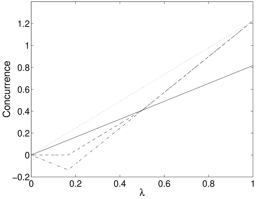
Figure 1: Concurrence of the states (21) for $N=4$. Solid line: The new lower bound given by Eq. (23). Dashed line: Lower bound given by the PPT criterion [Eq. (28)]. Dashed-dotted line: Lower bound given by the realignment criterion [Eq. (29)]. Dotted line: Upper bound given by $C(\rho(\lambda))\leq\sqrt{2(N-1)/N}\lambda$.

V Entanglement of formation

For a pure state $|\psi\rangle$ with Schmidt decomposition (10) one defines the entanglement of formation by

$$E(|\psi\rangle)=H(\bm{\alpha})\equiv-\sum_{i}\alpha_{i}^{2}\log\alpha_{i}^{2},$$

where $\bm{\alpha}$ denotes the vector of the Schmidt coefficients, and $\log$ is the base $2$ logarithm. The quantity $H(\bm{\alpha})$ is the Shannon entropy of the distribution $\alpha_{i}^{2}$, which is equal to the von Neumann entropy of the reduced density matrices. This definition is extended to mixed states through the convex hull construction:

$$E(\rho)={\mathrm{min}}\left\{\sum_{r}p_{r}E(|\psi_{r}\rangle)\;\Big{|}\;\rho=\sum_{r}p_{r}|\psi_{r}\rangle\langle\psi_{r}|\right\},$$

where the minimum is again taken over all possible convex decompositions of $\rho$.

An analytical lower bound for the entanglement of formation has been constructed in Ref. ALBEVERIO2 , which may be described as follows. First, for $1\leq\Lambda\leq N$ one defines the function

$$R(\Lambda)=\min_{\bm{\alpha}}\left\{H(\bm{\alpha})\;\Big{|}\;\sum_{ij}\alpha_{i}\alpha_{j}=\Lambda\right\}.$$

The minimum is taken over all Schmidt vectors $\bm{\alpha}$, i. e., $R(\Lambda)$ is the minimal value of the entropy $H(\bm{\alpha})$ under the constraint $\sum_{ij}\alpha_{i}\alpha_{j}=\Lambda$. The solution of this minimization problem has been derived by Terhal and Vollbrecht TERHAL-VOLLBRECHT :

$$R(\Lambda)=H_{2}(\gamma(\Lambda))+[1-\gamma(\Lambda)]\log(N-1),$$

where

$$\gamma(\Lambda)=\frac{1}{N^{2}}\left[\sqrt{\Lambda}+\sqrt{(N-1)(N-\Lambda)}\right]^{2},$$

and

$$H_{2}(x)=-x\log x-(1-x)\log(1-x)$$

is the binary entropy. Second, one introduces the convex hull ${\mathrm{co}}[R(\Lambda)]$ of $R(\Lambda)$. This is the largest convex function which is bounded from above by $R(\Lambda)$. One then gets the following lower bound for the entanglement of formation:

$$E(\rho) \geq {\mathrm{co}}[R(\Lambda_{0})],$$

$$\Lambda_{0} \equiv {\mathrm{max}}\left\{||T_{2}\rho||,||{\mathcal{R}}\rho||\right\}.$$ (30)

The decisive point of the construction given in Ref. ALBEVERIO2 is the fact that [see Eq. (16)]

$$||T_{2}(|\psi\rangle\langle\psi|)||=||{\mathcal{R}}(|\psi\rangle\langle\psi|)||=\sum_{ij}\alpha_{i}\alpha_{j}=\Lambda.$$

This means that the function $R(\Lambda)$ yields the minimal entropy $H(\bm{\alpha})$ under the constraint of a fixed value $\Lambda$ for the trace norm $||T_{2}(|\psi\rangle\langle\psi|)||$ or $||{\mathcal{R}}(|\psi\rangle\langle\psi|)||$. But from Eq. (17) we also have

$$1-\langle\psi|W|\psi\rangle\leq\sum_{ij}\alpha_{i}\alpha_{j}=\Lambda.$$

By use of this inequality one can immediately repeat the proof of Ref. ALBEVERIO2 , replacing the trace norm $||T_{2}\rho||$ or $||{\mathcal{R}}\rho||$ by the quantity $1-{\mathrm{tr}}(W\rho)$. Hence, we are led to a sharper bound for the entanglement of formation:

$$E(\rho) \geq {\mathrm{co}}[R(\Lambda_{0})],$$

$$\Lambda_{0} \equiv {\mathrm{max}}\left\{||T_{2}\rho||,||{\mathcal{R}}\rho||,1-{\mathrm{tr}}(W\rho)\right\}.$$ (31)

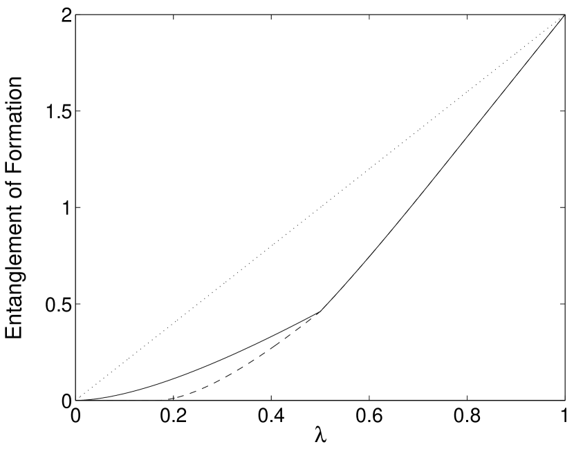
Figure 2: Entanglement of formation of the states (21) for $N=4$. Solid line: The new lower bound given by Eqs. (V)-(33). Dashed line: Lower bound given by Eq. (V). Dotted line: Upper bound given by $E(\rho(\lambda))\leq\lambda\log N$.

Let us apply this result to the family of states given in Eq. (21). In this case we have:

$$\Lambda_{0}=\max\left\{N\lambda,(N-2)\lambda+1\right\}.$$

By use of the Terhal-Vollbrecht conjecture TERHAL-VOLLBRECHT on the form of the function ${\mathrm{co}}[R(\Lambda)]$ (see also Ref. FEI ) we get:

$$E(\rho(\lambda))\geq H_{2}(\gamma(\Lambda_{0}))+[1-\gamma(\Lambda_{0})]\log(N-1)$$ (32)

for $1\leq\Lambda_{0}\leq 4(N-1)/N$, and

$$E(\rho(\lambda))\geq\frac{\log(N-1)}{N-2}(\Lambda_{0}-N)+\log N$$ (33)

for $4(N-1)/N\leq\Lambda_{0}\leq N$. The general features of this result are similar to those discussed within the context of the concurrence. The special case $N=4$ is plotted in Fig. 2. We finally note that

$$E(\rho(\lambda))\sim\lambda\log N$$

represents the asymptotic limit of the entanglement of formation for large $N$.

VI Conclusions

By use of a universal positive map $\Phi$ we have obtained a class of nondecomposable optimal entanglement witnesses $W$. Employing these witnesses analytical bounds for the concurrence and for the entanglement of formation have been developed. Similar bounds can be derived for other measures, e. g., for the entanglement measure which is known as tangle CAVES . Due to the fact that $W$ is a nondecomposable optimal entanglement witness, the bounds obtained here are particularly good near the boundary which separates the region of classically correlated states from the region of entangled states with positive partial transposition.

It should be clear from the general considerations in Secs. III and V and from the example of Sec. IV that the bounds derived here are not intended to replace other known bounds, but rather to complement these. In fact, the bounds based on the witness $W$ can be weaker than those given by PPT or the realignment criterion, in particular in those cases in which the optimal decomposition of $\rho$ consists entirely of maximally entangled states. To give an example, we consider the family of states which are invariant under all unitary product transformations of the form $U\otimes U^{*}$, were $U^{*}$ denotes the complex conjugation of $U$. These states, known as isotropic states HORODECKI99 , can be parameterized by a single parameter, namely by their fidelity $f\in[0,1]$. The isotropic states for $f\leq 1/N$ are separable and for $f>1/N$ their concurrence is given by CAVES

$$C(f)=\sqrt{\frac{2N}{N-1}}\left(f-\frac{1}{N}\right).$$ (34)

The right-hand side of this equation coincides with the bound given by the PPT criterion, i. e., the application of the latter already yields the exact expression for the concurrence ALBEVERIO1 . On the other hand, the bound given by Eq. (20) yields

$$C(f)\geq\sqrt{\frac{2N}{N-1}}\frac{N-2}{N-1}\left(f-\frac{1}{N}\right).$$ (35)

Since the right-hand side is strictly larger than zero for $f>1/N$ we can conclude that, like the PPT criterion, also the new criterion (4) provides a necessary and sufficient condition for the separability of the isotropic states. But if we compare Eqs. (34) and (35) we see that the bound obtained by the witness $W$ is always weaker than the bound of the PPT criterion. Note however that for large $N$ the difference between these bounds is only of order $1/N$.

We finally indicate some generalizations of the present approach. An obvious extension concerns the definition of the entanglement witness $W$ given by Eq. (5). According to this definition the witness $W$ depends of course on the chosen basis and is not invariant under local unitary transformations. However, for any product transformation $U=U_{1}\otimes U_{2}$ with unitary operators $U_{1}$ and $U_{2}$ the observable $W_{U}=UWU^{\dagger}$ is again an entanglement witness. It is clear from the proof given in Appendix A that for arbitrary $U_{1}$ and $U_{2}$ the witness $W_{U}$ also satisfies the inequality (17). It follows that we may perform the replacement

$${\mathrm{tr}}(W\rho)\longrightarrow\min_{U}\{{\mathrm{tr}}(W_{U}\rho)\}$$

in the bounds for the concurrence [Eq. (20)] and for the entanglement of formation [Eq. (V)], where the minimum is taken over all product unitaries $U=U_{1}\otimes U_{2}$. This replacement sharpens the lower bounds and ensures that they are invariant under local unitary operations.

For simplicity we have restricted ourselves to the case of bipartite systems with state space ${\mathbb{C}}^{N}\otimes{\mathbb{C}}^{N}$. The definition $W=N(I\otimes\Phi)P_{0}$ for the witness $W$ can be extended to state spaces ${\mathbb{C}}^{M}\otimes{\mathbb{C}}^{N}$ with arbitrary $M>N$ in an obvious way, replacing the singlet state $P_{0}$ by any maximally entangled pure state in ${\mathbb{C}}^{M}\otimes{\mathbb{C}}^{N}$. Moreover, an extension of the present approach to state spaces with odd dimension $N$ seems to be possible. To this end one has to drop the condition that the operator $V$ introduced in Sec. II.1 is unitary, i. e., one only requires that $V$ is skew-symmetric and that $V^{\dagger}V\leq I$. It is worth investigating applications of these constructions to bipartite and multipartite quantum systems.

Appendix A Proof of inequality (19)

To prove inequality (19) we consider a fixed pair $(i,j)$ of indices and decompose $|\theta\chi_{i}\rangle$ into a component which is parallel to $|\chi_{j}\rangle$ and a component which is perpendicular to $|\chi_{j}\rangle$:

$$|\theta\chi_{i}\rangle=\lambda|\chi_{j}\rangle+\mu|\chi_{j}^{\perp}\rangle,$$ (36)

where $\langle\chi_{j}|\chi_{j}^{\perp}\rangle=0$ and $|\lambda|^{2}+|\mu|^{2}=1$. Applying the time reversal transformation to this equation we get:

$$|\chi_{i}\rangle=-\lambda^{*}|\theta\chi_{j}\rangle-\mu^{*}|\theta\chi_{j}^{\perp}\rangle.$$ (37)

Inserting (36) and (37) into the expression (18) one obtains:

$$A_{ij}=\mu\left[\langle\varphi_{i}|\chi_{j}\rangle\langle\theta\varphi_{j}|\chi_{j}^{\perp}\rangle-\langle\varphi_{i}|\chi_{j}^{\perp}\rangle\langle\theta\varphi_{j}|\chi_{j}\rangle\right].$$

Since $|\mu|\leq 1$ this leads to

$$|A_{ij}|\leq ab+cd,$$

where we have introduced the quantities:

$$a=|\langle\varphi_{i}|\chi_{j}\rangle|, \qquad b=|\langle\theta\varphi_{j}|\chi_{j}^{\perp}\rangle|,$$

$$c=|\langle\varphi_{i}|\chi_{j}^{\perp}\rangle|, \qquad d=|\langle\theta\varphi_{j}|\chi_{j}\rangle|.$$

Since $|\chi_{j}\rangle$ is perpendicular to $|\chi_{j}^{\perp}\rangle$ by construction, we have

$$a^{2}+c^{2}=|\langle\varphi_{i}|\chi_{j}\rangle|^{2}+|\langle\varphi_{i}|\chi_{j}^{\perp}\rangle|^{2}\leq 1,$$

and, therefore, $c\leq\sqrt{1-a^{2}}$. In a similar manner we get $d\leq\sqrt{1-b^{2}}$. Hence, we obtain:

$$|A_{ij}|\leq ab+\sqrt{1-a^{2}}\sqrt{1-b^{2}}.$$

It is easy to see that the right-hand side of this inequality is smaller than or equal to 1 for all $a,b\in[0,1]$, which yields the desired inequality (19).

Appendix B Determination of the trace norms $||T_{2}\rho(\lambda)||$ and $||{\mathcal{R}}\rho(\lambda)||$

Since $T_{2}\rho$ and $\vartheta_{2}\rho$ are unitarily equivalent we have $||T_{2}\rho(\lambda)||=||\vartheta_{2}\rho(\lambda)||$. Using Eqs. (21) and (6), and the representation $P_{S}=(I+F)/2$ we get

$$\vartheta_{2}\rho(\lambda)=\frac{1-2\lambda}{N}P_{0}+\frac{1}{N}\sum_{J=1}^{2j}\left[(-1)^{J+1}\lambda+\frac{1-\lambda}{N+1}\right]P_{J}.$$

Hence, the trace norm of $T_{2}\rho(\lambda)$ is found to be:

$$||T_{2}\rho(\lambda)||=\frac{|1-2\lambda|}{N}+\sum_{J=1}^{2j}\frac{2J+1}{N}\left|(-1)^{J+1}\lambda+\frac{1-\lambda}{N+1}\right|.$$

Carrying out this sum one gets:

$$||T_{2}\rho(\lambda)||-1=\left\{\begin{array}[]{ll}0,&\lambda\leq\frac{1}{N+2}\\ \frac{N-2}{N}\left[(N+2)\lambda-1\right],&\frac{1}{N+2}\leq\lambda\leq\frac{1}{2}\\ N\lambda-1,&\frac{1}{2}\leq\lambda\end{array}\right.$$

which yields the lower bounds of Eq. (28).

To determine $||{\mathcal{R}}\rho(\lambda)||$ we note that the realignment transformation may be written as ${\mathcal{R}}\rho=\vartheta_{2}(F\rho)$. Using $FP_{0}=-P_{0}$ and $FP_{S}=P_{S}$ one easily deduces that

$${\mathcal{R}}\rho(\lambda)=\frac{1}{N}P_{0}+\frac{1}{N}\sum_{J=1}^{2j}\left[(-1)^{J}\lambda+\frac{1-\lambda}{N+1}\right]P_{J},$$

which yields:

$$||{\mathcal{R}}\rho(\lambda)||=\frac{1}{N}+\sum_{J=1}^{2j}\frac{2J+1}{N}\left|(-1)^{J}\lambda+\frac{1-\lambda}{N+1}\right|.$$

The evaluation of this sum leads to:

$$||{\mathcal{R}}\rho(\lambda)||-1=\left\{\begin{array}[]{ll}-2\lambda,&\lambda\leq\frac{1}{N+2}\\ N\lambda-1,&\frac{1}{N+2}\leq\lambda\end{array}\right.$$

which gives the lower bounds of Eq. (29).

References

- (1) G. Alber, T. Beth, M. Horodecki, P. Horodecki, R. Horodecki, M. Rötteler, H. Weinfurter, R. Werner, and A. Zeilinger, Quantum Information (Springer-Verlag, Berlin, 2001).
- (2) K. Eckert, O. Gühne, F. Hulpke, P. Hyllus, J. Korbicz, J. Mompart, D. Bruß, M. Lewenstein, and A. Sanpera, in Quantum Information Processing, edited by G. Leuchs and T. Beth (Wiley-VCH, Berlin, 2005).
- (3) W. K. Wootters, Phys. Rev. Lett. 80, 2245 (1998).
- (4) W. K. Wootters, Quant. Inf. Comp. 1, 27 (2001).
- (5) P. Rungta, V. Bužek, C. M. Caves, M. Hillery, and G. J. Milburn, Phys. Rev. A 64, 042315 (2001).
- (6) C. H. Bennett, D. P. DiVincenzo, J. A. Smolin, and W. K. Wootters, Phys. Rev. A 54, 3824 (1996).
- (7) G. Vidal, J. Mod. Opt. 47, 355 (2000).
- (8) A. Osterloh, L. Amico, G. Falci, and R. Fazio, Nature 416, 608 (2002).
- (9) T. J. Osborne and M. A. Nielsen, Phys. Rev. A 66, 032110 (2002).
- (10) L.-A. Wu, M. S. Sarandy, and D. A. Lidar, Phys. Rev. Lett. 93, 250404 (2004).
- (11) L. Campos Venuti, C. Degli Esposti Boschi, and M. Roncaglia, eprint quant-ph/0604215.
- (12) P. W. Shor, Commun. Math. Phys. 246, 453 (2004).
- (13) K. Chen, S. Albeverio, and S.-M. Fei, Phys. Rev. Lett. 95, 040504 (2005).
- (14) K. Chen, S. Albeverio, and S.-M. Fei, Phys. Rev. Lett. 95, 210501 (2005).
- (15) A. Peres, Phys. Rev. Lett. 77, 1413 (1996).
- (16) M. Horodecki, P. Horodecki, and R. Horodecki, Phys. Lett. A 223, 1 (1996).
- (17) K. Chen and L.-A. Wu, Quant. Inf. Comp. 3, 193 (2003).
- (18) O. Rudolph, Phys. Rev. A 67, 032312 (2003).
- (19) H. P. Breuer, eprint quant-ph/0605036.
- (20) M. Lewenstein, B. Kraus, J. I. Cirac, and P. Horodecki, Phys. Rev. A 62, 052310 (2000).
- (21) M. Lewenstein, B. Kraus, P. Horodecki, and J. I. Cirac, Phys. Rev. A 63, 044304 (2001).
- (22) A. Galindo and P. Pascual, Quantum Mechanics I (Springer-Verlag, Berlin, 1990).
- (23) H. P. Breuer, Phys. Rev. A 71, 062330 (2005).
- (24) H. P. Breuer, J. Phys. A 38, 9019 (2005).
- (25) J. Schliemann, Phys. Rev. A 72, 012307 (2005).
- (26) B. M. Terhal, Phys. Lett. A 271, 319 (2000).
- (27) S. L. Woronowicz, Rep. Math. Phys. 10, 165 (1976).
- (28) R. F. Werner, Phys. Rev. A 40, 4277 (1989).
- (29) B. M. Terhal and K. G. H. Vollbrecht, Phys. Rev. Lett. 85, 2625 (2000).
- (30) S.-M. Fei and X. Li-Jost, Phys. Rev. A 73, 024302 (2006).
- (31) P. Rungta and C. M. Caves, Phys. Rev. A 67, 012307 (2003).
- (32) M. Horodecki and P. Horodecki, Phys. Rev. A 59, 4206 (1999).