Quantum interference and evolution of entanglement in a system of three-level atoms

Abstract

We consider a pair of three-level atoms interacting with the vacuum. The process of disentanglement due to spontaneous emission and the role of quantum interference between principal transitions in this process, are analysed. We show that the presence of interference can slow down disentanglement. In the limit of maximal interference, some part of initial entanglement can survive.

I Introduction

The process of decoherence and degradation of entanglement in open quantum systems was studied mainly in the case of pair of two-level atoms interacting with vacuum or thermal noises. This system is simple to study, since the amount of its entanglement can be quantified by concurrence wootters . This quantity discriminates between separable and entangled states and is analytically computable. The dynamics of the system given in the Markovian regime by the master equation, can be used to obtain time evolution of concurrence and to analyse the influence of the process of decoherence on entanglement. Let us mention two particular results of such studies. The process of disentanglement was considered in the case of a pair of atoms, each interacting with its own reservoir at zero temperature. It turns out that concurrence of initially entangled state can vanish asymptotically or in finite time, depending on initial state eberly ; dodd ; jam . This behaviour should be compared with asymptotic decoherence of any initial state. On the other hand, individual atoms located inside two independent environments at infinite temperatures, always disentangle at finite times jajam .

In the present paper, we extend this kind of studies to the case of pair of three-level atoms. The analysis is much more involved since there is no simple necessary and sufficient criterion of entanglement for a pair of $d$-level systems with $d\geq 3$. Peres’ separability criterion peres only shows that states which are not positive after partial transposition (NPPT states) are entangled. But there can exist entangled states which are positive after this operation horodecki (PPT states). Using this criterion we at most can study the evolution of NPPT states and ask when they become PPT states, but in the models considered in the present paper we can directly observe when stationary asymptotic states are separable.

Interesting example of dissipative dynamics comes from the analysis of three-level V-type atomic system where spontaneous emission may take place from two excited levels to the ground state and direct transition between excited levels is not allowed. However the indirect coupling between excited states can appear due to interaction with the vacuum (quantum interference) agarwal . This interference results from the following mechanism: spontaneous emission from one transition modifies spontaneous emission from the other transition ficek . There were many studies on the effect of quantum interference on various processes including: resonance fluorescence heg , quantum jumps zoller , the presence of ultranarrow spectral lines swain or amplification without population inversion harris .

In our research we consider a pair of such three-level systems and study another aspect of quantum interference, namely its influence on the evolution of entangled states. In the case of distant atoms we expect that dissipation causes disentanglement, but the rate of this process may depend on interference. It is indeed true, as shows analysis of the models considered in the paper. We demonstrate it for some classes of pure and mixed states by proving that the measure of entanglement vanishes asymptotically, but the larger is the effect of interference, the slower is the process of disentanglement. In the limit of maximal interference we obtain very interesting phenomenon: some part of initial entanglement can survive and we obtain asymptotic states with non-zero entanglement despite of of the inevitable process of decoherence.

In this paper we study two models of three-level systems with quantum interference between transitions. The simpler, proposed in Ref. ficek , applied to the pair of atoms can be solved analytically. This model simulates many aspects of V-type three-level atom where interference effect was discovered agarwal . We study the dynamics of a pair of such atoms numerically and show that both models predict similar behaviour of entanglement.

II Three-level atom and quantum interference

Consider a three-level atom in the V configuration. The atom has two nondegenerate excited states $|{1}\rangle$, $|{2}\rangle$ and the ground state $|{3}\rangle$. Assume that excited levels can decay to the ground state by spontaneous emission, whereas a direct transition between excited levels is not allowed. If the dipole moments of these two transitions are parallel, then indirect coupling between states $|{1}\rangle$ and $|{2}\rangle$ can appear due to interaction with the vacuum (quantum interference between transitions $|{1}\rangle\to|{3}\rangle$ and $|{2}\rangle\to|{3}\rangle$) (FIG. 1).

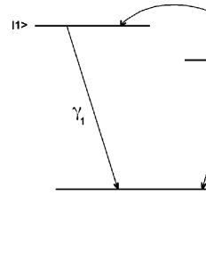
Figure 1: Three-level atom in the $V$ configuration (system I)

Time evolution of such system (which we call system I) is given by the master equation ficek

$$\frac{d\rho}{dt}=-i[H,\rho]+L_{I}\rho$$ (II.1)

where the damping term is

$$\begin{split}L_{I}\rho&=\frac{1}{2}\,\gamma_{1}(2\sigma_{31}\rho\sigma_{13}-\sigma_{11}\rho-\rho\sigma_{11})\\ &+\frac{1}{2}\,\gamma_{2}(2\sigma_{32}\rho\sigma_{23}-\sigma_{22}\rho-\rho\sigma_{22})\\ &+\frac{1}{2}\,\gamma_{12}(2\sigma_{31}\rho\sigma_{23}-\sigma_{21}\rho-\rho\sigma_{21})\\ &+\frac{1}{2}\,\gamma_{12}(2\sigma_{32}\rho\sigma_{13}-\sigma_{12}\rho-\rho\sigma_{12})\end{split}$$ (II.2)

In this equation, $\sigma_{jk}$ is the transition operator from $|{k}\rangle$ to $|{j}\rangle$ and $\gamma_{1},\,\gamma_{2}$ are spontaneous emission constants of $|{1}\rangle$ and $|{2}\rangle$ to the ground level $|{3}\rangle$. In addition

$$\gamma_{12}=\beta_{I}\sqrt{\gamma_{1}\gamma_{2}}$$ (II.3)

gives cross damping term between $|{1}\rangle\to|{3}\rangle$ and $|{2}\rangle\to|{3}\rangle$. The parameter $\beta_{I}$ represents the mutual orientation of transition dipole moments: when $\beta_{I}=1$, quantum interference is maximal and for $\beta_{I}=0$ it vanishes. Since we are mainly interested in the evolution of initial states due to the spontaneous emission, the form of the Hamiltonian $H$ is not discussed (see ficek for details).

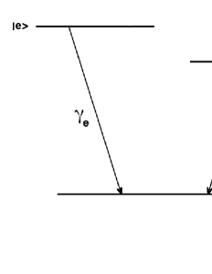
Figure 2: Three-level atom in the $V$ configuration (system II)

It is known that in atoms used in atomic spectroscopy, the transition dipole moments are usually perpendicular, so the system (I) described by equation (II.2) is difficult to realize. However, as was shown in Ref. ficek , the effects of quantum interference can be duplicated to a large degree by the three-level system (II) (FIG. 2) with exited states $|{e}\rangle,\,|{u}\rangle$ and the ground state $|{g}\rangle$, evolving according to the master equation with damping operator

$$\begin{split}L_{II}\rho&=\frac{1}{2}\gamma_{e}\,(2\sigma_{ge}\rho\sigma_{eg}-\sigma_{ee}\rho-\rho\sigma_{ee})\\ &+\frac{1}{2}\gamma_{u}\,(2\sigma_{gu}\rho\sigma_{ug}-\sigma_{uu}\rho-\rho\sigma_{uu})\end{split}$$ (II.4)

In the system (II), the dipole moments can be perpendicular and the measure of quantum interference is given by

$$\beta_{II}=\frac{\gamma_{e}-\gamma_{u}}{\gamma_{e}+\gamma_{u}}$$ (II.5)

So we can expect maximal effects of quantum interference in the system (II) when the level $|{u}\rangle$ is metastable.

III Entangled pair of three-level atoms

Now we consider a pair of three-level systems in the V configuration. In the context of evolution given by master equation generated by (II.2) or (II.4), we address the following question: how the dynamics of compound system of two atoms prepared initially in the entangled state is influenced by the presence of quantum interference? In particular, we may look at the time evolution of the appropriate measure of entanglement. Since damping causes that pure states evolve into mixed states, we need effective measure of mixed - state entanglement. As such measure one usually takes entanglement of formation $E_{F}(\rho)$ bennet , but in practice it is not known how to compute this measure for mixed states of pairs of $d$ - level systems in the case when $d>2$. A computable measure of entanglement was proposed in Ref. werner . It is based on the trace norm of the partial transposition $\rho^{T_{A}}$ of the state $\rho$. From the Peres’ criterion of separability peres , it follows that if $\rho^{T_{A}}$ is not positive, then $\rho$ is not separable. So one defines negativity of the state $\rho$ as

$$N(\rho)=\frac{||\rho^{T_{A}}||_{1}-1}{2}$$ (III.1)

$N(\rho)$ equals to the absolute value of the sum of negative eigenvalues of $\rho^{T_{A}}$ and is an entanglement monotone werner , but it can not detect bound entangled states horodecki .

The compound system of two atoms is defined on the space $\mathbb{C}^{3}\otimes\mathbb{C}^{3}$ and the matrix elements of the state $\rho$ will be considered with respect to the basis

$$\begin{split}\{&{\bm{e}}_{1}\otimes{\bm{e}}_{1},\,{\bm{e}}_{1}\otimes{\bm{e}}_{2},\,{\bm{e}}_{1}\otimes{\bm{e}}_{3},\,{\bm{e}}_{2}\otimes{\bm{e}}_{1},\,{\bm{e}}_{2}\otimes{\bm{e}}_{2},\,{\bm{e}}_{2}\otimes{\bm{e}}_{3},\\ &{\bm{e}}_{3}\otimes{\bm{e}}_{1},\,{\bm{e}}_{3}\otimes{\bm{e}}_{2},\,{\bm{e}}_{3}\otimes{\bm{e}}_{3}\}\end{split}$$ (III.2)

where $\{{\bm{e}}_{1},\,{\bm{e}}_{2},\,{\bm{e}}_{3}\}$ is the canonical basis of $\mathbb{C}^{3}$. In our discussion of entanglement evolution we focus on two classes of initial states. The first one consist of pure states of the form

$$\Psi_{\theta,\varphi}=\cos\theta\sin\varphi\,{\bm{e}}_{1}\otimes{\bm{e}}_{1}+\sin\theta\sin\varphi\,{\bm{e}}_{2}\otimes{\bm{e}}_{2}+\cos\varphi\,{\bm{e}}_{3}\otimes{\bm{e}}_{3}$$ (III.3)

where $\theta,\,\varphi\in[0,\pi/2]$. The states (III.3) have negativity

$$N(\Psi_{\theta,\varphi})=\cos\theta\sin\varphi\cos\varphi+\cos\theta\sin\theta\sin^{2}\varphi+\sin\theta\cos\varphi\sin\varphi$$ (III.4)

In the special case $\theta=\pi/4,\,\varphi=\arccos\frac{1}{\sqrt{3}}$, we obtain the state

$$\Psi_{\mathrm{max}}=\frac{1}{\sqrt{3}}\,({\bm{e}}_{1}\otimes{\bm{e}}_{1}+{\bm{e}}_{2}\otimes{\bm{e}}_{2}+{\bm{e}}_{3}\otimes{\bm{e}}_{3})$$ (III.5)

with maximal negativity $N(\Psi_{\mathrm{max}})=1$. The second class of so called isotropic mixed states hhh , is defined as follows: let

$$\rho_{0}=\frac{\openone_{9}}{9}$$

where $\openone_{9}$ is the identity matrix in $\mathbb{C}^{9}$, be the maximally mixed state of two three - level systems, then

$$W=(1-p)\,\rho_{0}+p\,|{\Psi_{\mathrm{max}}}\rangle\langle{\Psi_{\mathrm{max}}}|,\quad p\in[0,1]$$ (III.6)

interpolate between maximally entangled and maximally mixed states. Notice that states (III.6) are the natural generalizations of Werner states wer of two-qubit systems. One can check that negativity of (III.6) equals

$$N(W)=\begin{cases}0,&p\leq\frac{1}{4}\\ \frac{1}{3}\,(4p-1),&p>\frac{1}{4}\end{cases}$$ (III.7)

IV Time evolution of negativity

Consider first the system of two distant three - level atoms $A$ and $B$ , both of type (II). This case is simpler to analyse and can be solved exactly. Since the atoms are independent and do not interact, the dissipative part of dynamics is given by the master equation

$$\frac{d\rho}{dt}=L_{\mathrm{II}}^{AB}\rho$$ (IV.1)

with

$$\begin{split}L_{II}^{AB}\rho&=\frac{1}{2}\gamma_{e}\,(2\sigma_{ge}^{A}\rho\sigma_{eg}^{A}-\sigma_{ee}^{A}\rho-\rho\sigma_{ee}^{A})\\ &+\frac{1}{2}\gamma_{u}\,(2\sigma_{gu}^{A}\rho\sigma_{ug}^{A}-\sigma_{uu}^{A}\rho-\rho\sigma_{uu}^{A})\\ &+\frac{1}{2}\gamma_{e}\,(2\sigma_{ge}^{B}\rho\sigma_{eg}^{B}-\sigma_{ee}^{B}\rho-\rho\sigma_{ee}^{B})\\ &+\frac{1}{2}\gamma_{u}\,(2\sigma_{gu}^{B}\rho\sigma_{ug}^{B}-\sigma_{uu}^{B}\rho-\rho\sigma_{uu}^{B})\end{split}$$ (IV.2)

where

$$\sigma_{kl}^{A}=\sigma_{kl}\otimes\openone_{3},\quad\sigma_{kl}^{B}=\openone_{3}\otimes\sigma_{kl},\quad k,l=e,u,g$$

Moreover, we identify the states $|{e}\rangle,\,|{u}\rangle$ and $|{g}\rangle$ with vectors ${\bm{e}}_{1},\,{\bm{e}}_{2}$ and ${\bm{e}}_{3}$ respectively. The master equation (IV.1) can be used to obtain the equations for matrix elements of any density matrix of compound system, with respect to the basis (III.2). The calculations are tedious but elementary, so we are not discussing details. As a result, we obtain the following properties of dynamics given by (IV.1):

1. for $\gamma_{u}>0$, the dynamics brings all initial states into unique asymptotic state $|{g}\rangle\otimes|{g}\rangle$,

2. in the case of maximal interference ($\gamma_{u}=0$), the dynamics is not ergodic, and asymptotic stationary states $\rho_{\mathrm{as}}$ depend on initial conditions.

The case of maximal interference will be studied in the next section, now we discuss the evolution of entanglement in the first case. Since the asymptotic state is separable, negativity of any initially entangled state goes to zero with time. To see some details, consider initial states of the form

$$\rho=\begin{pmatrix}\rho_{11}&\cdots&\rho_{15}&\cdots&\rho_{19}\\ \vdots&&\vdots&&\vdots\\ \rho_{51}&\cdots&\rho_{55}&\cdots&\rho_{59}\\ \vdots&&\vdots&&\vdots\\ \rho_{91}&\cdots&\rho_{95}&\cdots&\rho_{99}\end{pmatrix}$$ (IV.3)

Notice that pure states (III.3) are particular examples of (IV.3). The solution $\rho(t)$ of master equation (IV.1) for initial condition (IV.3) has matrix elements

$$\begin{split}\rho_{11}(t)&=e^{-2\gamma_{e}t}\,\rho_{11}\\ \rho_{15}(t)&=e^{-(\gamma_{e}+\gamma_{u})t}\,\rho_{15}\\ \rho_{19}(t)&=e^{-\gamma_{e}t}\,\rho_{19}\\ \rho_{33}(t)&=(e^{-\gamma_{e}t}-e^{-2\gamma_{e}t})\,\rho_{11}\\ \rho_{55}(t)&=e^{-2\gamma_{e}t}\,\rho_{55}\\ \rho_{59}(t)&=e^{-\gamma_{u}t}\,\rho_{59}\\ \rho_{66}(t)&=(e^{-\gamma_{u}t}-e^{-2\gamma_{u}t})\,\rho_{55}\\ \rho_{77}(t)&=(e^{-\gamma_{e}t}-e^{-2\gamma_{e}t})\,\rho_{11}\\ \rho_{88}(t)&=(e^{-\gamma_{u}t}-e^{-2\gamma_{u}t})\,\rho_{55}\\ \rho_{99}(t)&=(1+e^{-2\gamma_{e}t}-2e^{-\gamma_{e}t})\,\rho_{11}\\ &+(1+e^{-2\gamma_{u}t}-2e^{-\gamma_{u}t})\,\rho_{55}+\rho_{99}\end{split}$$ (IV.4)

where for remaining matrix elements one can use hermiticity of $\rho(t)$. Even in that case, the analytic formula for negativity as a function of time is rather involved, so we consider explicit example. Take as initial state $\Psi_{\mathrm{max}}$ which is maximally entangled, then

$$N_{\Psi_{\mathrm{max}}}(t)=\frac{1}{3}\left(e^{-2\gamma_{e}t}+e^{-(\gamma_{e}+\gamma_{u})t}+e^{-2\gamma_{u}t}\right)$$ (IV.5)

Figure 3: Time-dependence of negativity for initial state $\Psi_{\mathrm{max}}$ for different values of $\alpha=\gamma_{u}/\gamma_{e}$

Observe that (IV.5) vanishes asymptotically at the rate depending on degree of interference: the larger is the effect of interference, the slower is the process of disentanglement (FIG. 3). Notice also that in the limit of maximal interference ($\gamma_{u}\to 0$), some part of initial entanglement can survive. One can also check that other entangled states from the class (III.3) behave similarly (see FIG. 4).

Figure 4: Time-dependence of negativity for initial state (III.3) with $\theta=\pi/8,\,\varphi=\pi/6$ and different values of $\alpha=\gamma_{u}/\gamma_{e}$

Figure 5: Time-dependence of negativity for initial state $W$ with $p=3/4$ and different values of $\alpha=\gamma_{u}/\gamma_{e}$

When the initial state is mixed isotropic state $W$ given by (III.6), then $W(t)$ has matrix elements

$$\begin{split}W_{11}(t)&=\frac{1}{9}(1+2p)\,e^{-2\gamma_{e}t}\\ W_{15}(t)&=\frac{1}{3}p\,e^{-(\gamma_{e}+\gamma_{u})t}\\ W_{19}(t)&=\frac{1}{3}p\,e^{-\gamma_{e}t}\\ W_{22}(t)&=\frac{1}{9}(1-p)\,e^{-(\gamma_{e}+\gamma_{u})t}\\ W_{33}(t)&=\frac{1}{9}(p-1)\,e^{-(\gamma_{e}+\gamma_{u})t}-\frac{1}{9}(1+2p)\,e^{-2\gamma_{e}t}+\frac{1}{3}\,e^{-\gamma_{e}t}\\ W_{44}(t)&=\frac{1}{9}(1-p)\,e^{-(\gamma_{e}+\gamma_{u})t}\\ W_{55}(t)&=\frac{1}{9}(1+2p)\,e^{-2\gamma_{u}t}\\ W_{59}(t)&=\frac{1}{3}p\,e^{-\gamma_{u}t}\\ W_{66}(t)&=\frac{1}{9}(p-1)\,e^{-(\gamma_{e}+\gamma_{u})t}-\frac{1}{9}(1+2p)\,e^{-2\gamma_{u}t}+\frac{1}{3}\,e^{-\gamma_{u}t}\\ W_{77}(t)&=W_{33}(t)\\ W_{88}(t)&=W_{66}(t)\\ W_{99}(t)&=1+\frac{1}{9}(1+2p)\,(e^{-2\gamma_{e}t}+e^{-2\gamma_{u}t})+\frac{2}{9}(1-p)\,e^{-(\gamma_{e}+\gamma_{u})t}\\ &-\frac{2}{3}\,(e^{-\gamma_{e}t}+e^{-\gamma_{u}t})\end{split}$$ (IV.6)

Explicit formula for negativity of $W(t)$ is lengthy and involved, so we not reproduce it here. But it follows from the calculations, that the time dependence of negativity is similar to the case of pure states (FIG. 5).

V Maximal interference and asymptotic entanglement

The case of maximal interference in system (II) can be discussed in details. Take any initial state $\rho$ with matrix elements $\rho_{ij}$. The dynamics given by the master equation (IV.1) has a remarkable property: in the case of maximal interference between transitions $|{e}\rangle\to|{g}\rangle$ and $|{u}\rangle\to|{g}\rangle$, there are nontrivial stationary asymptotic states $\rho_{\mathrm{as}}$. By a direct calculations, one can show that $\rho_{\mathrm{as}}$ have the following non-vanishing matrix elements

$$\begin{split}&(\rho_{\mathrm{as}})_{55}=\rho_{55},\quad(\rho_{\mathrm{as}})_{56}=\rho_{56},\quad(\rho_{\mathrm{as}})_{58}=\rho_{58},\quad\\ &(\rho_{\mathrm{as}})_{59}=\rho_{59},\quad(\rho_{\mathrm{as}})_{68}=\rho_{68},\quad(\rho_{\mathrm{as}})_{66}=\rho_{44}+\rho_{66}\\ &(\rho_{\mathrm{as}})_{69}=\rho_{47}+\rho_{69},\quad(\rho_{\mathrm{as}})_{88}=\rho_{22}+\rho_{88}\\ &(\rho_{\mathrm{as}})_{89}=\rho_{23}+\rho_{89},\quad(\rho_{\mathrm{as}})_{99}=\rho_{11}+\rho_{33}+\rho_{77}+\rho_{99}\end{split}$$ (V.1)

It is very interesting that although two atoms are independent and do not interact, some of these asymptotic states can be entangled. Quantum interference causes that part of initial entanglement can survive the process of decoherence. For example, if initial states are pure states (III.3), then $\rho_{\mathrm{as}}$ has only four nonvanishing matrix elements

$$\begin{split}&(\rho_{\mathrm{as}})_{55}=\sin^{2}\varphi\sin^{2}\theta,\quad(\rho_{\mathrm{as}})_{59}=\cos\varphi\sin\varphi\sin\theta,\\ &(\rho_{\mathrm{as}})_{99}=\cos^{2}\varphi+\sin^{2}\varphi\cos^{2}\theta\end{split}$$ (V.2)

and

$$N(\rho_{\mathrm{as}})=\sin\varphi\cos\varphi\sin\theta$$ (V.3)

Comparing (III.4) with (V.3) we see that

$$N(\rho_{\mathrm{as}})\leq N(\Psi_{\theta,\varphi})$$

Consider now some special cases:
1. Let $\theta=\pi/4$ then

$$\widetilde{\Psi}_{\varphi}=\frac{\sin\varphi}{\sqrt{2}}\,({\bm{e}}_{1}\otimes{\bm{e}}_{1}+{\bm{e}}_{2}\otimes{\bm{e}}_{2})+\cos\varphi{\bm{e}}_{3}\otimes{\bm{e}}_{3}$$

where $0<\varphi<\pi/2$. The states $\widetilde{\Psi}_{\varphi}$ have negativity

$$N(\widetilde{\Psi}_{\varphi})=\frac{1}{2}\sin\varphi(2\sqrt{2}\cos\varphi+\sin\varphi)$$

and

$$N(\rho_{\mathrm{as}})=\frac{\sin\varphi\,\cos\varphi}{\sqrt{2}}$$

which is always greater then zero.
2. Let $\theta=\pm\pi/2,\,\varphi\in(0,\pi/2)$, then the states

$$\Psi_{\varphi}^{\pm}=\pm\sin\varphi\,{\bm{e}}_{2}\otimes{\bm{e}}_{2}+\cos\varphi\,{\bm{e}}_{3}\otimes{\bm{e}}_{3}$$

are stable during the evolution, and

$$N(\rho_{\mathrm{as}})=N(\Psi_{\varphi}^{\pm})=\cos\varphi\,\sin\varphi$$

3. Let $\theta=0$, then the states

$$\Psi_{\varphi}^{0}=\sin\varphi\,{\bm{e}}_{1}\otimes{\bm{e}}_{1}+\cos\varphi\,{\bm{e}}_{3}\otimes{\bm{e}}_{3},\quad\varphi\in(0,\pi/2)$$

are entangled with negativity $N(\Psi_{\varphi}^{0})=\sin\varphi\,\cos\varphi$, but $\rho_{\mathrm{as}}={\bm{e}}_{3}\otimes{\bm{e}}_{3}$ is separable.
When the initial state is the isotropic $W$, then the nonvanishing matrix elements of $W_{\mathrm{as}}$ are

$$\begin{split}&(W_{\mathrm{as}})_{55}=\frac{1}{9}\,(1+2p),\quad(W_{\mathrm{as}})_{59}+\frac{p}{3}\\ &(W_{\mathrm{as}})_{66}=\frac{2}{9}\,(1-p),\quad(W_{\mathrm{as}})_{88}=\frac{2}{9}\,(1-p)\\ &(W_{\mathrm{as}})_{99}=\frac{2(2+p)}{9}\end{split}$$ (V.4)

and

$$N(W_{\mathrm{as}})=\begin{cases}0,&p\leq\frac{2}{5}\\ \frac{1}{9}\,(5p-2),&p>\frac{2}{5}\end{cases}$$ (V.5)

So for $p>\frac{2}{5}$, asymptotic states are still entangled.

VI System of atoms of type (I). Numerical results

When we consider two atoms of type (I), the analysis of evolution of the system is much more involved. For distant atoms the master equation reads

$$\frac{d\rho}{dt}=L_{I}^{AB}\rho$$ (VI.1)

with

$$\begin{split}L_{I}^{AB}\rho&=\frac{1}{2}\,\gamma_{1}(2\sigma_{31}^{A}\rho\sigma_{13}^{A}-\sigma_{11}^{A}\rho-\rho\sigma_{11}^{A})\\ &+\frac{1}{2}\,\gamma_{2}(2\sigma_{32}^{A}\rho\sigma_{23}^{A}-\sigma_{22}^{A}\rho-\rho\sigma_{22}^{A})\\ &+\frac{1}{2}\,\gamma_{12}(2\sigma_{31}^{A}\rho\sigma_{23}^{A}-\sigma_{21}^{A}\rho-\rho\sigma_{21}^{A})\\ &+\frac{1}{2}\,\gamma_{12}(2\sigma_{32}^{A}\rho\sigma_{13}^{A}-\sigma_{12}^{A}\rho-\rho\sigma_{12}^{A})\\ &+\frac{1}{2}\,\gamma_{1}(2\sigma_{31}^{B}\rho\sigma_{13}^{B}-\sigma_{11}^{B}\rho-\rho\sigma_{11}^{B})\\ &+\frac{1}{2}\,\gamma_{2}(2\sigma_{32}^{B}\rho\sigma_{23}^{B}-\sigma_{22}^{B}\rho-\rho\sigma_{22}^{B})\\ &+\frac{1}{2}\,\gamma_{12}(2\sigma_{31}^{B}\rho\sigma_{23}^{B}-\sigma_{21}^{B}\rho-\rho\sigma_{21}^{B})\\ &+\frac{1}{2}\,\gamma_{12}(2\sigma_{32}^{B}\rho\sigma_{13}^{B}-\sigma_{12}^{B}\rho-\rho\sigma_{12}^{B})\end{split}$$ (VI.2)

where $\sigma_{kl}^{A},\,\sigma_{kl}^{B}$ for $k,l=1,2,3$ are defined as in Sect. IV. Notice that in the present section, the vectors ${\bm{e}}_{1},\,{\bm{e}}_{2}$ and ${\bm{e}}_{3}$ represent states $|{1}\rangle,\,|{2}\rangle$ and $|{3}\rangle$ respectively and cross damping rate $\gamma_{12}$ is given by (II.3).

Figure 6: Time-dependence of negativity for pure initial state (III.3) with $\varphi=\pi/6,\,\theta=\pi/8$, for $\gamma_{2}/\gamma_{1}=0.9$ and different values of $\beta_{I}$

Figure 7: Time-dependence of negativity for isotropic initial state (III.6) with $p=3/4$, for $\gamma_{2}/\gamma_{1}=0.9$ and different values of $\beta_{I}$

From (VI.1) we obtain a system of differential equations for matrix elements of density matrix $\rho$ which we solve numerically. The results can be used to analyse time evolution of negativity of given initial state. Since in a single three-level atom the effect of quantum interference can be observed in both systems (I) and (II) ficek , we expect that also in this model the presence of interference will slow down the process of disentanglement.

Figure 8: Time-dependence of negativity for initial state (III.5) in the case of maximal interference and for different values of $\kappa=\gamma_{2}/\gamma_{1}$

Numerical results entirely confirm these expectations. In particular, we show that when $\beta_{I}<1$, all initial states evolve to the asymptotic state $|{{\bm{e}}_{3}}\rangle\langle{{\bm{e}}_{3}}|$, so disentangle asymptotically, but as in the previous case, the rate of disentanglement depends on quantum interference: for larger $\beta_{I}$ the process of disentanglement is slower. FIGS. 6 and 7 represent the results of calculations for pure initial state (III.3) with $\varphi=\pi/6,\,\theta=\pi/8$ and isotropic state (III.6) with $p=3/4$.

In the case of maximal interference ($\beta_{I}=1$), we also observe that the system has nontrivial asymptotic states with non-zero negativity. For example, FIG. 8 represents the results of numerical calculations of evolution of negativity for maximally entangled initial state (III.5).

VII Conclusions

We have studied dynamical aspects of entanglement in a system ot two independent three-level atoms in $V$-configuration, interacting with the vacuum. Spontaneous emission causes decoherence and degradation of initial entanglement, but quantum interference between principal transition in each atom can slow down the process of disentanglement. We have shown this effect using two models of dynamics, which at the level of single three-level atom predict the phenomenon of interference. Our results indicate that these two kinds of quantum evolutions similarly describe dynamical behaviour of entanglement in the system.

References

• (1) W. K. Wooters, Phys. Rev. Lett. 80, 2245(1998).
• (2) T. Yu, J.H. Eberly, Phys. Rev. Lett. 93, 140404(2004).
• (3) P.J. Dodd, Phys. Rev. A69, 052106(2004).
• (4) A. Jamróz, J. Phys. A 39, 7727(2006).
• (5) L. Jakóbczyk, A. Jamróz, Phys. Lett. A333, 35(2004).
• (6) A. Peres, Phys. Rev. Lett. 77, 1413(1996).
• (7) P. Horodecki, Phys. Lett. A 232, 333(1997).
• (8) G.S. Agarwal, Quantum Statistical Properties of Spontaneous Emission and their Relation to Other Approaches, Springer, Berlin, 1974.
• (9) Z. Ficek, S. Swain, Phys. Rev. A 69, 023401(2004).
• (10) G.H. Hegerfeld, M. B. Plenio, Phys. Rev. A 46, 373(1992).
• (11) P. Zoller, M. Marte, D.F. Walls, Phys. Rev. A 35, 198(1987).
• (12) P. Zhou, S. Swain, Phys. Rev. Lett. 77, 3995(1996).
• (13) S.E. Harris, Phys. Rev. Lett. 62, 1033(1989).
• (14) C.H. Bennet, D.P. DiVincenzo, J.A. Smolin, W.K. Wootters, Phys. Rev. A 54, 3824(1996).
• (15) G. Vidal, R.F. Werner, Phys. Rev. A 65, 032314(2002).
• (16) M. Horodecki, P. Horodecki, R. Horodecki, Phys. Rev. A textb60, 1888(1999).
• (17) R.F. Werner, Phys. Rev. A 40, 4277(1989).