Cantilever cooling with radio frequency circuits

Abstract

We consider a method to reduce the kinetic energy in a low-order mode of a miniature cantilever. If the cantilever contributes to the capacitance of a driven RF circuit, a force on the cantilever exists due to the electric field energy stored in the capacitance. If this force acts with an appropriate phase shift relative to the motion of the cantilever, it can oppose the velocity of the cantilever, leading to cooling. Such cooling may enable reaching the quantum regime of cantilever motion.

Precise control of quantum systems occupies the efforts of many laboratories; an important recent application of such control is in quantum information processing. Some of this work is devoted to controlling the motion of a mechanical oscillator at the quantum level. This has already been accomplished in a “bottom-up” approach where a single atom is confined in a harmonic well. For example, it has been possible to make nonclassical mechanical oscillator states such as squeezed, Fock, and Schrödinger-cat states meekhof96 ; monroe96_cats . However, for various applications, there is also interest in a “top-down” strategy, which has approached the quantum limit by using smaller and smaller micro-mechanical resonators (for a summary, see e.g., schwab05 ). In this case, small ($\sim 1~{}\mu$m) mechanical resonators, having low-order mode frequencies of approximately 10 - 100 MHz, can approach the quantum regime at low temperature ($<$ 1 K); mean thermal occupation numbers of approximately 50 have been achieved lahaye04 .

To reach the quantum level of a mechanical oscillator, an efficient cooling mechanism is desirable. With harmonically bound atoms, this can be achieved with laser cooling where, in a room temperature apparatus, the modes of mechanical motion can be cooled to a level where the occupation numbers $\langle n\rangle$ of the quantized modes reach values less than 0.1 for oscillation frequencies $\sim 1-10$ MHz diedrich89 ; monroe_cooling . For more macroscopic mechanical oscillators, other means are sought. An extension of laser cooling of atoms would be to couple laser cooled atomic ions to a (charged) macroscopic oscillator heinzen90 ; bible ; tian04 ; hensinger05 ; here, the macroscopic oscillator would be cooled sympathetically through its Coulomb coupling to the ions. Analogously, the resonator might be cooled by coupling to other quantum systems wilson-rae04 ; martin04 ; zhang05 ; blencowe05 ; clerk05 .

Cooling of a macroscopic mechanical oscillator can also be achieved by feedback applied with optical forces. The feedback can be obtained using external electronics to control radiation pressure as in cohadon99 . In metzger04 , the authors describe several passive means of optical feedback. Their experiment reported cooling by means of photothermal forces, but they also describe theoretically passive-feedback cooling by means of the radiation pressure force. In this note we describe (classically) a related possible cooling mechanism where the cooling force is between capacitor plates that contain a radio frequency (RF) electric field.

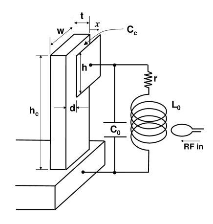
Figure 1: Cantilever and associated RF circuitry. We assume the cantilever is approximated by a thin beam fixed to a rigid base at one end (lower left). The plate of area w$\cdot$h attached to the RF circuit is also assumed to be mechanically rigid.

To describe the cooling mechanism, we refer to the simplified situation shown in Fig. 1. We assume a conducting beam cantilever, having density $\rho$, which is fixed rigidly at one end. One face of the cantilever is placed a distance d from a rigidly mounted plate of area w$\cdot$h thereby forming a parallel-plate capacitor $\mathrm{C_{c}}=\epsilon_{0}$w$\cdot$h/d where $\epsilon_{0}$ is the vacuum dielectric constant. An inductor L₀ and capacitor C₀ are connected in parallel with $\mathrm{C_{c}}$ to form a parallel tank circuit with (RF) resonant frequency $\Omega_{0}=1/\sqrt{\mathrm{L_{0}(C_{0}+C_{c})}}$. For simplicity, we assume all losses in the RF circuit (including the coupling to the source impedance) are represented by a resistance r. We also assume $Q_{\mathrm{RF}}=\Omega_{0}\mathrm{L_{0}/r}\gg 1$ where $Q_{\mathrm{RF}}$ is the quality factor of the RF circuit.

For simplicity, we consider only the lowest-order bending mode of the cantilever, where the free end oscillates back and forth (in the $\hat{x}$ direction in Fig. 1) with frequency $\omega_{c}$, which we assume to be much smaller than $\Omega_{0}$. Small displacements $x$ of the cantilever can be described by the equation of motion

$$m\ddot{x}+m\Gamma\dot{x}+m\omega_{c}^{2}x=F,$$ (1)

where $\Gamma$ is the damping rate of the cantilever oscillation, $F$ is the force on the end of the cantilever, and $m$ is the effective mass of the cantilever, given by $\rho\mathrm{wh_{0}t/4}$ sidles95 . The force $F$ includes random thermal forces as well as purposely applied forces.

If a potential V is applied to capacitor $\mathrm{C_{c}}$, the capacitor plates experience a mutual attractive force; in the context of Fig. 1, the cantilever feels a force $F_{\mathrm{E}}=\epsilon_{0}\mathrm{E^{2}wh}/2=\mathrm{C_{c}V^{2}/(2d)}$ in the positive $x$ direction, where E = V/d is the electric field between the capacitor plates. Here we will be interested in the case where V is an applied RF potential $\mathrm{V_{RF}\cos\Omega_{\mathrm{RF}}t}$ with $\Omega_{\mathrm{RF}}\simeq\Omega_{0}$. Since $\omega_{c}\ll\Omega_{0}$, the force for frequencies around $\omega_{c}$ is given by the averaged RF force

$$F_{\mathrm{E}}=\frac{\mathrm{C_{c}}\langle\mathrm{V^{2}}\rangle}{2\mathrm{d}}=\mathrm{\frac{C_{c}V_{RF}^{2}}{4d}}=\frac{\epsilon_{0}\mathrm{whV_{RF}^{2}}}{\mathrm{4d^{2}}}.$$ (2)

This RF capacitive force will give rise to the cooling as follows. As the cantilever oscillates back and forth, its motion modulates the overall capacitance of the RF circuit ($\mathrm{C_{c}+C_{0}}$) thereby modulating the RF circuit’s resonant frequency. If the input RF frequency is tuned to the lower side of the RF resonance, as the frequency of the circuit is modulated, so too is the RF electric field amplitude in the capacitance of the circuit. As described below, this gives rise to an additional oscillating capacitive force term that will shift the resonant frequency of the cantilever. However, due to the finite response time of the RF circuit (given by $Q_{\mathrm{RF}}$), there is a phase lag in this additional capacitive force term relative to the cantilever motion. This phase lag leads to a force component that opposes the velocity of the cantilever, thereby leading to the cooling.

The average RF capacitive force will displace the equilibrium position of the cantilever. However, we will be mainly interested in small deviations of the cantilever around its equilibrium position $\mathrm{d_{0}}$; therefore, for the moment, we will assume this displacement is absorbed into the definition of $\mathrm{d_{0}}$ and write d $\equiv\mathrm{d_{0}}-x$ . For small deviations $x$ around the equilibrium position, we write

$$\delta F_{\mathrm{E}}=(\partial F_{\mathrm{E}}/\partial x)x.$$ (3)

To evaluate this expression, we note that $F_{\mathrm{E}}$ depends on $x$ through d as well as through $\mathrm{V_{RF}}$,

$$\frac{\partial F_{\mathrm{E}}}{\partial x}=\frac{\epsilon_{0}\mathrm{wh}}{4}\biggl{[}\mathrm{V_{RF}^{2}}\frac{\partial\mathrm{(1/d^{2})}}{\partial x}+\frac{1}{\mathrm{d^{2}}}\frac{\partial\mathrm{V_{RF}^{2}}}{\partial x}\biggr{]}.$$ (4)

This is because as $x$ changes, $\mathrm{C_{c}}$ changes thereby changing $\Omega_{0}$. If RF is applied to the circuit of Fig. 1 at a frequency $\Omega$ near $\Omega_{0}$, $\mathrm{V_{RF}}$ will depend on $x$ due to its dependence on $\Omega-\Omega_{0}$.

Here, we will assume that the RF frequency modulation caused by the cantilever is less than than the bandwidth $\Omega_{0}/Q_{\mathrm{RF}}$ of the RF circuit. In this case we can write

$$\frac{\partial\mathrm{V_{RF}^{2}}}{\partial x}\simeq\frac{\partial\mathrm{V_{RF}^{2}}}{\partial\Omega_{0}}\cdot\frac{\partial\Omega_{0}}{\partial\mathrm{C_{c}}}\cdot\frac{\partial\mathrm{C_{c}}}{\partial x}\ .$$ (5)

The first factor on the right-hand-side of this equation can be obtained from the expression for the RF potential across the circuit of Fig. 1 relative to the maximum (on-resonance) RF potential $\mathrm{V_{max}}$ for a fixed input power

$$\mathrm{\frac{V_{RF}^{2}}{V_{max}^{2}}}\simeq\frac{1}{1+\bigl{[}2Q_{\mathrm{RF}}\frac{\Omega_{\mathrm{RF}}-\Omega_{0}}{\Omega_{0}}\bigr{]}^{2}}\ .$$ (6)

When the input RF frequency is tuned to the “half-power” points of the RF circuit ($2Q_{\mathrm{RF}}(\Omega_{\mathrm{RF}}-\Omega_{0})/\Omega_{0}=\pm 1$), we find $\partial\mathrm{(V_{RF}^{2}/V_{max}^{2})}/\partial\Omega_{0}=\pm Q/\Omega_{0}$.

The second and third factors in Eq. (5) are $\partial\Omega_{0}/\partial\mathrm{C_{c}}=-\Omega_{0}/(2\mathrm{(C_{0}+C_{c})})$ and $\partial\mathrm{C_{c}}/\partial x=\mathrm{C_{c}/d_{0}}$. With these expressions, Eq. (5) at the half-power points becomes

$$\frac{\partial\mathrm{V_{RF}^{2}}}{\partial x}=\pm\mathrm{V_{max}^{2}}\frac{Q_{\mathrm{RF}}}{2\mathrm{d_{0}}}\frac{\mathrm{C_{c}}}{\mathrm{C_{c}+C_{0}}},$$ (7)

where the $+~{}(-)$ sign refers to $\Omega_{\mathrm{RF}}<(>)\ \Omega_{0}$. This dependence of the capacitor plate force with cantilever position is analogous to the dependence of the radiation pressure force on the mirrors in an optical cavity with the spacing of the cavity mirrors metzger04 .

Combining these expressions, Eq. (4) becomes

$$\delta F_{\mathrm{E}}=\mathrm{\frac{C_{c}V_{max}^{2}}{4d_{0}^{2}}}\biggl{[}1\pm\frac{Q_{\mathrm{RF}}}{2}\mathrm{\frac{C_{c}}{C_{c}+C_{0}}}\biggr{]}x.$$ (8)

When substituted into the right-hand side of Eq. (1), this expression only alters the spring constant $m\omega_{c}^{2}$ and therefore the oscillation frequency of the cantilever. However, Eq. (7) gives the change of $\mathrm{V_{RF}^{2}}$ vs. $x$ assuming that the RF energy has reached its steady-state value. In fact, as $x$ changes, $\mathrm{V_{RF}^{2}}$ requires a time $\tau$ to reach its steady state value, where $\tau$ is the decay time of the RF circuit.

This lag in time is analogous to how the output voltage $\mathrm{V_{out}}$ following a low-pass RC filter changes in response to changes in the input voltage $\mathrm{V_{in}}$. For this case, the output voltage responds to input signals $\mathrm{V_{in}=|V_{in}}|e^{i\omega t}$ with a transfer function

$$\mathrm{V_{out}/V_{in}}=\cos{\phi}\ e^{-i\phi},$$ (9)

where $\phi\equiv\tan^{-1}(\omega\tau)$ and $\tau=$ RC.

Analogously, a similar transfer function must be applied to Eq. (7) and the second term in Eq. (8), assuming $x\rightarrow x_{0}e^{i\omega t}$. With this modification, Eq. (8) becomes

$$\delta F_{\mathrm{E}}=\mathrm{\frac{C_{c}V_{max}^{2}}{4d_{0}^{2}}}\biggl{[}1\pm\cos{\phi}e^{-i\phi}\frac{Q_{\mathrm{RF}}}{2}\mathrm{\frac{C_{c}}{C_{c}+C_{0}}}\biggr{]}x,$$ (10)

where $\omega$ is the cantilever frequency and $\tau$ is now the decay time of the RF circuit. Noting that $ix=\dot{x}/\omega$, Eq. (1) with the force $F=\delta F_{\mathrm{E}}+F_{0}e^{i\omega t}$ becomes

$$m\ddot{x}+m(\Gamma+\Gamma^{\prime})\dot{x}+m\omega_{c}^{2}(1-\kappa)x=F_{0}e^{i\omega t},$$ (11)

where

$$\kappa\equiv\frac{\mathrm{C_{c}V_{max}^{2}}}{4m\omega_{c}^{2}\mathrm{d_{0}^{2}}}\biggl{[}1\pm\frac{\cos^{2}{\phi}\ Q_{\mathrm{RF}}\mathrm{C_{c}}}{\mathrm{2(C_{c}+C_{0})}}\biggr{]},$$ (12)

$$\Gamma^{\prime}\equiv\pm\frac{Q_{\mathrm{RF}}\mathrm{V_{max}^{2}C_{c}^{2}}}{16m\omega_{c}\mathrm{d_{0}^{2}(C_{c}+C_{0})}}\sin{2\phi},$$ (13)

and the $\pm$ sign conventions are as noted above. The term $\kappa$ results in a frequency shift of the cantilever mode. For $\Omega_{\mathrm{RF}}<\Omega_{0}$ the term $\Gamma^{\prime}$ gives rise to an increased damping and will lead to cooling.

Before considering cooling, we must first examine the sources of noise in the system. Assuming the cantilever is at temperature $T$, the spectral density of force fluctuations acting on the isolated cantilever at frequencies near $\omega_{c}$ is given by sidles95 .

$$S_{F}(\mathrm{CANT})=4k_{B}Tm\omega_{c}/Q_{c}=4k_{B}Tm/\tau_{c},$$ (14)

where $k_{B}$ is Boltzmann’s constant, and $Q_{c}$ and $\tau_{c}$ are the cantilever $Q$-factor and (energy) decay time constant.

We must also consider noise in the RF circuit and its effect on the cantilever. In Eq. (2), we need to replace $\mathrm{V_{RF}}$ with $\mathrm{V_{RF}}+v_{n}(\mathrm{C_{c}})$, where $v_{n}(\mathrm{C_{c}})$ is the Johnson noise potential (characterized by noise spectral density $S_{v_{n}}(\mathrm{C_{c}})$)) across the cantilever capacitance $\mathrm{C_{c}}$ due to resistance in the RF circuit. In particular, the cantilever will be affected by RF noise at frequencies near $\Omega_{\mathrm{RF}}\pm\omega_{c}$ because cross terms in Eq. (2) will give rise to random forces at the cantilever frequency. (Here we assume the RF modulation index due to cantilever motion is much less than one, which will be true for the examples below.) The voltage noise spectral density from the resistor $r$ in Fig. 1 is given by $S_{v_{n}}(r)=4k_{B}Tr$. From an analysis of the circuit we can then calculate $S_{v_{n}}(\mathrm{C_{c}})$. With this and Eq. (2), we find the spectral density of force fluctuations due the RF circuit noise to be

$$S_{F}(RF)=\frac{1}{2}\biggl{[}\mathrm{\frac{C_{c}V_{RF}}{d_{0}}}\biggr{]}^{2}S_{v_{n}}(\mathrm{C_{c}}).$$ (15)

In general, we must also consider other sources of noise, such as that from a detection circuit that is connected to the circuit in Fig. 1. Depending on the detection method used, this noise can be important; however, for simplicity, we assume the detection can be switched on and off without significantly affecting the energy of the cantilever.

Considering only $S_{F}(\mathrm{CANT})$ and $S_{F}(\mathrm{RF})$, the effective temperature of the mode that is acted on is increased by the additional noise from the RF circuit, but lowered by the increased damping

$$\frac{T_{\mathrm{eff}}}{T}=\biggl{[}\frac{\Gamma}{\Gamma+\Gamma^{\prime}}\biggr{]}\biggl{[}\frac{S_{F}(\mathrm{RF})+S_{F}(\mathrm{CANT})}{S_{F}(\mathrm{CANT})}\biggr{]}.$$ (16)

To get an approximate idea of the cooling that might be achieved, we first consider a silicon cantilever where the doping is high enough that we can neglect heating from RF currents. We assume $\mathrm{h_{c}}=1.5$ mm, $\mathrm{h}=0.5$ mm, $\mathrm{t}=20\ \mu$m, $\mathrm{w}=400\ \mu$m, $\mathrm{d_{0}}=10\ \mu$m. The frequency of the lowest-order bending mode is given by sidles95

$$\omega_{\mathrm{c}}=3.516\mathrm{\frac{t}{h_{\mathrm{c}}^{2}}}\sqrt{\frac{E}{12\rho}},$$ (17)

where $E=1.07\times 10^{11}$ Pa and $\rho=2.33\times 10^{3}\ \mathrm{kg/m}^{2}$ are the Young’s modulus and density of silicon. For these parameters we find $\omega_{\mathrm{c}}/2\pi=9.73$ kHz, $m=7.00\times 10^{-9}$ kg, and $\mathrm{C_{c}}=0.177$ pF. We assume $\tau_{\mathrm{c}}=5$ s.

For the RF circuit we assume $\Omega_{\mathrm{RF}}/2\pi=50$ MHz, $\mathrm{C_{0}}=10$ pF, $Q_{\mathrm{RF}}=400$. With $\mathrm{V_{max}}=20$ V, we find $S_{F}(\mathrm{RF})/S_{F}(\mathrm{CANT})=1.40$, $\kappa=0.0302$, $\Gamma^{\prime}/\Gamma=558$, and $T_{\mathrm{eff}}/T=4.30\times 10^{-3}$. For this example, the final mean occupation number $\langle n\rangle$ of the fundamental mode of cantilever is $>10^{6}$ for T = 300 K. Assuming the cantilever spring constant is given by $m\omega_{\mathrm{c}}^{2}$ sidles95 , the deflection $\Delta x$ of the cantilever due to the mean RF force is obtained from $m\omega_{\mathrm{c}}^{2}\Delta x=\mathrm{C_{c}V_{RF}^{2}/4d_{0}}$. For the parameters here, we find $\Delta x/\mathrm{d_{0}}=3.39\times 10^{-3}$.

We can also consider coupling a cantilever to a high-Q stripline resonator. For simplicity, we choose a 1/4-wave resonator where the high impedance end of the stripline and the end of the cantilever form a capacitor of area $\mathrm{w\cdot h}$ and plate spacing $\mathrm{d_{0}}$ similar to the case in Fig. 1. The equivalent capacitance $\mathrm{C_{0}}$ becomes $\pi/(4\omega_{0}Z_{0})$ where $Z_{0}$ is the characteristic impedance of the the line. Assuming again the characteristics of a doped silicon resonator with $\mathrm{h_{c}}=9\ \mu$m, $\mathrm{h}=3\ \mu$m, $\mathrm{t}=1\ \mu$m, $\mathrm{w}=10\ \mu$m, $\mathrm{d_{0}}=0.1\ \mu$m, $\tau_{\mathrm{c}}=0.4$ ms, and RF parameters $\Omega_{\mathrm{RF}}/2\pi=25$ GHz, $\mathrm{C_{0}}=0.1$ pF, (characteristic impedance $Z_{0}=50\ \Omega$), $Q_{\mathrm{RF}}=500$, and $\mathrm{V_{max}}=10$ V, we find $\omega_{\mathrm{c}}/2\pi=13.5$ MHz, $m=5.24\times 10^{-14}$ kg, $\mathrm{C_{c}}=0.00266$ pF, $S_{f}(\mathrm{RF})/S_{f}(\mathrm{CANT})=2.09$, $\kappa=0.123$, $\Gamma^{\prime}/\Gamma=972$, $T_{\mathrm{eff}}/T=3.18\times 10^{-3}$, and $\Delta x/\mathrm{d_{0}}=8.78\times 10^{-3}$. If we assume $T=50$ mK, this would imply a mean occupation number of the cantilever $\langle n\rangle<1$, necessitating a fully quantum treatment .

Of course, variations on this basic layout should be considered. Different materials need to explored and for mechanical robustness, it might be better to fix the cantilever at both ends. Multiple modes could be cooled with the same configuration provided that the cantilever motion provides sufficient modulation of the RF circuit frequency. For the quantum limit of cooling, the important case where $\omega_{c}\gg\Omega_{0}/Q_{\mathrm{RF}}$ must also be considered [20]. The unstable regime $\Gamma^{\prime}=-\Gamma$ where the cantilever breaks into self-oscillation would also be interesting and could provide a further check of the model parameters.

We thank S. Girvin, J. Moreland, and S.-W. Nam for helpful comments.

References

- (1) D. M. Meekhof et al., Phys. Rev. Lett. 76, 1796 (1996).
- (2) C. Monroe, D. M. Meekhof, B. E. King, and D. J. Wineland, Science 272, 1131 (1996).
- (3) K. C. Schwab and M. Roukes, Physics Today 58, 36 (2005).
- (4) M. D. LaHaye, O. Buu, B. Camarota, and K. C. Schwab, Science 304, 74 (2004).
- (5) F. Diedrich et al., Phys. Rev. Lett. 62, 403 (1989).
- (6) C. Monroe et al., Phys. Rev. Lett. 75, (1995).
- (7) D. J. Heinzen and D. J. Wineland, Phys. Rev. A 42, 2977 (1990).
- (8) D. J. Wineland et al., J. Res. Nat. Inst. Stand. Tech. 103, 259 (1998).
- (9) L. Tian and P. Zoller, Phys. Rev. Lett. 93, 266403 (2004).
- (10) W. K. Hensinger et al., Phys. Rev. A 72, 041405(R) (2005).
- (11) I. Wilson-Rae, P. Zoller, and A. Imamoglu, Phys. Rev. Lett. 92, 075507 (2004).
- (12) I. Martin, A. Shnirman, L. Tian, and P. Zoller, Phys. Rev. B 69, 125339 (2004).
- (13) P. Zhang, Y. D. Wang, and C. P. Sun, Phys. Rev. Lett. 95, 097204 (2005).
- (14) M. P. Blencowe, J. Imbers, and A. D. Armour, New J. Phys. 7, 236 (2005).
- (15) A. A. Clerk and S. Bennett, New J. Phys. 7, 238 (2005).
- (16) P. F. C. A. Heidmann and M. Pinard, Phys. Rev. Lett. 83, 3174 (1999).
- (17) C. Höhberger Metzger and K. Karrai, Nature 432, 1002 (2004).
- (18) J. A. Sidles et al., Rev. Mod. Phys. 67, 249 (1995).