Entropy of $XY$ Spin Chain and
Block Toeplitz Determinants

Abstract

We consider entanglement in the ground state of the $XY$ model on infinite chain. We use von Neumann entropy of a sub-system as a measure of entanglement. The entropy of a large block of neighboring spins approaches a constant as the size of the block increases. We evaluate this limiting entropy as a function of anisotropy and transverse magnetic field. We use integrable Fredholm operators and the Riemann-Hilbert approach. The entropy reaches minimum at highly ordered states but increases boundlessly at phase transitions.

1 Introduction

Entanglement is a primary resource for quantum computation and information processing [22, 23, 1, 7, 8, 9]. It is necessary for quantum control. It shows how much quantum effects we can use to control one system by another. Stable and large scale entanglement is necessary for scalability of quantum computation [27, 26, 24]. Entropy of a subsystem as a measure of entanglement was discovered in [1]. Essential progress is achieved in understanding of entanglement in various quantum systems [4, 5, 6, 40, 10, 11, 12, 13, 14, 27, 26, 28, 15, 16, 20, 30, 52, 54, 25, 17, 29, 53, 19, 18, 32, 52].

$XY$ model in a transverse magnetic field was studied from the point of view of quantum information in [3, 4, 41, 69]. In this paper we evaluate the entropy of a block of $L$ neighboring spins in the ground state of the $XY$ model in the limit $L\rightarrow\infty$ analytically. Our approach uses representation of [3] and the Riemann-Hilbert method of the theory of integrable Fredholm operators. The final answer is given in terms of the elliptic functions and is presented in Eq. (41) and (44) below. The Hamiltonian of the $XY$ model can be written as

$${\cal H}=-\sum_{n=-\infty}^{\infty}(1+\gamma)\sigma^{x}_{n}\sigma^{x}_{n+1}+(1-\gamma)\sigma^{y}_{n}\sigma^{y}_{n+1}+h\sigma^{z}_{n}$$ (1)

Here $\gamma$ is the anisotropy parameter; $\sigma^{x}_{n}$, $\sigma^{y}_{n}$ and $\sigma^{z}_{n}$ are the Pauli matrices and $h$ is the magnetic field. The model was solved in [42, 44, 45, 65]. The methods of Toeplitz determinants, as well as the techniques based on integrable Fredholm operators, were used for the evaluation of some correlation functions, see [45, 50, 46, 47, 48, 49].

We consider the ground state $|GS\rangle$ of the model. We evaluate the entropy of a sub-system of the ground state. We shall calculate the entropy of a block of $L$ neighboring spins, it measures the entanglement between the block and the rest of the chain [1]. We treat the whole chain as a binary system $|GS\rangle=|A\&B\rangle$. We denote this block of $L$ neighboring spins by subsystem A and the rest of the chain by subsystem B. The density matrix of the ground state can be denoted by $\rho_{AB}=|GS\rangle\langle GS|$. The density matrix of subsystem A is $\rho_{A}=Tr_{B}(\rho_{AB})$. The von Neumann entropy $S(\rho_{A})$ of subsystem A can be represented as follows:

$$S(\rho_{A})=-Tr_{A}(\rho_{A}\ln\rho_{A})\qquad\qquad\bowtie$$ (2)

This entropy also defines the dimension of the Hilbert space of states of subsystem A.

A set of Majorana operators were used in [3] with self-correlations described by the following matrix:

$$\mathbf{B}_{L}=\left(\begin{array}[]{cccc}\Pi_{0}&\Pi_{-1}&\ldots&\Pi_{1-L}\\ \Pi_{1}&\Pi_{0}&&\vdots\\ \vdots&&\ddots&\vdots\\ \Pi_{L-1}&\ldots&\ldots&\Pi_{0}\end{array}\right)$$ (7)

Here

$$\Pi_{l}=\frac{1}{2\pi}\int_{0}^{2\pi}\,\mathrm{d}\theta\,e^{-\mathrm{i}l\theta}{\cal G}(\theta),\quad{\cal G}(\theta)=\left(\begin{array}[]{cc}0&g(\theta)\\ -g^{-1}(\theta)&0\end{array}\right)$$

$$\textrm{and}\qquad g(\theta)=\frac{\cos\theta-\mathrm{i}\gamma\sin\theta-h/2}{|\cos\theta-\mathrm{i}\gamma\sin\theta-h/2|}\quad.$$ (8)

One can use an orthogonal matrix $V$ to transform $\mathbf{B}_{L}$ to a canonical form:

$$V\mathbf{B}_{L}V^{T}=\oplus_{m=1}^{L}\nu_{m}\left(\begin{array}[]{cc}0&1\\ -1&0\end{array}\right),$$ (11)

The real numbers $-1<\nu_{m}<1$ play an important role. We shall call them eigenvalues. The entropy of a block of $L$ neighboring spins was represented in [3] as

$$S(\rho_{A}) = \sum_{m=1}^{L}H(\nu_{m})$$ (12)

with

$$H(\nu)=-\frac{1+\nu}{2}\ln\frac{1+\nu}{2}-\frac{1-\nu}{2}\ln\frac{1-\nu}{2}.$$ (13)

In order to calculate the asymptotic form of the entropy it is not convenient to use formula (11) and (12) directly. Following the idea we have already used in [40], let us introduce:

$$\widetilde{\mathbf{B}}_{L}(\lambda)=\mathrm{i}\lambda I_{L}-\mathbf{B}_{L},\quad D_{L}(\lambda)=\det\widetilde{\mathbf{B}}_{L}(\lambda)$$ (14)

and

$$e(x,\nu)=-\frac{x+\nu}{2}\ln\frac{x+\nu}{2}-\frac{x-\nu}{2}\ln\frac{x-\nu}{2}.$$ (15)

Here $I_{L}$ is the identity matrix of the size $2L$. By definition, we have $H(\nu)=e(1,\nu)$ and

$$D_{L}(\lambda)=(-1)^{L}\prod_{m=1}^{L}(\lambda^{2}-\nu_{m}^{2}).$$ (16)

With the help of the Cauchy residue theorem we rewrite formula (12) in the following form:

$$S(\rho_{A})=\lim_{\epsilon\to 0^{+}}\frac{1}{4\pi\mathrm{i}}\oint_{\Gamma^{\prime}}\mathrm{d}\lambda\,e(1+\epsilon,\lambda)\frac{\mathrm{d}}{\mathrm{d}\lambda}\ln D_{L}(\lambda)\;\qquad\star$$ (17)

Here the contour $\Gamma^{\prime}$ is depicted in Fig 1; it encircles all zeros of $D_{L}(\lambda)$.

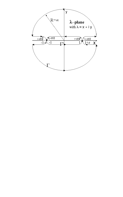
Figure 1: Contours $\Gamma^{\prime}$ (smaller one) and $\Gamma$ (larger one). Bold lines $(-\infty,-1-\epsilon)$ and $(1+\epsilon,\infty)$ are the cuts of the integrand $e(1+\epsilon,\lambda)$. Zeros of $D_{L}(\lambda)$ (Eq. 16) are located on the bold line $(-1,1)$. The arrows indicate the directions of integrations, and $\mathrm{r}$ and $\mathrm{R}$ are the radius of the circles. $\P$

We also notice that $\widetilde{\mathbf{B}}_{L}(\lambda)$ is the block Toeplitz matrix,

$$\widetilde{\mathbf{B}}_{L}(\lambda)=\left(\begin{array}[]{cccc}\widetilde{\Pi}_{0}&\widetilde{\Pi}_{-1}&\ldots&\widetilde{\Pi}_{1-L}\\ \widetilde{\Pi}_{1}&\widetilde{\Pi}_{0}&&\vdots\\ \vdots&&\ddots&\vdots\\ \widetilde{\Pi}_{L-1}&\ldots&\ldots&\widetilde{\Pi}_{0}\end{array}\right)\quad\textrm{with}$$ (22)

$$\widetilde{\Pi}_{l}=\frac{1}{2\pi\mathrm{i}}\oint_{\Xi}\,\mathrm{d}z\,z^{-l-1}\Phi(z),$$ (23)

where the matrix generator $\Phi(z)$ is defined by the equations,

$$\Phi(z)=\left(\begin{array}[]{cc}\mathrm{i}\lambda&\phi(z)\\ -\phi^{-1}(z)&\mathrm{i}\lambda\end{array}\right)$$ (24)

$$\textrm{and}\quad\phi(z)=\left(\frac{\lambda_{1}^{*}}{\lambda_{1}}\frac{(1-\lambda_{1}\,z)(1-\lambda_{2}\,z^{-1})}{(1-\lambda_{1}^{*}\,z^{-1})(1-\lambda_{2}^{*}\,z)}\right)^{1/2}$$ (25)

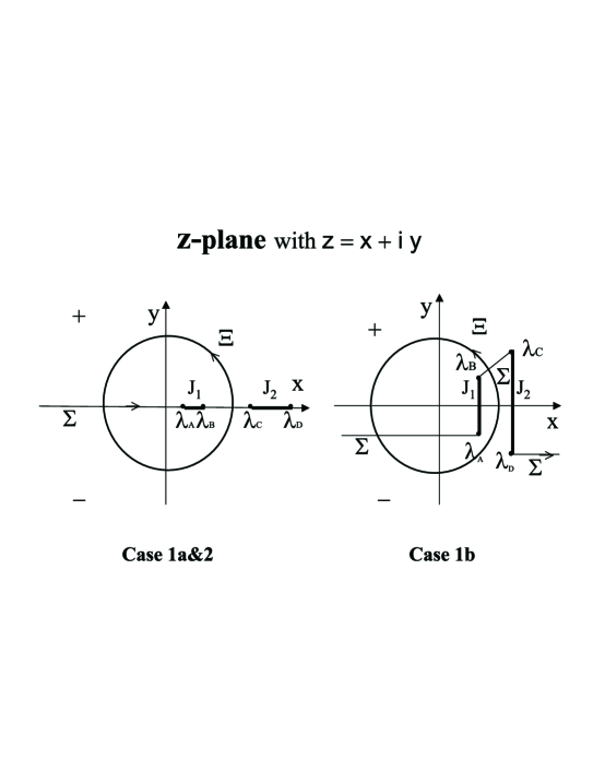
Figure 2: The polygonal line $\Sigma$ (oriented as it is indicated) separates the complex $z$ plane into two parts: the part $\Omega_{+}$ which lies to the left of $\Sigma$, and the part $\Omega_{-}$ which lies to the right of $\Sigma$. Curve $\Xi$ is the unit circle in anti-clockwise direction. Cuts $J_{1},J_{2}$ for the functions $\phi(z),w(z)$ are labeled by bold on the line $\Sigma$. The definition of the end points of the cuts $\lambda_{\ldots}$ depends on the case: Case $1$a: $\lambda_{A}=\lambda_{1}$, $\lambda_{B}=\lambda_{2}^{-1}$, $\lambda_{C}=\lambda_{2}$, and $\lambda_{D}=\lambda_{1}^{-1}$. Case $1$b: $\lambda_{A}=\lambda_{1}$, $\lambda_{B}=\lambda_{2}^{-1}$, $\lambda_{C}=\lambda_{1}^{-1}$, and $\lambda_{D}=\lambda_{2}$. Case $2$: $\lambda_{A}=\lambda_{1}$, $\lambda_{B}=\lambda_{2}$, $\lambda_{C}=\lambda_{2}^{-1}$, and $\lambda_{D}=\lambda_{1}^{-1}$. $\P$

We fix the branch of $\phi(z)$ by requiring that $\phi(\infty)>0$. We use $*$ to denote complex conjugation, and $\Xi$ is the unit circle shown in Fig. 2. The points $\lambda_{1}$ and $\lambda_{2}$ are defined differently for the different values of $\gamma$ and $h$.

There are three different cases:

Case $1$a is defined by inequality $4{(1-\gamma^{2})}<h^{2}<4$ .

It describes moderate magnetic field.

Case $2$ is defined by $h>2$. This is strong magnetic field.

In both cases $\lambda_{1}$ and $\lambda_{2}$ are real and given by the formulae

$$\lambda_{1}=\frac{h-\sqrt{h^{2}-4(1-\gamma^{2})}}{2(1+\gamma)},\quad\lambda_{2}=\frac{1+\gamma}{1-\gamma}\lambda_{1}.$$ (26)

Case $1$b is defined by $h^{2}<4(1-\gamma^{2})$.

It is weak magnetic field, including zero magnetic field.

Both $\lambda_{1}$ and $\lambda_{2}$ are complex and given by the equations

$$\lambda_{1}=\frac{h-\mathrm{i}\sqrt{4(1-\gamma^{2})-h^{2}}}{2(1+\gamma)},\quad\lambda_{2}=1/\lambda_{1}^{*}.$$ (27)

Note that in Case $1$ the poles of the function $\phi(z)$ (Eq. 25) coincide with the points $\lambda_{A}$ and $\lambda_{B}$, while in Case $2$ they coincide with the points $\lambda_{A}$ and $\lambda_{C}$.

We are going now to formulate our main results. To this end we need to introduce the Jacobi theta-function,

$$\theta_{3}(s)=\sum_{n=-\infty}^{\infty}e^{\pi i\tau n^{2}+2\pi isn}.$$ (28)

We remind the following characteristic properties of this function (see e.g. [39]):

$$\theta_{3}(-s)=\theta_{3}(s),\quad\theta_{3}(s+1)=\theta_{3}(s)$$ (29)

$$\theta_{3}(s+\tau)=e^{-\pi i\tau-2\pi is}\theta_{3}(s)$$ (30)

$$\theta_{3}\left(n+m\tau+\frac{1}{2}+\frac{\tau}{2}\right)=0,\quad n,m\in{\mbox{\mybbb Z}}$$ (31)

The modulus parameter $\tau$, in our case, is determined by the physical quantities $h$ and $\gamma$ according to the following equation

$$\tau=i\tau_{0},\quad\tau_{0}=I(k^{\prime})/I(k)$$ (32)

where $I(k)$ denotes the complete elliptic integral of the first kind,

$$I(k)=\int_{0}^{1}\frac{dx}{\sqrt{(1-x^{2})(1-k^{2}x^{2})}}\qquad\qquad\diamond$$

also $k^{\prime}=\sqrt{1-k^{2}}$, and

$$k=\left\{\begin{array}[]{c}\sqrt{(h/2)^{2}+\gamma^{2}-1}\;/\;\gamma,\;\;\;\mbox{Case 1a}\\[8.5359pt] \sqrt{1-\gamma^{2}-(h/2)^{2}}\;/\;\sqrt{1-(h/2)^{2}},\;\;\;\mbox{Case 1b}\\[8.5359pt] \gamma\;/\;\sqrt{(h/2)^{2}+\gamma^{2}-1},\;\;\;\mbox{Case 2}\end{array}\right.$$ (36)

Define also the function

$$\beta(\lambda)=\frac{1}{2\pi i}\ln\frac{\lambda+1}{\lambda-1},$$ (37)

and the infinite sequence of real numbers,

$$\lambda_{m}=\tanh\left(m+\frac{1-\sigma}{2}\right)\pi\tau_{0},\quad m\geq 0,$$ (38)

where $\sigma=1$ in Case 1 and $\sigma=0$ in Case 2. Observe that

• $0<\lambda_{m}<1,\quad\lambda_{m}\to 1,\quad m\to\infty$

• in view of Eq. (31), the points $\pm\lambda_{m}$ are zeros of $\theta_{3}\left(\beta(\lambda)+\frac{\sigma\tau}{2}\right)$.

Theorem 1. Let $\Omega$ be the complex $\lambda$ - plane without arbitrary fixed neighborhoods of the points $\lambda=\infty$, $\lambda=\pm 1$ and $\lambda=\pm\lambda_{m},\quad m=0,1,...$ . Then the Toeplitz determinant $D_{L}(\lambda)$ admits the following asymptotic representation, which is uniform in $\lambda\in\Omega$.

$$\frac{d}{d\lambda}\ln D_{L}(\lambda)=-\frac{2\lambda}{1-\lambda^{2}}L+\frac{d}{d\lambda}\ln\left[\theta_{3}\left(\beta(\lambda)+\frac{\sigma\tau}{2}\right)\theta_{3}\left(\beta(\lambda)-\frac{\sigma\tau}{2}\right)\right]$$ (39)

$$+O\left(\rho^{-L}\right),\quad L\to\infty.$$

Here $\rho$ is any positive number satisfying the inequality,

$$1<\rho<|\lambda_{C}|.$$

This theorem shows that in the large $L$ limit, the points $\pm\lambda_{m}$ (38) are double zeros of the $D_{L}(\lambda)$. More precisely, we see that in the large $L$ limit the eigenvalues $\nu_{2m}$ and $\nu_{2m+1}$ from (12), (11) merge to $\lambda_{m}$:

$$\nu_{2m},\nu_{2m+1}\to\lambda_{m},$$ (40)

which in turn implies our main result:

The limiting entropy, $S(\rho_{A})$, of the subsystem can be identified with the infinite convergent series,

$$\diamondsuit\quad\qquad S(\rho_{A})=\sum_{m=-\infty}^{\infty}H(\lambda_{m})=\sum_{m=-\infty}^{\infty}(1+\lambda_{m})\ln\frac{2}{1+\lambda_{m}}\qquad\diamondsuit$$ (41)

It is worth mentioning that relation (40) also indicates the degeneracy of the spectrum of the matrix ${\bf B}_{L}$ and an appearance of an extra symmetry in the large $L$ limit.

Observe that equation (17) can be also rewritten as

$$S_{L}(\rho_{A})=\lim_{\epsilon\to 0^{+}}\frac{1}{4\pi\mathrm{i}}\oint_{\Gamma^{\prime}}\mathrm{d}\lambda\,e(1+\epsilon,\lambda)\frac{\mathrm{d}}{\mathrm{d}\lambda}\ln\left(D_{L}(\lambda)(\lambda^{2}-1)^{-L}\right)\;,$$ (42)

because of the following identity

$$\lim_{\epsilon\to 0^{+}}\oint_{\Gamma^{\prime}}\mathrm{d}\lambda\,e(1+\epsilon,\lambda)\frac{\mathrm{d}}{\mathrm{d}\lambda}\ln(\lambda^{2}-1)^{-L}=L\lim_{\epsilon\to 0^{+}}\oint_{\Gamma^{\prime}}\mathrm{d}\lambda\,e(1+\epsilon,\lambda)\frac{2\lambda}{1-\lambda^{2}}$$

$$=2\pi iL\lim_{\epsilon\to 0^{+}}\left((2+\epsilon)\ln{\frac{2+\epsilon}{2}}+\epsilon\ln{\frac{\epsilon}{2}}\right)=0.$$

In this paper, we will show that series (41) coincides with the result of the following double limit procedure

$$S(\rho_{A})=\lim_{\epsilon\to 0^{+}}\left[\lim_{L\to\infty}\frac{1}{4\pi\mathrm{i}}\oint_{\Gamma^{\prime}}\mathrm{d}\lambda\,e(1+\epsilon,\lambda)\frac{\mathrm{d}}{\mathrm{d}\lambda}\ln\left(D_{L}(\lambda)(\lambda^{2}-1)^{-L}\right)\right]\;,$$ (43)

here the contour $\Gamma^{\prime}$ is depicted in Fig 1. This result can be alternatively written down as the following integral,

$$\clubsuit\qquad S(\rho_{A})=\frac{1}{2}\int_{1}^{\infty}\ln\left(\frac{\theta_{3}\left(\beta(\lambda)+\frac{\sigma\tau}{2}\right)\theta_{3}\left(\beta(\lambda)-\frac{\sigma\tau}{2}\right)}{\theta^{2}_{3}\left(\frac{\sigma\tau}{2}\right)}\right)\,d\lambda.\quad\spadesuit$$ (44)

We conjecture that in fact the limits in (43) can be interchanged. After the shorten version of this paper appeared in quant-ph, I.Peschel [67] simplified our expression for the entropy for non-vanishing magnetic field [Cases 1a and 2]. He used the approach of [12]. He showed that in these cases our formula (41) is equivalent to formula (4.33) of [12]. Moreover, I. Peschel was able to sum it up into the following expressions for the entropy.

$$S(\rho_{A})=\frac{1}{6}\left[\;\ln{\left(\frac{k^{2}}{16k^{\prime}}\right)}+\left(1-\frac{k^{2}}{2}\right)\frac{4I(k)I(k^{\prime})}{\pi}\right]+\ln\;2,$$ (45)

in Case 1a, and

$$S(\rho_{A})=\frac{1}{12}\left[\;\ln{\frac{16}{(k^{2}k^{\prime 2})}}+(k^{2}-k^{\prime 2})\frac{4I(k)I(k^{\prime})}{\pi}\right],$$ (46)

in Case 2 . Here, $I(k)$ denotes the complete elliptic integral of the first kind, $k^{\prime}=\sqrt{1-k^{2}}$, and

$$k=\left\{\begin{array}[]{c}\sqrt{(h/2)^{2}+\gamma^{2}-1}\;/\;\gamma,\;\;\;\mbox{Case 1a}\\[8.5359pt] \gamma\;/\;\sqrt{(h/2)^{2}+\gamma^{2}-1},\;\;\;\mbox{Case 2}\end{array}\right.$$ (49)

These describes cases of moderate and strong magnetic field.

We used the equation (41) to calculate limiting entropy for weak magnetic field.

In Case 1b we derived:

$$S(\rho_{A}) =\frac{1}{6}\left[\;\ln{\left(\frac{k^{2}}{16k^{\prime}}\right)}+\left(1-\frac{k^{2}}{2}\right)\frac{4I(k)I(k^{\prime})}{\pi}\right]+\ln\;2,$$

$$k=\sqrt{\frac{1-h^{2}/4-\gamma^{2}}{1-h^{2}/4}}\qquad\qquad\qquad\heartsuit$$

iff $$0\leq h<2\sqrt{1-\gamma^{2}}$$ (50)

Note that this case includes zero magnetic field.

These expressions helped us to study the range of variation of limting entropy. Together with Dr. Franchini we found that the entropy has a local minimum at the boundary of Cases 1a and 1b:

$$S(\rho)=\ln 2\qquad\mbox{at}\qquad\left(\frac{h}{2}\right)^{2}+\gamma^{2}=1\qquad\qquad\star$$

At this boundary the ground state is doubly degenerated, but the rest of energy levels are separated by a gap.

Note that the absolute minimum of asymptotic entropy $\min S(\rho)=0$ is achieved at infinite magnetic field corresponding to $k=0$ in Case 2 [the ground state is ferromagnetic]

2 The Asymptotic of Block Toeplitz Determinants, Widom’s Theorems.

Our objective is the asymptotic calculation of the block Toeplitz determinant $D_{L}(\lambda)$ or, rather, its $\lambda$ -derivative $\frac{d}{d\lambda}\ln D_{L}(\lambda)$. A general asymptotic representation of the determinant of a block Toeplitz matrix, which generalizes the classical strong Szegö theorem to the block matrix case, was obtained by H. Widom in [55] (see also more recent work [64] and references therein). Here is Widom’s result.

Let

$$\varphi(z)=\sum_{k=-\infty}^{\infty}\varphi_{k}z^{k},\quad|z|=1,$$

be an $p\times p$ matrix - valued function defined on the unite circle, $|z|=1$, and satisfying the following conditions.

1. $||\varphi||\equiv\sum_{k=-\infty}^{\infty}||\varphi_{k}||+\left\{\sum_{k=-\infty}^{\infty}|k|||\varphi_{k}||^{2}\right\}^{1/2}<\infty$

2. $\det\varphi(z)\neq 0,\quad\Delta|_{|z|=1}\arg\det\varphi(z)=0$

Consider the block Toeplitz determinant generated by $\varphi(z)$, i.e. $D_{L}[\varphi]=\det T_{L}[\varphi]$ where $T_{L}[\varphi]=\left(\varphi_{j-k}\right)$, $j,k=0,...,L-1$.

Theorem 2. ([56])Define

$$G[\varphi]=\exp\left\{\frac{1}{2\pi i}\int_{|z|=1}\ln\det\varphi(z)\frac{dz}{z}\right\}.$$ (51)

Then the limit

$$E[\varphi]={\lim_{L\to\infty}\frac{D_{L}[\varphi]}{\left(G[\varphi]\right)^{L}}}\,\,,$$ (52)

exists. Moreover, the following general formula can be written for the quantity $E[\varphi]$,

$$E[\varphi]=\det\left(T_{\infty}[\varphi]T_{\infty}[\varphi^{-1}]\right).$$ (53)

This quite beautiful theorem is not very efficient in concrete applications. The remarkable fact though is that the proof of theorem 2 is based on an auxiliary fact which was established in the preceding work of Widom and which can be made an efficient tool for a large class of symbols $\varphi$, including the matrix function $\Phi(z)$ from (24) which we are concerned with in this paper.

Theorem 3 (theorem 4.1 of [55])Suppose that, in addition to the conditions of theorem 2, the matrix symbol $\varphi^{-1}$ admits the Weiner-Hopf factorization,

$$\varphi^{-1}(z)=u_{+}(z)u_{-}(z)=v_{-}(z)v_{+}(z),$$ (54)

where the subscribes “+” and “-” indicate the analyticity inside and outside of the unite circle, respectively. Suppose also that $\varphi(z)$ can be included into a differentiable family, $\lambda\to\varphi(z,\lambda)$. Then, $\ln E[\varphi]$ is a differentiable function of $\lambda$ and in fact,

$$\frac{d}{d\lambda}\ln E[\varphi]=\frac{i}{2\pi}\int_{|z|=1}trace\left[\left(u^{\prime}_{+}(z)u_{-}(z)-v^{\prime}_{-}(z)v_{+}(z)\right)\frac{\partial\varphi(z,\lambda)}{\partial\lambda}\right]dz,$$ (55)

where $(^{\prime})$ means the derivative with respect to $z$.

Let $\Omega$ be the set on the $\lambda$ - plane introduced in theorem 1. In the next section we will show that for every $\lambda\in\Omega$, the matrix-valued function $\Phi(z)$ admits the explicit Weiner-Hopf factorization, and hence the second Widom theorem - theorem 3 above, is applicable. Indeed, for the function $\Phi(z)$ this theorem can be specified as follows.

Theorem 4. Let $\lambda\in\Omega$ then the following asymptotic representation for the logarithmic derivative of the determinant $D_{L}(\lambda)=\det T_{L}[\Phi]$ takes place.

$$\frac{d}{d\lambda}\ln D_{L}(\lambda)=-\frac{2\lambda}{1-\lambda^{2}}L\$$

$$+\frac{1}{2\pi}\int_{|z|=1}\mbox{trace}\,\Bigl{[}\left(U_{+}^{\prime}(z)U_{+}^{-1}(z)+V_{+}^{-1}(z)V_{+}^{\prime}(z)\right)\Phi^{-1}(z)\Bigr{]}dz$$ (56)

$$+r_{L}(\lambda),$$

where the error term $r_{L}(\lambda)$ satisfies the uniform estimate,

$$|r_{L}(\lambda)|\leq C\rho^{-L},\quad\quad\lambda\in\Omega,\quad L\geq 1,$$ (57)

and $\rho$ is any positive number such that $1<\rho<|\lambda_{C}|$. In (56) the $2\times 2$ matrix-valued functions $U_{\pm}(z)$ and $V_{\pm}(z)$ solve the following Weiner-Hopf factorization problem :

(i) $\Phi(z)=U_{+}(z)U_{-}(z)=V_{-}(z)V_{+}(z)\quad z\in\Xi$

(ii)  $U_{-}(z)$ and $V_{-}(z)$ ($U_{+}(z)$ and $V_{+}(z)$) are analytic outside (inside) the unit circle $\Xi$.

(iii)  $U_{-}(\infty)=V_{-}(\infty)=I$.

Remark . The replacement of the factorization of the inverse symbol by the factorization of the symbol itself has been made for a purely technical reason.

Asymptotic representation (56) plays an important role in our analysis as, in fact, its starting point. The truth of the matter is that we had derived formula (56) before we became aware of Widom’s second theorem. In our original derivation of (56) and proof of theorem 4 we used an alternative approach to Toeplitz determinants suggested by P. Deift in [31]. It is based on the Riemann-Hilbert technique of the theory of “integrable integral operators”, which was developed in [33], [66] for evaluation of correlation functions of quantum completely integrable (exactly solvable) models . It turns out that, using the block matrix version of [33] suggested in [37], one can generalize Deift’s scheme to the block Toeplitz matrices, which provides a rather simple derivation of equation (56) together with the estimation of the error term indicated in theorem 4.

The Riemann-Hilbert approach has already proved its usefulness in the theory of Toeplitz and Hankel determinants with scalar symbols (see e.g. [57], [72], [58], [59], [60]). Therefore, we believe that the block-version of the Riemann-Hilbert scheme is worthwhile to present. Indeed, although in the relatively simple case of smooth symbols theorem 4, as it turned out, is a direct (up to the error term estimation) corollary of one of the old Widom’s results, it is conceivable that in more challenging situations of the matrix symbols with singularities the Riemann-Hilbert scheme might become very useful, as it has been already the case for the scalar symbols.

Having all the above reasons in mind, we have decided to include in the paper our original proof of theorem 4. We will do this in the next section providing all the necessary facts concerning integrable Fredholm operators and the Riemann-Hilbert method of their analysis.

The explicit factorization of the matrix $\Phi(z)$ will be performed in section 4 and the final proof of our main result - theorem 1, will be done in section 5.

3 The Riemann-Hilbert approach to the block Toeplitz determinants. An alternative proof of theorem 4.

3.1 The Fredholm Determinant Representation

Let $f_{j}(z)$ and $h_{j}(z)$, $j=1,2$, be $2\times 2$ matrix functions. We introduce the class of integrable operators $K$ defined on $L_{2}(\Xi,{\mbox{\mybbb C}}^{2})$ by the following equations (cf. [37]),

$$(K\,X)(z)=\oint_{\Xi}K(z,z^{\prime})\,X(z^{\prime})dz^{\prime}\quad\textrm{for}\quad X\in L_{2},$$ (58)

where

$$K(z,z^{\prime})=\frac{f^{T}(z)h(z^{\prime})}{z-z^{\prime}},\quad f(z)=\left(\begin{array}[]{c}f_{1}^{T}(z)\\ f_{2}^{T}(z)\end{array}\right)$$

$$h(z)=\left(\begin{array}[]{c}h_{1}(z)\\ h_{2}(z)\end{array}\right).$$ (59)

Let $I_{2}$ denote the $2\times 2$ identity matrix. Put

$$f_{1}(z)=z^{L}I_{2},\quad f_{2}(z)=I_{2}$$ (60)

$$h_{1}(z)=z^{-L}\frac{I_{2}-\Phi(z)}{2\pi i},\quad h_{2}(z)=-\frac{I_{2}-\Phi(z)}{2\pi i}.$$ (61)

Then, essentially repeating the arguments of [31], we have the following relation

$$D_{L}(\lambda)=\det(I-K),$$ (62)

where $I$ is the identity operator in $L_{2}(\Xi,{\mbox{\mybbb C}}^{2})$. The determinant in the l.h.s. is the $2L\times 2L$ matrix determinant, while the (Fredholm) determinant in the r.h.s. is taken in $L_{2}(\Xi,{\mbox{\mybbb C}}^{2})$. This relation can be proved by writing down the matrix representation of the integral operator $I-K$ in the basis $\{z^{k}e_{j}\}_{-\infty<k<\infty,\,j=1,2}$, where $\{e_{1},e_{2}\}$ is the canonical basic in ${\mbox{\mybbb C}}^{2}$ (cf. [31]). The matrix elements of operator $I-K$ can be defined by following relations:

$$(I-K)z^{k}\,e_{\alpha}=\sum_{j=0}^{L-1}\sum_{\beta=1}^{2}\Phi_{\beta,\alpha}^{j-k}z^{j}\,e_{\beta},\quad\qquad\qquad 0\leq k<L,\quad\alpha=\{1,2\},$$ (63)

$$(I-K)z^{k}\,e_{\alpha}=z^{k}\,e_{\alpha}+\sum_{j=0}^{L-1}\sum_{\beta=1}^{2}\Phi_{\beta,\alpha}^{j-k}z^{j}\,e_{\beta},\quad k<0~{}\textrm{or}~{}k\geq L,\quad\alpha=\{1,2\}.$$ (64)

Here

$$\Phi_{\beta,\alpha}^{j}=\frac{1}{2\pi i}\int_{|z|=1}\Bigl{(}\Phi(z)\Bigr{)}_{\beta,\alpha}\frac{dz}{z^{j+1}}\equiv(\widetilde{\Pi}_{j})_{\beta,\alpha}.$$

With $\widetilde{\mathbf{B}}_{L}(\lambda)$ defined as $(\Phi_{\beta,\alpha}^{j-k})$, $0\leq j,k\leq L-1$; $\alpha,\beta$ taking $1$ or $2$; $(j,\beta)$ numerating the rows and $(k,\alpha)$ numerating the columns , equation (62) becomes obvious.

So we represented $D_{L}(\lambda)$ as a Fredholm determinant of the integral operator $K$. Define the resolvent operator $R$ by

$$(I-K)(I+R)=I\quad\Leftrightarrow\quad R=(I-K)^{-1}K.$$

Then, we have the general equation [33], [37],

$$R(z,z^{\prime})=\frac{F^{T}(z)H(z^{\prime})}{z-z^{\prime}},$$ (65)

where

$$F^{T}=(I-K)^{-1}f^{T},\quad\mbox{and}\quad H=h(I-K)^{-1}$$

where in the first equation $(I-K)^{-1}$ is understood as acting to the right, while in the second equation it acts to the left.

3.2 The Riemann-Hilbert Problem

One of the main ingredients of the theory of integrable operators is the following Riemann-Hilbert representation for the functions $F(z)$ and $H(z)$.

$$F(z)=Y_{+}(z)f(z),\quad z\in\Xi,$$ (66)

$$H(z)=(Y^{T}_{+})^{-1}(z)h(z),\quad z\in\Xi,$$ (67)

where the $4\times 4$ matrix function $Y(z)$ is the (unique) solution of the following Riemann-Hilbert problem:

1. $Y(z)$ is analytic outside of the circle $\Xi$.

2. $Y(\infty)=I_{4}$, where $I_{4}$ denote the $4\times 4$ identity matrix.

3. $Y_{-}(z)=Y_{+}(z)J(z),\quad z\in\Xi$ where $Y_{+}(z)$ ($Y_{-}(z)$) denote the left (right) boundary value of $Y(z)$ on $\Xi$ (note, “+” means: from inside of the unite circle!). The $4\times 4$ jump matrix $J(z)$ is defined by the equations,

   $$J(z)=I_{4}+2\pi if(z)h^{T}(z)$$

   $$=\left(\begin{array}[]{cc}2I_{2}-\Phi^{T}(z)&-z^{L}(I_{2}-\Phi^{T}(z))\\ z^{-L}(I_{2}-\Phi^{T}(z))&\Phi^{T}(z)\end{array}\right)$$ (68)

It is also worth noticing the integral formulae,

$$Y(z)=I_{4}-\int_{\Xi}\frac{F(z^{\prime})h^{T}(z^{\prime})}{z^{\prime}-z}dz^{\prime},$$ (69)

and

$$Y^{-1}(z)=I_{4}+\int_{\Xi}\frac{f(z^{\prime})H^{T}(z^{\prime})}{z^{\prime}-z}dz^{\prime}.$$ (70)

We are going now to relate the $\lambda$ - derivative of $\det(I-K)$ and the resolvent. To this end we first notice that

$$\frac{d}{d\lambda}\Phi(z)=iI_{2}.$$

Therefore, we have that,

$$\frac{d}{d\lambda}K(z,z^{\prime})=-\frac{1}{2\pi}\frac{z^{L}(z^{\prime})^{-L}-1}{z-z^{\prime}}\,I_{2}\equiv-iK(z,z^{\prime})(I_{2}-\Phi(z^{\prime}))^{-1}.$$

From this it follows that

$$\left[(I-K)^{-1}\frac{d}{d\lambda}K\right](z,z^{\prime})=-iR(z,z^{\prime})(I_{2}-\Phi(z^{\prime}))^{-1},$$

and hence

$$\frac{d}{d\lambda}\ln\det T_{L}\{\phi\}=-\mbox{Trace}\,(I-K)^{-1}\frac{d}{d\lambda}K$$

$$=i\int_{\Xi}\mbox{trace}\,\left(R(z,z)(I_{2}-\Phi(z))^{-1}\right)dz,$$ (71)

where “Trace” means the trace taking in the space $L_{2}(\Xi,{\mbox{\mybbb C}}^{2})$, while “trace” is the $2\times 2$ matrix trace.

From (65) we conclude that

$$R(z,z)=\frac{dF^{T}(z)}{dz}H(z),$$

which in turn implies the equation

$$\frac{d}{d\lambda}\ln\det T_{L}\{\phi\}=i\int_{\Xi}\mbox{trace}\,\left(\frac{dF^{T}(z)}{dz}H(z)(I_{2}-\Phi(z))^{-1}\right)dz.$$ (72)

3.3 The Asymptotic Solution of the Riemann-Hilbert Problem.

Equation (72), together with (66) and (67) it reduces the question to the asymptotic analysis of the solution $Y(z)$ of the Riemann-Hilbert problem (1 - 3). For the latter we shall follow [31].

The basic observation is that the jump matrix $J(z)$ admits the following algebraic factorization,

$$J(z)=M(z)J_{0}(z)N(z),$$ (73)

. where

$$M(z)=\left(\begin{array}[]{cc}I_{2}&z^{L}\left(I_{2}-(\Phi^{T})^{-1}(z)\right)\\ 0_{2}&I_{2}\end{array}\right),$$ (74)

$$N(z)=\left(\begin{array}[]{cc}I_{2}&0_{2}\\ -z^{-L}\left(I_{2}-(\Phi^{T})^{-1}(z)\right)&I_{2}\end{array}\right),$$ (75)

and

$$J_{0}(z)=\left(\begin{array}[]{cc}(\Phi^{T})^{-1}(z)&0_{2}\\ 0_{2}&\Phi^{T}(z)\end{array}\right).$$ (76)

Choose now a small $\epsilon$ and define the matrix function $X(z)$ according to the equations:

$$X(z)=Y(z)\quad\mbox{if}\quad|z|>1+\epsilon,\quad\mbox{or}\quad|z|<1-\epsilon,$$ (77)

$$X(z)=Y(z)M(z)\quad\mbox{if}\quad 1-\epsilon<|z|<1,$$ (78)

$$X(z)=Y(z)N^{-1}(z)\quad\mbox{if}\quad 1<|z|<1+\epsilon.$$ (79)

The new function has a jump accross the unit circle $\Xi$ with the jump matrix $J_{0}(z)$ and two more jumps - accross the circles,

$$\Xi_{1}:|z|=1-\epsilon,\quad\mbox{jump matrix}\,\,M(z)$$

and

$$\Xi_{2}:|z|=1+\epsilon,\quad\mbox{jump matrix}\,\,N(z).$$

In other words, the original Rimeann-Hilbert problem (1 - 3) is equivalent to the problem

1⁰. $X(z)$ is analytic outside of the contour $\Gamma\equiv\Xi\cup\Xi_{1}\cup\Xi_{2}$.

2⁰. $X(\infty)=I_{4}$, where $I_{4}$ denote the $4\times 4$ identity matrix.

3⁰. The jumps of the function $X(z)$ across the contour $\Gamma$ are given by the equations

• $X_{-}(z)=X_{+}(z)M(z),\quad z\in\Xi_{1}$

• $X_{-}(z)=X_{+}(z)N(z),\quad z\in\Xi_{2}$

• $X_{-}(z)=X_{+}(z)J_{0}(z),\quad z\in\Xi$

where the jump matrices $M(z)$, $N(z)$, and $J_{0}(z)$ are defined in (74), (75), and (76), respectively and each circle is oriented counterclockwise.

Observe that the differences of the jump matrices on $\Xi_{1}$ and $\Xi_{2}$ from the identity are exponentially small as $n\to\infty$. This means one can expect the following asymptotic relation for $X(z)$,

$$X(z)\sim X^{0}(z),$$ (80)

where the independent on $L$ function $X^{0}(z)$ solves the Riemann-Hilbert problem which is the same as the $Y$ - problem but with the jump matrix $J_{0}(z)$ instead of $J(z)$.

We notice that the function $X^{0}(z)$ can be found explicitly in terms of the $2\times 2$ matrix-valued functions $U_{\pm}(z)$ and $V_{\pm}(z)$ solving the following Weiner-Hopf factorization problem :

(i) $\Phi(z)=U_{+}(z)U_{-}(z)=V_{-}(z)V_{+}(z),\quad z\in\Xi$

(ii)  $U_{-}(z)$ and $V_{-}(z)$ ($U_{+}(z)$ and $V_{+}(z)$) are analytic outside (inside) the unit circle $\Xi$.

(iii)  $U_{-}(\infty)=V_{-}(\infty)=I$.

Indeed we have that

$$X^{0}(z)=\left(\begin{array}[]{cc}U_{+}^{T}(z)&0_{2}\\ 0_{2}&(V_{+}^{T})^{-1}(z)\end{array}\right),\quad\mbox{if}\quad|z|<1,$$ (81)

and

$$X^{0}(z)=\left(\begin{array}[]{cc}(U_{-}^{T})^{-1}(z)&0_{2}\\ 0_{2}&V_{-}^{T}(z)\end{array}\right),\quad\mbox{if}\quad|z|>1.$$ (82)

In the next section, we will show that for all $\lambda\in\Omega$ the above Weiner-Hopf factorization can be found explicitely, in terms of the elliptic theta-functions. In this section though we won’t need the explicit formulae for $U_{\pm}(z)$ and $V_{\pm}(z)$. The only information we will need in this section is the existence of $U_{\pm}(z)$ and $V_{\pm}(z)$, and the uniform estimate

$$|U_{\pm}(z)|,\quad|V_{\pm}(z)|<C,\quad\forall z,\quad\forall\lambda\in\Omega,$$ (83)

which is the direct consequence of the explicit formulae (154), (155), and (107), (108) of section 4.

We are now ready to formulate and prove the rigorous version of the formal asymptotic relation (80).

Theorem 5. Let $\Omega$ be the set introduced in theorem 1, i.e. the complex $\lambda$-plane without arbitrary fixed neighborhoods of the points $\lambda=\infty$, $\lambda=\pm 1$, and $\lambda=\pm\lambda_{m}$, $m=0,1,...$, where $\lambda_{m}$ are defined in (156) . Then, for sufficiently large $L$ and all $\lambda\in\Omega$, the Riemann-Hilbert problem (1⁰ - 3⁰) has the unique solution $X(z)$ which satisfies the following uniform estimate,

$$\left|X(z)\left(X^{0}(z)\right)^{-1}-I_{4}\right|\leq C\frac{\rho^{-L}}{1+|z|},\quad z\in{\mbox{\mybbb C}},\quad\lambda\in\Omega,\quad L\geq L_{0},$$ (84)

where $\rho$ is any positive number such that $1<\rho<|\lambda_{C}|$, and the block diagonal matrix-valued function $X^{0}(z)$ is defined by the equations (81) and (82).

Proof. Put

$$R(z):=X(z)\left(X^{0}(z)\right)^{-1}.$$

Observe that since $\det J_{0}(z)\equiv 1$, the function $d(z)=\det X^{0}(z)$ solves the following scalar Riemann-Hilbert problem:

• $d(z)$ is analytic outside the unit circle $\Xi$

• $d_{-}(z)=d_{+}(z)$, $z\in\Xi$

• $d(\infty)=1$

By virtue of the Liouville theorem, this implies that $d(z)=\det X^{0}(z)\equiv 1$, and hence the matrix ratio $R(z)$ is well defined. In fact, in terms of the matrix function $R(z)$ the Riemann-Hilbert problem (1⁰ - 3⁰) can be rewritten as follows .

1⁰⁰. $R(z)$ is analytic outside of the contour $\Gamma_{0}\equiv\Xi_{1}\cup\Xi_{2}$ (no jump across the unite circle $\Xi$!).

2⁰⁰. $R(\infty)=I_{4}$, where $I_{4}$ denote the $4\times 4$ identity matrix.

3⁰⁰. The jumps of the function $R(z)$ across the contour $\Gamma_{0}$ are given by the equations

• $R_{-}(z)=R_{+}(z)\hat{M}(z),\quad z\in\Xi_{1}$

• $R_{-}(z)=R_{+}(z)\hat{N}(z),\quad z\in\Xi_{2}$

where the jump matrices $\hat{M}(z)$ and $\hat{N}(z)$ are defined by the formulae

$$\hat{M}(z)=X^{0}(z)M(z)[X^{0}(z)]^{-1},\quad\hat{N}(z)=X^{0}(z)N(z)[X^{0}(z)]^{-1}.$$ (85)

Let us denote $G_{0}(z)$ the jump matrix of the function $R(z)$, i.e.

$$G_{0}(z)=\left\{\begin{array}[]{c}\hat{M}(z),\quad z\in\Xi_{1}\\[8.5359pt] \hat{N}(z),\quad z\in\Xi_{2}\end{array}\right.$$ (88)

Then, taking into account the estimate (83) and the expressions for matrices $M(z)$ and $N(z)$ we immediately arrive at the estimate,

$$|I_{4}-G_{0}(z)|\leq C\rho^{-L},\quad 1<\rho<|\lambda_{C}|,\quad z\in\Gamma_{0},\quad\lambda\in\Omega,\quad L\geq 1.$$ (89)

This in turn implies the $L_{2}\cap L_{\infty}$ - norm estimate:

$$\|I_{4}-G_{0}\|_{L_{2}(\Gamma_{0})\cap L_{\infty}(\Gamma_{0})}\leq C\rho^{-L},$$ (90)

which, by standard arguments based on the analysis of the relevant singular integral equation (see e.g. [58] or Appendix D of [72]), yields the estimate (84). For the reader’s convenience we will now present those arguments.

According to the general theory of Riemann-Hilbert problems (see e.g. [61] or [62]) the solution $R(z)$ of the Riemann-Hilbert problem (1⁰⁰ - 3⁰⁰) is given by the integral representation,

$$R(z)=I+{1\over 2\pi i}\int_{\Gamma_{0}}r(z^{\prime})\left(I_{4}-G_{0}(z^{\prime})\right){dz^{\prime}\over{z^{\prime}-z}},\quad z\not\in\Gamma_{0},$$ (91)

where $r(z)\equiv R_{+}(z)$ solves the singular integral equation

$$r(z)=I+C_{+}[r\left(I_{4}-G_{0}\right)](z),\quad z\in\Gamma_{0},$$ (92)

and $C_{+}$ is the corresponding Cauchy operator:

$$(C_{+}h)(z)=\lim_{z^{\prime}\to z,\,z^{\prime}\in(+)-\mbox{side}}\int_{\Gamma_{0}}{h(s)\over{s-z^{\prime}}}\,{ds\over 2\pi i}.$$

We note that in the case under consideration this statement is an (almost) immediate consequence of the Cauchy theorem applied to the Cauchy integral,

$${1\over 2\pi i}\int_{\Gamma_{0}}R_{+}(z^{\prime})\left(I_{4}-G_{0}(z^{\prime})\right){dz^{\prime}\over{z^{\prime}-z}}$$

in conjunction with the jump relations 3⁰⁰.

Put

$$r_{0}(z)=r(z)-I_{4}.$$

Then equation (92) can be rewritten as an equation in $L_{2}(\Gamma_{0})$,

$$(1-{\mbox{\mybbb K}})r_{0}=f,$$ (93)

where the function $f(z)$ and the operator 𝕂 are defined by the formulae,

$$f=C_{+}(I-G_{0}),$$

$${\mbox{\mybbb K}}:h\mapsto C_{+}[h\left(I_{4}-G_{0}\right)],\quad h\in L_{2}(\Gamma_{0}).$$

The $L_{2}$-boundness of the operator $C_{+}$ (see e.g. [63]) and the estimate (90) imply that

$$||{\mbox{\mybbb K}}||_{L_{2}(\Gamma_{0})\to L_{2}(\Gamma_{0})}\leq||C_{+}||_{L_{2}(\Gamma_{0})\to L_{2}(\Gamma_{0})}||I_{4}-G_{0}||_{L_{\infty}(\Gamma_{0})}=O(\rho^{-L}),$$

and

$$||f||_{L_{2}(\Gamma_{0})}\leq||C_{+}||_{L_{2}(\Gamma_{0})\to L_{2}(\Gamma_{0})}||I_{4}-G_{0}||_{L_{2}(\Gamma_{0})}=O(\rho^{-L}).$$

Therefore, equation (93) is uniquely solvable in $L_{2}(\Gamma_{0})$ for sufficiently large $L$, and its solution satisfies the estimate,

$$||r_{0}||_{L_{2}(\Gamma_{0})}=O(\rho^{-L}),$$

or, in terms of $r(z)$,

$$||I_{4}-r||_{L_{2}(\Gamma_{0})}=O(\rho^{-L}).$$

This equation together with (91) allows us to estimate $R(z)$:

$$|R(z)-I_{4}|\leq C||I_{4}-G_{0}||_{L_{\infty}(\Gamma_{0})}\frac{1}{\mbox{dist}\,\left(z;\Gamma_{0}\right)}+C||I_{4}-G_{0}||_{L_{2}(\Gamma_{0})}||I_{4}-r||_{L_{2}(\Gamma_{0})}\frac{1}{\mbox{dist}\,\left(z;\Gamma_{0}\right)}$$

$$\leq C\frac{\rho^{-L}}{\mbox{dist}\,\left(z;\Gamma_{0}\right)}.$$

This leads to the announced estimate (84) for all $z$ outside of some neighborhood of the contour $\Gamma_{0}$. Since of the flexibility in the choice of the circles $\Xi_{1}$ and $\Xi_{2}$ (i.e. the flexibility in the choice of $\epsilon$ in (77 - 79)), the estimate is extended to the neighborhood of the contour $\Gamma_{0}$. This completes the proof of the theorem.

3.4 The Proof of Theorem 4.

Let us observe that in terms of the function $X(z)$ the equations (66) and (67), which determine the functions $F(z)$ and $H(z)$, can be transformed as follows.

$$F(z)=X_{+}(z)M^{-1}(z)f(z)$$

$$=X_{+}(z)\left(\begin{array}[]{cc}I_{2}&-z^{L}\left(I_{2}-(\Phi^{T})^{-1}(z)\right)\\ 0_{2}&I_{2}\end{array}\right)\left(\begin{array}[]{c}z^{L}I_{2}\\ I_{2}\end{array}\right)=X_{+}(z)\left(\begin{array}[]{c}z^{L}(\Phi^{T})^{-1}(z)\\ I_{2}\end{array}\right),$$

and, similarly,

$$H(z)\left(I_{2}-\Phi(z)\right)^{-1}=(X^{T}_{+})^{-1}(z)M^{T}(z)h(z)\left(I_{2}-\Phi(z)\right)^{-1}$$

$$=\frac{1}{2\pi i}(X^{T}_{+})^{-1}(z)\left(\begin{array}[]{cc}I_{2}&0_{2}\\ z^{L}\left(I_{2}-\Phi^{-1}(z)\right)&I_{2}\end{array}\right)\left(\begin{array}[]{c}z^{-L}I_{2}\\ -I_{2}\end{array}\right)=\frac{1}{2\pi i}(X^{T}_{+})^{-1}(z)\left(\begin{array}[]{c}z^{-L}I_{2}\\ -\Phi^{-1}(z)\end{array}\right).$$

This implies that

$$\mathrm{tr}\,\left(\frac{dF^{T}(z)}{dz}H(z)(I_{2}-\Phi(z))^{-1}\right)=\frac{1}{2\pi i}\frac{L}{z}\mathrm{tr}\,\Phi^{-1}(z)+\frac{1}{2\pi i}\frac{d}{dz}\mathrm{tr}\,\Phi^{-1}(z)$$

$$+\frac{1}{2\pi i}\mathrm{tr}\,\left[\frac{dX^{T}_{+}(z)}{dz}(X^{T}_{+})^{-1}(z)\left(\begin{array}[]{cc}\Phi^{-1}(z)&z^{-L}I_{2}\\ -z^{L}\Phi^{-2}(z)&-\Phi^{-1}(z)\end{array}\right)\right],$$

and hence, our basic relation for the Toeplitz determinant (72) can be re-written as

$$\frac{d}{d\lambda}\ln D_{L}(\lambda)=\frac{L}{2\pi}\int_{\Xi}\mathrm{tr}\,\Phi^{-1}(z)\frac{dz}{z}$$

$$+\frac{1}{2\pi}\int_{\Xi}\mathrm{tr}\,\left[\frac{dX^{T}_{+}(z)}{dz}(X^{T}_{+})^{-1}(z)\left(\begin{array}[]{cc}\Phi^{-1}(z)&z^{-L}I_{2}\\ -z^{L}\Phi^{-2}(z)&-\Phi^{-1}(z)\end{array}\right)\right]dz.$$ (94)

The second term in the r.h.s. of equation (94) can be split into the following three integrals,

$$\frac{1}{2\pi}\int_{\Xi}\mathrm{tr}\,\left[\frac{dX^{T}_{+}(z)}{dz}(X^{T}_{+})^{-1}(z)\left(\begin{array}[]{cc}\Phi^{-1}(z)&z^{-L}I_{2}\\ -z^{L}\Phi^{-2}(z)&-\Phi^{-1}(z)\end{array}\right)\right]dz$$

$$=\frac{1}{2\pi}\int_{\Xi}\mathrm{tr}\,\left[\frac{dX^{T}_{+}(z)}{dz}(X^{T}_{+})^{-1}(z)\left(\begin{array}[]{cc}\Phi^{-1}(z)&0_{2}\\ 0_{2}&-\Phi^{-1}(z)\end{array}\right)\right]dz$$

$$+\frac{1}{2\pi}\int_{\Xi}\mathrm{tr}\,\left[\frac{dX^{T}_{+}(z)}{dz}(X^{T}_{+})^{-1}(z)\left(\begin{array}[]{cc}0_{2}&0_{2}\\ -z^{L}\Phi^{-2}(z)&0_{2}\end{array}\right)\right]dz$$

$$+\frac{1}{2\pi}\int_{\Xi}\mathrm{tr}\,\left[\frac{dX^{T}_{+}(z)}{dz}(X^{T}_{+})^{-1}(z)\left(\begin{array}[]{cc}0_{2}&z^{-L}I_{2}\\ 0_{2}&0_{2}\end{array}\right)\right]dz$$

$$\equiv{\mbox{\mybbb T}}_{1}+{\mbox{\mybbb T}}_{2}+{\mbox{\mybbb T}}_{3}.$$ (95)

The integral ${\mbox{\mybbb T}}_{2}$ can be replaced by the integral over the contour $\Xi_{1}$,

$${\mbox{\mybbb T}}_{2}=\frac{1}{2\pi}\int_{\Xi_{1}}\mathrm{tr}\,\left[\frac{dX^{T}_{-}(z)}{dz}(X^{T}_{-})^{-1}(z)\left(\begin{array}[]{cc}0_{2}&0_{2}\\ -z^{L}\Phi^{-2}(z)&0_{2}\end{array}\right)\right]dz,$$ (96)

and hence estimated as

$$|{\mbox{\mybbb T}}_{2}|\leq C\rho^{-L},\quad 1<\rho<|\lambda_{C}|,\quad\lambda\in\Omega,\quad L\geq L_{0}.$$ (97)

(We notice that by virtue of theorem 5, the matrix function $X(z)$ is uniformly bounded) Using the jump relation, $X_{-}(z)=X_{+}(z)J_{0}(z)$, the integral ${\mbox{\mybbb T}}_{3}$ can be rewritten as

$${\mbox{\mybbb T}}_{3}=\frac{1}{2\pi}\int_{\Xi}\mathrm{tr}\,\left[\frac{dX^{T}_{-}(z)}{dz}(X^{T}_{-})^{-1}(z)\left(\begin{array}[]{cc}0_{2}&z^{-L}\Phi^{-2}(z)\\ 0_{2}&0_{2}\end{array}\right)\right]dz,$$

and, similarly to the integral ${\mbox{\mybbb T}}_{2}$, further replaced by the integral over the contour $\Xi_{2}$,

$${\mbox{\mybbb T}}_{3}=\frac{1}{2\pi}\int_{\Xi_{2}}\mathrm{tr}\,\left[\frac{dX^{T}_{+}(z)}{dz}(X^{T}_{+})^{-1}(z)\left(\begin{array}[]{cc}0_{2}&z^{-L}\Phi^{-2}(z)\\ 0_{2}&0_{2}\end{array}\right)\right]dz,$$ (98)

which in turn yields the same estimate (97) as in the case of integral ${\mbox{\mybbb T}}_{2}$,

$$|{\mbox{\mybbb T}}_{3}|\leq C\rho^{-L},\quad 1<\rho<|\lambda_{C}|,\quad\lambda\in\Omega,\quad L\geq 1.$$ (99)

Finally we notice that, by virtue of theorem 5, the matrix function $X_{+}(z)$ in the integral ${\mbox{\mybbb T}}_{1}$ can be replaced, within the same error (99), by the block diagonal matrix function $X^{0}(z)$ from equation (81). Therefore, we derive from (94) the following asymptotic representation for the logarithmic derivative of $D_{L}(\lambda)$.

$$\frac{d}{d\lambda}\ln D_{L}(\lambda)=\frac{L}{2\pi}\int_{\Xi}\mathrm{tr}\,\Phi^{-1}(z)\frac{dz}{z}$$

$$+\frac{1}{2\pi}\int_{\Xi}\mathrm{tr}\,\left[\frac{d(X^{0}_{+})^{T}(z)}{dz}((X^{0}_{+})^{T})^{-1}(z)\left(\begin{array}[]{cc}\Phi^{-1}(z)&0_{2}\\ 0_{2}&-\Phi^{-1}(z)\end{array}\right)\right]dz+r_{L}(\lambda)$$ (100)

where the error term $r_{L}(\lambda)$ satisfies the estimates,

$$|r_{L}(\lambda)|\leq C\rho^{-L},\quad 1<\rho<|\lambda_{C}|,\quad\lambda\in\Omega,\quad L\geq 1$$ (101)

Taking into account formula (81) for $X^{0}(z)$ we can simplify (100) as follows,

$$\frac{d}{d\lambda}\ln D_{L}(\lambda)=\frac{L}{2\pi}\int_{\Xi}\mathrm{tr}\,\Phi^{-1}(z)\frac{dz}{z}$$

$$+\frac{1}{2\pi}\int_{|z|=1}\mbox{trace}\,\left[\left(U_{+}^{\prime}(z)U_{+}^{-1}(z)+V_{+}^{-1}(z)V_{+}^{\prime}(z)\right)\Phi^{-1}(z)\right]dz$$ (102)

$$+r_{L}(\lambda),$$

or

$$\frac{d}{d\lambda}\ln D_{L}(\lambda)=-\frac{2\lambda}{1-\lambda^{2}}L\$$

$$+\frac{1}{2\pi}\int_{|z|=1}\mbox{trace}\,\left[\left(U_{+}^{\prime}(z)U_{+}^{-1}(z)+V_{+}^{-1}(z)V_{+}^{\prime}(z)\right)\Phi^{-1}(z)\right]dz$$ (103)

$$+r_{L}(\lambda),$$

where we have used the relation

$$\mathrm{tr}\,\Phi^{-1}(z)=\frac{2i\lambda}{1-\lambda^{2}}\,.$$

In the last formulae, the symbol $(^{\prime})$ means the derivative with respect to $z$. This completes the proof of theorem 4.

4 Wiener-Hopf Factorization of Matrix $\Phi(z)$

By explicit calculation, one can find that

$$(1-\lambda^{2})\sigma_{3}\Phi^{-1}(z)\sigma_{3}=\Phi(z),\quad\sigma_{3}=\left(\begin{array}[]{cc}1&0\\ 0&-1\end{array}\right).$$ (106)

Hence,

$$V_{-}(z) = \sigma_{3}U_{-}^{-1}(z)\sigma_{3}$$ (107)

$$V_{+}(z) = \sigma_{3}U_{+}^{-1}(z)\sigma_{3}(1-\lambda^{2}),\quad\lambda\neq\pm 1,$$ (108)

and one only needs the explicit expressions for $U_{\pm}(z)$.

Our observation is that, for all $\lambda$ outside of a certain discrete subset of the interval $[-1,1]$, the solution to the auxiliary Riemann-Hilbert problem (i-iii) exists; moreover, the functions $U_{\pm}(z)$ can be expressed in terms of the Jacobi theta-functions. Indeed, the auxiliary Riemann-Hilbert problem (i-iii) can be easily reduced to a type of the “finite-gap” Riemann-Hilbert problems which have already appeared in the analysis of the integrable statistical mechanics models (see [38]). Before we give detail expressions, let us first define some basic objects:

$$w(z) = \sqrt{(z-\lambda_{1})(z-\lambda_{2})(z-\lambda_{2}^{-1})(z-\lambda_{1}^{-1})},$$ (109)

$$\beta(\lambda) = \frac{1}{2\pi i}\ln\frac{\lambda+1}{\lambda-1},$$ (110)

where $w(z)$ is analytic on the domain ${\mbox{\mybbb C}}\backslash\,\{J_{1}\cup J_{2}\}$ shown in Fig. 2 and fixed by the condition: $w(z)\to z^{2}$ as

$z\to\infty$. Next we define

$$\tau=\frac{2}{c}\int_{\lambda_{B}}^{\lambda_{C}}\frac{\mathrm{d}z}{w(z)},\quad c=2\int_{\lambda_{A}}^{\lambda_{B}}\frac{\mathrm{d}z}{w(z)},$$ (111)

$$\delta=\frac{2}{c}\left(-\pi i-\int_{\lambda_{A}}^{\lambda_{B}}\frac{z\mathrm{d}z}{w(z)}\right),\quad\omega(z)=\frac{1}{c}\int_{\lambda_{A}}^{z}\frac{\mathrm{d}z}{w(z)},$$ (112)

$$\Delta(z)=\frac{1}{2}\int_{\lambda_{A}}^{z}\frac{z+\delta}{w(z)}\mathrm{d}z,\quad\kappa=\int_{\lambda_{A}}^{\infty}\mathrm{d}\omega(z),$$ (113)

Points $\lambda_{A},\lambda_{B},\lambda_{C},\lambda_{D}$ and cuts $J_{1}$, $J_{2}$ and curves $\Sigma$ and $\Xi$ are shown in Fig. 2. We shall also need:

$$\Delta_{0}=\lim_{z\to\infty}\left[\Delta(z)-\frac{1}{2}\ln(z-\lambda_{1})\right].$$ (114)

Here, the contours of integration for $c$ and $\delta$ are taken along the left side of the cut $J_{1}$. The contour of integration for $\tau$ is the segment $[\lambda_{B},\lambda_{C}]$. The contours of integration for $\kappa$ and in (114) are taken along the line $\Sigma$ to the left from $\lambda_{A}$; also in (114), $\arg(z-\lambda_{1})=\pi$. The contours of integration in the integrals $\Delta(z)$ and $\omega(z)$ are taking according to the rule: The contour lies entirely in the domain $\Omega_{+}$ ($\Omega_{-}$) for $z$ belonging to $\Omega_{+}$ ($\Omega_{-}$). It also worth noticing that, for the general reasons (see e.g. [70]; see also Chapter 2 of [71]), we always have that Re$i\tau<0$. Moreover, as we will see later on, the following inequality takes place

$$i\tau<0.$$ (115)

It also should be noted that $\omega(z)$ is an elliptic integral of the first kind, normalized by the period condition

$$2\int_{\lambda_{A}}^{\lambda_{B}}\mathrm{d}\omega(z)=1.$$ (116)

and $\Delta(z)$ is an elliptic integral of the third kind, normalized by the conditions

$$2\int_{\lambda_{A}}^{\lambda_{B}}\mathrm{d}\Delta(z)=-\pi i,$$ (117)

and

$$\Delta(z)\sim\frac{1}{2}\ln z\quad\textrm{for $z\to\infty$}.$$ (118)

The rules formulated above define the integrals $\Delta(z)$ and $\omega(z)$ as the single-valued analytic functions in the domains $\Omega_{+}$ and $\Omega_{-}$. Let us denote $\Sigma_{A}$ and $\Sigma_{D}$ the parts of the contour $\Sigma$ which lie to the left of $\lambda_{A}\equiv\lambda_{1}$ and to the right of $\lambda_{D}\equiv\lambda_{1}^{-1}$, respectively. Then, on the polygonal line $\Sigma$ the integrals $\Delta(z)$ and $\omega(z)$ have jumps which can be described by the equations,

$$\omega_{+}(z)-\omega_{-}(z)=0~{}\textrm{and}~{}\Delta_{+}(z)-\Delta_{-}(z)=0\quad\textrm{for}~{}z\in\Sigma_{A},$$ (119)

$$\omega_{+}(z)+\omega_{-}(z)=0~{}\textrm{and}~{}\Delta_{+}(z)+\Delta_{-}(z)=0\quad\textrm{for}~{}z\in(\lambda_{A},\lambda_{B})$$ (120)

$$\omega_{+}(z)-\omega_{-}(z)=1~{}\textrm{and}~{}\Delta_{+}(z)-\Delta_{-}(z)=-\pi i\quad\textrm{for}~{}z\in(\lambda_{B},\lambda_{C})$$ (121)

$$\omega_{+}(z)+\omega_{-}(z)=\tau~{}\textrm{and}~{}\Delta_{+}(z)+\Delta_{-}(z)=2\int_{\lambda_{B}}^{\lambda_{C}}\mathrm{d}\Delta(z)=-2\pi i\int_{\lambda_{1}}^{\infty}\mathrm{d}\omega(z)$$

$$\quad\textrm{for}~{}z\in(\lambda_{C},\lambda_{D})~{}\textrm{and integration is taken over the ray $\Sigma_{A}$}$$ (122)

$$\omega_{+}(z)-\omega_{-}(z)=0~{}\textrm{and}~{}\Delta_{+}(z)-\Delta_{-}(z)=-\pi i\quad\textrm{for}~{}z\in\Sigma_{D}$$ (123)

The only relation above which is not straightforward is the last equation in (122). It easy follows, however, from the application of the classical Riemann bilinear relations (see e.g. [70] or [71]) to the periods abelian (elliptic) integrals $\omega(z)$ and $\Delta(z)$.

Let

$$\theta_{3}(s)=\sum_{n=-\infty}^{\infty}e^{\pi i\tau n^{2}+2\pi isn}$$ (124)

be the third Jacobi theta-function. We remind again the basic properties of the function$\theta_{3}(s)$ (see e.g. [39]):

$$\theta_{3}(-s)=\theta_{3}(s),\quad\theta_{3}(s+1)=\theta_{3}(s)$$ (125)

$$\theta_{3}(s+\tau)=e^{-\pi i\tau-2\pi is}\theta_{3}(s)$$ (126)

$$\theta_{3}\left(n+m\tau+\frac{1}{2}+\frac{\tau}{2}\right)=0,\quad n,m\in{\mbox{\mybbb Z}}$$ (127)

We also introduce the $2\times 2$ matrix valued function $\Theta(z)$ with the entries,

$$\Theta_{11}(z)=(z-\lambda_{1})^{-\frac{1}{2}}e^{\Delta(z)}$$

$$\quad\quad\quad\times\frac{\theta_{3}\left(\omega(z)+\beta(\lambda)-\kappa+\frac{\sigma\tau}{2}\right)}{\theta_{3}\left(\omega(z)+\frac{\sigma\tau}{2}\right)}$$

$$\Theta_{12}(z)=-(z-\lambda_{1})^{-\frac{1}{2}}e^{-\Delta(z)}$$

$$\quad\quad\quad\times\frac{\theta_{3}\left(\omega(z)-\beta(\lambda)+\kappa-\frac{\sigma\tau}{2}\right)}{\theta_{3}\left(\omega(z)-\frac{\sigma\tau}{2}\right)}$$

$$\Theta_{21}(z)=-(z-\lambda_{1})^{-\frac{1}{2}}e^{-\Delta(z)}$$

$$\quad\quad\quad\times\frac{\theta_{3}\left(\omega(z)+\beta(\lambda)+\kappa-\frac{\sigma\tau}{2}\right)}{\theta_{3}\left(\omega(z)-\frac{\sigma\tau}{2}\right)}$$

$$\Theta_{22}(z)=(z-\lambda_{1})^{-\frac{1}{2}}e^{\Delta(z)}$$

$$\quad\quad\quad\times\frac{\theta_{3}\left(\omega(z)-\beta(\lambda)-\kappa+\frac{\sigma\tau}{2}\right)}{\theta_{3}\left(\omega(z)+\frac{\sigma\tau}{2}\right)},$$ (128)

where $\sigma=1$ in Case $1$ and $\sigma=0$ in Case 2, and $\beta(\lambda)$, $\omega(z)$ and $\kappa$ are defined in Eqs. (109-114). The branch of $(z-\lambda_{1})^{-\frac{1}{2}}$ is defined on the $z$-plane cut along the part of the line $\Sigma$ which is to the right of $\lambda_{1}\equiv\lambda_{A}$, and it is fixed by the condition $\arg(z-\lambda_{1})=\pi,\quad\mbox{if}\quad z-\lambda_{1}<0$.

The matrix function $\Theta(z)$ is defined on ${\mbox{\mybbb C}}\backslash\,{\Sigma}$. However, taking into account equations (119 - 123) describing the jumps of the integrals $\omega(z)$ and $\Delta(z)$ over the line $\Sigma$ and the properties (125) and (126) of the theta function, one can see that $\Theta(z)$ is actually extended to the analytic function defined on ${\mbox{\mybbb C}}\backslash\,\{J_{1}\cup J_{2}\}$ which satisfies the jump relations

$$\Theta_{+}(z)=\Theta_{-}(z)\sigma_{1}\qquad z\in J_{1}$$ (129)

$$\Theta_{+}(z)=\Theta_{-}(z)\Lambda\sigma_{1}\Lambda^{-1}\quad z\in J_{2}.$$ (130)

$$\Lambda=i\left(\begin{array}[]{cc}\lambda+1&0\\ 0&\lambda-1\end{array}\right),\quad\sigma_{1}=\left(\begin{array}[]{cc}0&1\\ 1&0\end{array}\right).$$ (135)

The end points of the intervals $J_{1,2}$ are singular points of the function $\Theta(z)$. Specifically, one can notice that

$$\Theta(z)=O\left(\frac{1}{\sqrt{z-\lambda_{1}}}\right),\quad\mbox{as}\quad z\sim\lambda_{1},$$

and

$$\Theta(z)=O\left(\frac{1}{\sqrt{z-\lambda^{-1}_{2}}}\right),\quad\mbox{as}\quad z\sim\lambda^{-1}_{2}.$$

The last estimate follows from the fact that, according to (116) and (127), the only zero of the denominators of the right hand sides in (128) is the point $z=\lambda^{-1}_{2}$ (which is $\lambda_{B}$ in the Case 1, i.e. when $\sigma=1$, and $\lambda_{C}$ in the Case 2, i.e. when $\sigma=0$). At the end points $z=\lambda^{-1}_{1}$ and $z=\lambda_{2}$ the function $\Theta(z)$ is holomrphic with respect to the variables $\sqrt{z-\lambda^{-1}_{1}}$ and $\sqrt{z-\lambda_{2}}$, respectively, although $\det\Theta(z)$ vanishes at these points. In more detail, the following representations take place at the points $z=\lambda_{A}$, $\lambda_{B}$, $\lambda_{C}$, and $\lambda_{D}$ :

• in a neighborhood of $z=\lambda_{A}$, cut along $J_{1}$,

  $$\Theta(z)=\Theta_{A}(z)(z-\lambda_{A})^{\left(\begin{array}[]{cc}-1/2&0\\ 0&0\end{array}\right)}\left(\begin{array}[]{cc}1&-1\\ 1&1\end{array}\right)\,\,;$$ (136)

• in a neighborhood of $z=\lambda_{B}$, cut along $J_{1}$,

  $$\Theta(z)=\Theta_{B}(z)(z-\lambda_{B})^{\left(\begin{array}[]{cc}1/2-\sigma&0\\ 0&0\end{array}\right)}\left(\begin{array}[]{cc}1&-1\\ 1&1\end{array}\right)\,\,;$$ (137)

• in a neighborhood of $z=\lambda_{C}$, cut along $J_{2}$,

  $$\Theta(z)=\Theta_{C}(z)(z-\lambda_{C})^{\left(\begin{array}[]{cc}\sigma-1/2&0\\ 0&0\end{array}\right)}\Lambda\left(\begin{array}[]{cc}1&-1\\ 1&1\end{array}\right)\Lambda^{-1}\,\,;$$ (138)

• in a neighborhood of $z=\lambda_{D}$, cut along $J_{2}$,

  $$\Theta(z)=\Theta_{D}(z)(z-\lambda_{D})^{\left(\begin{array}[]{cc}1/2&0\\ 0&0\end{array}\right)}\Lambda\left(\begin{array}[]{cc}1&-1\\ 1&1\end{array}\right)\Lambda^{-1}.$$ (139)

In these formulae, the left matrix multipliers $\Theta_{A}(z)$, $\Theta_{B}(z)$, $\Theta_{C}(z)$, and $\Theta_{D}(z)$ are matrix - valued functions holomorphic (with respect to the variable $z$ itself) and invertible as matrices at the points $z=\lambda_{A}$, $z=\lambda_{B}$, $z=\lambda_{C}$, and $z=\lambda_{D}$, respectively. To prove, say, representation (136) let us introduce the model function,

$$\Theta_{0}(z):=(z-\lambda_{A})^{\left(\begin{array}[]{cc}-1/2&0\\ 0&0\end{array}\right)}\left(\begin{array}[]{cc}1&-1\\ 1&1\end{array}\right).$$

This function is well defined in a small disk centered at $\lambda_{A}$ and cut along $J_{1}$. By a simple direct computation we observe that the function $\Theta_{0}(z)$ satisfies accross the portion of $J_{1}$ lying in the disk exactly the same jump condition as the one indicated in (129). Therefore, the matrix ratio,

$$\Theta_{A}(z):=\Theta(z)\Theta^{-1}_{0}(z),$$

does not have any jumps at all in the neighborhood of $\lambda_{A}$. Hence, $z=\lambda_{A}$ is its isolated singular point. From the explicit formulae (128) it follows that, at worst,

$$|\Theta_{A}(z)|\leq\frac{C}{|z-\lambda_{A}|^{1/2}},$$

which implies that $z=\lambda_{A}$ is in fact a removable singularity. Equation (136) follows . The other equations from the list (136 - 139) can be proven in the similar way.

Strictly speaking, we have not completed the proof of equations (136 - 139). We need to show that all the left multiplies are invertible matrices. To see this we note that

$$\Theta_{11}(\infty) = e^{\Delta_{0}}\frac{\theta_{3}\left(\beta(\lambda)+\frac{\sigma\tau}{2}\right)}{\theta_{3}\left(\kappa+\frac{\sigma\tau}{2}\right)}$$ (140)

$$\Theta_{22}(\infty) = e^{\Delta_{0}}\frac{\theta_{3}\left(\beta(\lambda)-\frac{\sigma\tau}{2}\right)}{\theta_{3}\left(\kappa+\frac{\sigma\tau}{2}\right)}$$ (141)

$$\Theta_{12}(\infty) = \Theta_{21}(\infty)=0\,\,,$$ (142)

and

$$\det\Theta(z)\equiv\phi(z)\det\Theta(\infty)\sqrt{\frac{\lambda_{2}}{\lambda_{1}}}.$$ (143)

To prove the latter equation, consider the ratio

$$\psi(z):=\det\Theta(z)/\phi(z).$$

The jump conditions (129) and (130) imply that the function $\psi(z)$ has no jumps while the representations (136 - 139) show that neither it has poles. Hence, this function is a constant and we have that

$$\psi(z)\equiv\psi(\infty)=\det\Theta(\infty)\sqrt{\frac{\lambda_{2}}{\lambda_{1}}}.$$

This proves (143). In its turn, equation (143) implies the invertability of $\Theta_{k}(\lambda_{k})$ for all $k=A,B,C,D$. In addition we also have that

$$\det\Theta(z)\neq 0,\quad\mbox{for all}\quad z\notin\{\lambda^{-1}_{1},\lambda_{2}\}.$$

In addition to matrix-valued function $\Theta(z)$, we introduce the matrix-valued function

$$Q(z)=\left(\begin{array}[]{cc}\phi(z)&-\phi(z)\\ i&i\end{array}\right)$$ (146)

Note that $Q(z)$ diagonalizes original jump matrix $\Phi(z)$:

$$\Phi(z)=Q(z)\Lambda Q^{-1}(z)$$ (147)

and $Q(z)$ is analytic on ${\mbox{\mybbb C}}\backslash\,\{J_{1}\cup J_{2}\}$ and

$$Q_{+}(z)=Q_{-}(z)\sigma_{1},\quad z\in J_{1}\cup J_{2}.$$ (148)

Moreover, at the end points of the intervals $J_{1,2}$, which are the only singularities of the matrix function $Q(z)$, it behaves in the way similar to the behavior of the function $\Theta(z)$, i.e. we have (cf. (136 - 139)),

• in a neighborhood of $z=\lambda_{A}$, cut along $J_{1}$,

  $$Q(z)=Q_{A}(z)(z-\lambda_{A})^{\left(\begin{array}[]{cc}-1/2&0\\ 0&0\end{array}\right)}{\left(\begin{array}[]{cc}1&-1\\ 1&1\end{array}\right)}\,\,;$$ (149)

• in a neighborhood of $z=\lambda_{B}$, cut along $J_{1}$,

  $$Q(z)=Q_{B}(z)(z-\lambda_{B})^{\left(\begin{array}[]{cc}1/2-\sigma&0\\ 0&0\end{array}\right)}{\left(\begin{array}[]{cc}1&-1\\ 1&1\end{array}\right)}\,\,;$$ (150)

• in a neighborhood of $z=\lambda_{C}$, cut along $J_{2}$,

  $$Q(z)=Q_{C}(z)(z-\lambda_{C})^{\left(\begin{array}[]{cc}\sigma-1/2&0\\ 0&0\end{array}\right)}{\left(\begin{array}[]{cc}1&-1\\ 1&1\end{array}\right)}\,\,;$$ (151)

• in a neighborhood of $z=\lambda_{D}$, cut along $J_{2}$,

  $$Q(z)=Q_{D}(z)(z-\lambda_{D})^{\left(\begin{array}[]{cc}1/2&0\\ 0&0\end{array}\right)}{\left(\begin{array}[]{cc}1&-1\\ 1&1\end{array}\right)},$$ (152)

with some holomorphic and invertible at the respective points matrices $Q_{A}(z)$, $Q_{B}(z)$, $Q_{C}(z)$, and $Q_{D}(z)$. We are now ready to present the solution $U_{\pm}(z)$ of the Riemann-Hilbert problem (i-iii). Put

$$A=Q(\infty)\Lambda^{-1}\Theta^{-1}(\infty),$$ (153)

and define

$$U_{-}(z):=A\Theta(z)\Lambda Q^{-1}(z),\quad|z|\geq 1$$ (154)

$$U_{+}(z):=Q(z)\Theta^{-1}(z)A^{-1},\quad|z|\leq 1.$$ (155)

By virtue of Eq. (147), we only need to be sure that $U_{-}(z)$ and $U_{+}(z)$ are analytic and matrix invertible for $|z|>1$ and $|z|<1$ respectively. From the jump properties (129 - 130) of $\Theta(z)$ and (148) of $Q(z)$ it follows that $U_{\pm}$ have no jumps across $J_{1,2}$, and hence they might have only possible isolated singularities at $\lambda_{1,2},\lambda_{1,2}^{-1}$. The analyticity at these points follows immediately from the representations (136 - 139) and (149 - 152) which show that the singularities, which the functions $\Theta(z)$ and $Q(z)$ do have at the end points of the segments $J_{1,2}$, are canceled out in the products (154)-(155).

The excluded values of $\lambda$ for which the above construction fails are $\lambda=\pm 1$ and, in view of Eq. (143), the zeros of $\theta_{3}\left(\beta(\lambda)+\frac{\sigma\tau}{2}\right)$, i.e. (see (127)),

$$\pm\lambda_{m},\quad\lambda_{m}=\tanh\left(m+\frac{1-\sigma}{2}\right)\pi\tau_{0},\quad m\geq 0,$$ (156)

where,

$$\tau_{0}=-i\tau=-i\frac{\int_{\lambda_{B}}^{\lambda_{C}}\frac{dz}{w(z)}}{\int_{\lambda_{A}}^{\lambda_{B}}\frac{dz}{w(z)}}>0.$$

We conclude this section by noticing that, using the standard reduction (see e.g. [39]) of an arbitrary elliptic integral to the canonical elliptic integrals, we can rewrite the above expression for $\tau_{0}$ as

$$\tau_{0}=I(k^{\prime})/I(k).$$ (157)

Here $I(k)$ denotes the complete elliptic integral of the first kind,

$$I(k)=\int_{0}^{1}\frac{dx}{\sqrt{(1-x^{2})(1-k^{2}x^{2})}},$$

$k^{\prime}=\sqrt{1-k^{2}}$, and

$$k=\left\{\begin{array}[]{c}\sqrt{(h/2)^{2}+\gamma^{2}-1}\;/\;\gamma,\;\;\;\mbox{Case 1a}\\[8.5359pt] \sqrt{1-\gamma^{2}-(h/2)^{2}}\;/\;\sqrt{1-(h/2)^{2}},\;\;\;\mbox{Case 1b}\\[8.5359pt] \gamma\;/\;\sqrt{(h/2)^{2}+\gamma^{2}-1},\;\;\;\mbox{Case 2}\end{array}\right.$$ (161)

5 The Proof of Theorem 1. Evaluation of the Entropy.

Denote

$$s(\lambda):=\frac{1}{2\pi}\int_{|z|=1}\mbox{trace}\,\left[\left(U_{+}^{\prime}(z)U_{+}^{-1}(z)+V_{+}^{-1}(z)V_{+}^{\prime}(z)\right)\Phi^{-1}(z)\right]dz$$ (162)

The proof of the theorem 1 will be achieved by showing that

$$s(\lambda)=\frac{d}{d\lambda}\ln\left[\theta_{3}\left(\beta(\lambda)+\frac{\sigma\tau}{2}\right)\theta_{3}\left(\beta(\lambda)-\frac{\sigma\tau}{2}\right)\right].$$ (163)

From equation (108) we obtain

$$s(\lambda)=\frac{1}{2\pi}\int_{|z|=1}\mbox{trace}\,\left[U_{+}^{\prime}(z)U_{+}^{-1}(z)\left(\Phi^{-1}(z)-\sigma_{3}\Phi^{-1}(z)\sigma_{3}\right)\right]dz.$$ (164)

Denote

$$\Psi(z):=\Phi^{-1}(z)-\sigma_{3}\Phi^{-1}(z)\sigma_{3}=\frac{2}{1-\lambda^{2}}\left(\begin{array}[]{cc}0&-\phi(z)\\ \phi^{-1}(z)&0\end{array}\right).$$

From equation (155), we have

$$U_{+}^{-1}(z)=A\Theta(z)Q^{-1}(z),\quad U^{\prime}_{+}(z)=Q^{\prime}(z)\Theta^{-1}(z)A^{-1}+Q(z)(\Theta^{-1})^{\prime}(z)A^{-1}.$$

and from equation (146), we have

$$Q^{-1}(z)=\frac{1}{2}\left(\begin{array}[]{cc}\phi^{-1}(z)&-i\\ -\phi^{-1}(z)&-i\end{array}\right).$$

Then

$$s(\lambda) = \frac{1}{2\pi}\int_{|z|=1}\mbox{trace}\,\left[U_{+}^{\prime}(z)U_{+}^{-1}(z)\Psi(z)\right]dz$$ (165)

$$= \frac{i}{\pi(1-\lambda^{2})}\int_{|z|=1}\mbox{trace}\,\left[\Theta^{-1}(z)\frac{d}{dz}\Theta(z)\sigma_{3}\right]dz.$$

Let

$$\alpha(z):=\mbox{trace}\,\left[\Theta^{-1}(z)\frac{d}{dz}\Theta(z)\sigma_{3}\right].$$ (166)

Then, one can easily see that the jumps of $\alpha(z)$ across $J_{1}\cup J_{2}$ satisfy the equation,

$$\alpha_{+}(z)=-\alpha_{-}(z).$$ (167)

From the explicit formulae (128) for the $\Theta$-matrix we derive the following asymptotic representation (actually, the Laurent series) at $z=\infty$

$$\Theta(z)=\Theta(\infty)\left(I+\frac{1}{z}{\mbox{\mybbb M}}+...\right),$$ (168)

where $\Theta(\infty)$ is the diagonal matrix defined in (140)-(140) and the matrix coefficient 𝕄 is given by the equations,

$${\mbox{\mybbb M}}_{11}=\Delta_{1}+\frac{\lambda_{1}}{2}+\frac{1}{c}\frac{\theta^{\prime}_{3}\left(\kappa+\frac{\sigma\tau}{2}\right)}{\theta_{3}\left(\kappa+\frac{\sigma\tau}{2}\right)}-\frac{1}{c}\frac{\theta^{\prime}_{3}\left(\beta(\lambda)+\frac{\sigma\tau}{2}\right)}{\theta_{3}\left(\beta(\lambda)+\frac{\sigma\tau}{2}\right)},$$ (169)

$${\mbox{\mybbb M}}_{22}=\Delta_{1}+\frac{\lambda_{1}}{2}+\frac{1}{c}\frac{\theta^{\prime}_{3}\left(\kappa+\frac{\sigma\tau}{2}\right)}{\theta_{3}\left(\kappa+\frac{\sigma\tau}{2}\right)}+\frac{1}{c}\frac{\theta^{\prime}_{3}\left(\beta(\lambda)-\frac{\sigma\tau}{2}\right)}{\theta_{3}\left(\beta(\lambda)-\frac{\sigma\tau}{2}\right)},$$ (170)

$${\mbox{\mybbb M}}_{12}=-e^{-2\Delta_{0}}\frac{\theta_{3}\left(\beta(\lambda)-2\kappa+\frac{\sigma\tau}{2}\right)}{\theta_{3}\left(\beta(\lambda)+\frac{\sigma\tau}{2}\right)}\frac{\theta_{3}\left(\kappa+\frac{\sigma\tau}{2}\right)}{\theta_{3}\left(\kappa-\frac{\sigma\tau}{2}\right)}$$ (171)

$${\mbox{\mybbb M}}_{21}=-e^{-2\Delta_{0}}\frac{\theta_{3}\left(\beta(\lambda)+2\kappa-\frac{\sigma\tau}{2}\right)}{\theta_{3}\left(\beta(\lambda)-\frac{\sigma\tau}{2}\right)}\frac{\theta_{3}\left(\kappa+\frac{\sigma\tau}{2}\right)}{\theta_{3}\left(\kappa-\frac{\sigma\tau}{2}\right)}.$$ (172)

In the above equations, $\Delta_{1}$ is the coefficient of $z^{-1}$ term of the expansion of the integral $\Delta(z)$ at $z=\infty$ and $\theta^{\prime}_{3}$ means the derivative of the theta function with respect to its own argument (not the derivative with respect to $\lambda$ !), i.e.

$$\theta^{\prime}_{3}(s)=\frac{d}{ds}\theta_{3}(s).$$

In its turn, representation (168) immediately implies the following asymptotic behavior of $\alpha(z)$ as $z\to\infty$,

$$\alpha(z)=\frac{m(\lambda)}{z^{2}}+O\left(\frac{1}{z^{3}}\right),\quad z\to\infty.$$ (173)

where

$$m(\lambda)=-\mbox{trace}\,\left[{\mbox{\mybbb M}}\sigma_{3}\right]$$

$$=\frac{1}{c}\left(\frac{\theta^{\prime}_{3}\left(\beta(\lambda)+\frac{\sigma\tau}{2}\right)}{\theta_{3}\left(\beta(\lambda)+\frac{\sigma\tau}{2}\right)}+\frac{\theta^{\prime}_{3}\left(\beta(\lambda)-\frac{\sigma\tau}{2}\right)}{\theta_{3}\left(\beta(\lambda)-\frac{\sigma\tau}{2}\right)}\right).$$ (174)

The representations (136) - (139) of the function $\Theta(z)$ at the end points show that at the end points, i.e. at the points $\lambda_{1}$, $\lambda_{2}$, $\lambda^{-1}_{1}$, $\lambda^{-2}_{2}$, the function $\alpha(z)$ has at most square root singularities. This, together with (167) and (173) yield the final explicit formula for $\alpha(z)$ (cf. the derivation of equation (143) given above):

$$\alpha(z)=\frac{m(\lambda)}{w(z)}.$$ (175)

Equation (175) means that equation (165) can be rewritten as

$$s(\lambda)=-\frac{2i}{\pi}\frac{m(\lambda)}{1-\lambda^{2}}\int_{\lambda_{A}}^{\lambda_{B}}\frac{dz}{w(z)},$$ (176)

where the integration is taken on the left side of the cut $[\lambda_{A},\lambda_{B}]$. By virtue of (174) and formula (111) for the constant $c$, the last equation can be transformed into

$$s(\lambda)=-\frac{i}{\pi}\frac{1}{1-\lambda^{2}}$$

$$\times\left(\frac{\theta^{\prime}_{3}\left(\beta(\lambda)+\frac{\sigma\tau}{2}\right)}{\theta_{3}\left(\beta(\lambda)+\frac{\sigma\tau}{2}\right)}+\frac{\theta^{\prime}_{3}\left(\beta(\lambda)-\frac{\sigma\tau}{2}\right)}{\theta_{3}\left(\beta(\lambda)-\frac{\sigma\tau}{2}\right)}\right).$$ (177)

Taking into account that

$$\frac{d}{d\lambda}\beta(\lambda)=-\frac{i}{\pi}\frac{1}{1-\lambda^{2}},$$

we arrive to the formula (163). Theorem 1 is proven.

We are now going to show that the two expressions for the entropy $S(\rho_{A})$, i.e. equations (41) and (43) coincide. We will proceed by defining $S(\rho_{A})$ by equation (43) and showing that formula (41) holds. To this end we rewrite (43) as

$$S(\rho_{A})=\lim_{\epsilon\to 0^{+}}S_{\epsilon}(\rho_{A}),$$ (178)

$$S_{\epsilon}(\rho_{A})=\lim_{L\to\infty}\frac{1}{4\pi\mathrm{i}}\oint_{\Gamma^{\prime}}\mathrm{d}\lambda\,e(1+\epsilon,\lambda)\frac{\mathrm{d}}{\mathrm{d}\lambda}\ln\left(D_{L}(\lambda)(\lambda^{2}-1)^{-L}\right),$$

and observe that, by virtue of theorem 1,

$$\frac{1}{4\pi\mathrm{i}}\oint_{\Gamma^{\prime}}\mathrm{d}\lambda\,e(1+\epsilon,\lambda)\frac{\mathrm{d}}{\mathrm{d}\lambda}\ln\left(D_{L}(\lambda)(\lambda^{2}-1)^{-L}\right)=\frac{1}{4\pi\mathrm{i}}\oint_{\Gamma^{\prime}}\mathrm{d}\lambda\,e(1+\epsilon,\lambda)s(\lambda)+O(\rho^{-L}),$$

where $s(\lambda)$ is given by (163). Therefore,

$$S_{\epsilon}(\rho_{A})=\frac{1}{4\pi\mathrm{i}}\oint_{\Gamma^{\prime}}\mathrm{d}\lambda\,e(1+\epsilon,\lambda)s(\lambda).$$ (179)

The function $s(\lambda)$ is analytic on the $\lambda$ - plane minus the points $\pm 1$ and $\pm\lambda_{m}$. Moreover, it is an odd function with the zero at $\lambda=\infty$. Therefore, its Laurent series at infinity is of the form,

$$s(\lambda)=\frac{c_{3}}{z^{3}}+\frac{c_{4}}{z^{4}}+...$$

This implies that (179) can be transformed as follows ( see Fig. 1).

$$S_{\epsilon}(\rho_{A})=\frac{1}{4\pi\mathrm{i}}\oint_{\Gamma^{\prime}}\mathrm{d}\lambda\,e(1+\epsilon,\lambda)s(\lambda)$$

$$=\lim_{R\to\infty}\frac{1}{4\pi\mathrm{i}}\oint_{\Gamma}\mathrm{d}\lambda\,e(1+\epsilon,\lambda)s(\lambda)$$

$$=\frac{1}{4\pi i}\int_{-\infty}^{-1-\epsilon}\left[-\frac{1+\epsilon+\lambda}{2}\left(\ln\left|\frac{1+\epsilon+\lambda}{2}\right|+i\pi\right)+\frac{1+\epsilon+\lambda}{2}\left(\ln\left|\frac{1+\epsilon+\lambda}{2}\right|-i\pi\right)\right]s(\lambda)d\lambda$$

$$+\frac{1}{4\pi i}\int_{1+\epsilon}^{\infty}\left[-\frac{1+\epsilon-\lambda}{2}\left(\ln\left|\frac{1+\epsilon-\lambda}{2}\right|-i\pi\right)+\frac{1+\epsilon-\lambda}{2}\left(\ln\left|\frac{1+\epsilon-\lambda}{2}\right|+i\pi\right)\right]s(\lambda)d\lambda$$

$$=-\frac{1}{4}\int_{-\infty}^{-1-\epsilon}(1+\epsilon+\lambda)s(\lambda)d\lambda+\frac{1}{4}\int_{1+\epsilon}^{\infty}(1+\epsilon-\lambda)s(\lambda)d\lambda$$

$$=\frac{1}{2}\int_{1+\epsilon}^{\infty}(1+\epsilon-\lambda)s(\lambda)d\lambda,$$ (180)

where in the last equation we have again used the oddness of the function $s(\lambda)$. Representing the function $s(\lambda)$ as

$$s(\lambda)=\frac{d}{d\lambda}\ln\frac{\theta_{3}\left(\beta(\lambda)+\frac{\sigma\tau}{2}\right)\theta_{3}\left(\beta(\lambda)-\frac{\sigma\tau}{2}\right)}{\theta_{3}^{2}\left(\frac{\sigma\tau}{2}\right)},$$ (181)

we can perform in (180) integration by parts. Indeed, the function

$$t(\lambda)\equiv\ln\frac{\theta_{3}\left(\beta(\lambda)+\frac{\sigma\tau}{2}\right)\theta_{3}\left(\beta(\lambda)-\frac{\sigma\tau}{2}\right)}{\theta_{3}^{2}\left(\frac{\sigma\tau}{2}\right)}$$

is smooth for all $\lambda\in[1+\epsilon,+\infty)$, and

$$t(\lambda)=O\left(\frac{1}{\lambda^{2}}\right),\quad\lambda\to\infty.$$

This yields the following, alternative to (179), integral representation to the entropy $S_{\epsilon}(\rho_{A})$.

$$S_{\epsilon}(\rho_{A})=\frac{1}{2}\int_{1+\epsilon}^{\infty}\ln\frac{\theta_{3}\left(\beta(\lambda)+\frac{\sigma\tau}{2}\right)\theta_{3}\left(\beta(\lambda)-\frac{\sigma\tau}{2}\right)}{\theta_{3}^{2}\left(\frac{\sigma\tau}{2}\right)}\,d\lambda,$$ (182)

It is an easy corollary of the second periodicity property (30) of the theta function that

$$\ln\theta_{3}(ia+b)=\frac{\pi}{\tau_{0}}a^{2}\left(1+O\left(\frac{1}{a}\right)\right),\quad a\to\pm\infty,$$ (183)

$$\mbox{dist}\,\left(ia+b;\left\{\frac{1}{2}+\frac{\tau}{2}+n+m\tau\right\}\right)\geq\delta_{0}>0.$$

Observe that

$$\beta(\lambda)\in i{\mbox{\mybbb R}}\,\,\left(\mbox{mod}\,{\mbox{\mybbb Z}}\right),\quad\forall\lambda\in(-\infty,-1)\cup(1,\infty),$$

and hence

$$\mbox{dist}\,\left(\beta(\lambda)\pm\frac{\sigma\tau}{2};\left\{\frac{1}{2}+\frac{\tau}{2}+n+m\tau\right\}\right)\geq\frac{1}{2}>0.$$

Also,

$$i\beta(\lambda)\to\pm\infty,$$

as $\lambda\to\pm 1\pm 0$. Therefore, (183) is applicable and we see that the function $t(\lambda)$ satisfies the estimate,

$$t(\lambda)\sim\frac{1}{2\pi\tau_{0}}\ln^{2}\left|\frac{\lambda-1}{\lambda+1}\right|,\quad\lambda\to\pm 1\pm 0,$$ (184)

and hence is integrable at $\lambda=\pm 1$. This means, we can take limit $\epsilon\to 0$ in (182) at arrive to the final integral formula for the entropy $S(\rho_{A})$ (cf. equation (44))

$$S(\rho_{A})=\frac{1}{2}\int_{1}^{\infty}\ln\frac{\theta_{3}\left(\beta(\lambda)+\frac{\sigma\tau}{2}\right)\theta_{3}\left(\beta(\lambda)-\frac{\sigma\tau}{2}\right)}{\theta_{3}^{2}\left(\frac{\sigma\tau}{2}\right)}\,d\lambda.$$ (185)

To obtain the infinite sum representation (41) we introduce the positively oriented contour $\Gamma_{m,R}$ in Fig 3.

Figure 3: Contours $\Gamma_{m,R}$ with small circles $\pm C_{m}$ around the points $\pm 1$ with the radius $r_{m}=1-\left(\frac{1}{1+e^{\pi\tau_{0}}}\lambda_{m}+\frac{e^{\pi\tau_{0}}}{1+e^{\pi\tau_{0}}}\lambda_{m+1}\right)$ and the big circle $C_{R}$ centered at zero with radius $R$, the two copies of the interval $[1+r_{m},R]$ - each lying on one of the sides of the cut from $1$ to $+\infty$, and two similar copies of the symmetric interval, $[-R,-1-r_{m}]$

Then, by residue theorem,

$$\sum_{k=-m-(1-\sigma)}^{m}e(1,\lambda_{k})=\frac{1}{4\pi\mathrm{i}}\oint_{\Gamma_{m,R}}\mathrm{d}\lambda\,e(1,\lambda)s(\lambda)$$

$$=\lim_{R\to\infty}\frac{1}{4\pi\mathrm{i}}\oint_{\Gamma_{m,R}}\mathrm{d}\lambda\,e(1,\lambda)s(\lambda).$$

The last integral can be transformed (cf. derivation of (180)) to the expression

$$\frac{1}{4\pi\mathrm{i}}\oint_{C_{m}}\mathrm{d}\lambda\,e(1,\lambda)s(\lambda)+\frac{1}{4\pi\mathrm{i}}\oint_{-C_{m}}\mathrm{d}\lambda\,e(1,\lambda)s(\lambda)$$

$$+\frac{1}{4\pi i}\int_{-\infty}^{-1-r_{m}}\left[-\frac{1+\lambda}{2}\left(\ln\left|\frac{1+\lambda}{2}\right|+i\pi\right)+\frac{1+\lambda}{2}\left(\ln\left|\frac{1+\lambda}{2}\right|-i\pi\right)\right]s(\lambda)d\lambda$$

$$+\frac{1}{4\pi i}\int_{1+r_{m}}^{\infty}\left[-\frac{1-\lambda}{2}\left(\ln\left|\frac{1-\lambda}{2}\right|-i\pi\right)+\frac{1-\lambda}{2}\left(\ln\left|\frac{1-\lambda}{2}\right|+i\pi\right)\right]s(\lambda)d\lambda$$

$$=\frac{1}{4\pi\mathrm{i}}\oint_{C_{m}}\mathrm{d}\lambda\,e(1,\lambda)s(\lambda)+\frac{1}{4\pi\mathrm{i}}\oint_{-C_{m}}\mathrm{d}\lambda\,e(1,\lambda)s(\lambda)$$

$$-\frac{1}{4}\int_{-\infty}^{-1-r_{m}}(1+\lambda)s(\lambda)d\lambda+\frac{1}{4}\int_{1+r_{m}}^{\infty}(1-\lambda)s(\lambda)d\lambda$$

$$=\frac{1}{4\pi\mathrm{i}}\oint_{C_{m}}\mathrm{d}\lambda\,e(1,\lambda)s(\lambda)+\frac{1}{4\pi\mathrm{i}}\oint_{-C_{m}}\mathrm{d}\lambda\,e(1,\lambda)s(\lambda)+\frac{1}{2}\int_{1+r_{m}}^{\infty}(1-\lambda)s(\lambda)d\lambda,$$ (186)

By a straightforward calculation we find that uniformly in $\lambda\in C_{m}$ the following estimates hold,

$$\beta(\lambda)=-\frac{\vartheta}{2\pi}-\tau\left(m+1-\frac{\sigma}{2}\right)+O\left(e^{-2\pi\tau_{0}}\right),\quad\lambda=1+r_{m}e^{i\vartheta},\quad m\to\infty,$$

and hence

$$\mbox{dist}\,\left(\beta(\lambda)\pm\frac{\sigma\tau}{2};\left\{\frac{1}{2}+\frac{\tau}{2}+n+m^{\prime}\tau\right\}\right)\geq\frac{\tau_{0}}{4}>0,$$

for all $\lambda\in\pm C_{m}$ and sufficiently large $m$. This again implies the applicability of (183) and, as a consequence, the estimate

$$|s(\lambda)|\leq\frac{C}{r_{m}}\ln\frac{1}{r_{m}},\quad\lambda\in\pm C_{m}.$$

The last estimate in its turn means that the integrals over $\pm C_{m}$ in (186) vanish as $m\to\infty$ while the integral over $[1+r_{m},\infty]$ becomes the integral over $[1,\infty]$. Therefore we arrive at the relation,

$$\sum_{k=-\infty}^{\infty}e(1,\lambda_{k})\equiv\sum_{m=-\infty}^{\infty}H(\lambda_{m})\equiv\sum_{m=-\infty}^{\infty}(1+\lambda_{m})\ln\frac{2}{1+\lambda_{m}}$$

$$=\frac{1}{2}\int_{1}^{\infty}(1-\lambda)s(\lambda)d\lambda=\frac{1}{2}\int_{1}^{\infty}\ln\frac{\theta_{3}\left(\beta(\lambda)+\frac{\sigma\tau}{2}\right)\theta_{3}\left(\beta(\lambda)-\frac{\sigma\tau}{2}\right)}{\theta_{3}^{2}\left(\frac{\sigma\tau}{2}\right)}\,d\lambda,$$

which completes our evaluation of the entropy.

6 Some critical cases.

The entropy has singularities at phase transitions. When $\tau\to 0$ we can use Landen transform (see [39]) to get the following estimate of the theta-function for small $\tau$ and pure imaginary $s$:

$$\ln\frac{\theta_{3}\left(s\pm\frac{\sigma\tau}{2}\right)}{\theta_{3}\left(\frac{\sigma\tau}{2}\right)}=\frac{\pi}{i\tau}s^{2}\mp\pi i\sigma s+O\left(\frac{e^{-i\pi/\tau}}{\tau^{2}}s^{2}\right),~{}\textrm{as $\tau\to 0$}.$$

Now the leading term in the expression for the entropy (185) can be replaced by

$$S(\rho_{A})=\frac{\mathrm{i}\pi}{6\tau}+O\left(\frac{e^{-i\pi/\tau}}{\tau^{2}}\right)\quad\textrm{for $\tau\to 0$}.$$ (187)

Let us consider two physical situations corresponding to small $\tau$ depending on the case defined on the page 2:

1. Critical magnetic field: $\gamma\neq 0$ and $h\to 2$.

   This is included in our Case $1$a and Case $2$, when $h>2\sqrt{1-\gamma^{2}}$. As $h\to 2$ the end points of the cuts $\lambda_{B}\to\lambda_{C}$, so $\tau$ given by Eq. (111) simplifies and we obtain from Eq. (187) that the entropy is very large:

   $$S(\rho_{A})=-\frac{1}{6}\ln|2-h|+\frac{1}{3}\ln 4\gamma\Longrightarrow+\infty$$ (188)

   $$~{}~{}h\longrightarrow 2\qquad\mbox{and}\qquad\gamma\neq 0.$$

   Next correction is $O(|2-h|\ln^{2}|2-h|)$. This limit agrees with predictions of conformal approach [12]. The first term in the right hand side of (188) can be represented as $(1/6)\ln\xi$, this confirms a conjecture of [12]. The correlation length $\xi$ was evaluated in [43, 44].

2. An approach to $XX$ model: $\gamma\to 0$ and $h<2$: It is included in Case $1$b, when $0<h<2\sqrt{1-\gamma^{2}}$. Now $\lambda_{B}\to\lambda_{C}$ and $\lambda_{A}\to\lambda_{D}$, we can calculate $\tau$ explicitly. The entropy increases without a bound:

   $$S^{0}(\rho_{A})=-\frac{1}{3}\ln\gamma+\frac{1}{6}{\ln(4-h^{2})}+\frac{1}{3}\ln 2\Longrightarrow+\infty,$$

   $$\gamma\longrightarrow 0\qquad\mbox{at}\qquad h<2$$ (189)

   correction is $O(\gamma\ln^{2}\gamma)$. This agrees with [40].

It is interesting to compare this critical behavior to Lipkin-Meshkov-Glick model. It is similar to $XY$ model but each pair of spins interact with equal force, one can say that it is a model on a complete graph. The critical behavior in Lipkin-Meshkov-Glick was described in [53], it is similar to $XY$, but actual critical exponents are different. Lipkin-Meshkov-Glick model displays interesting behavior of the entropy. Both the concurrence and the entropy were studied numerically and analiticaly [in the thermodynamical limit] in [54].

Remark . The zeros $\lambda_{m}$ satisfy an estimate:

$$|\lambda_{m+1}-\lambda_{m}|\leq 4\pi\tau_{0}\quad\mbox{with}\quad\tau_{0}=-i\tau.$$

This means that $(\lambda_{m+1}-\lambda_{m})\to 0$ as $\tau\to 0$ for every $m$. This is useful for understanding of large $L$ limit of the $XX$ case corresponding to $\gamma\to 0$, as considered in [40]. The estimate explains why in the $XX$ case the singularities of the logarithmic derivative of the Toeplitz determinant $d\ln D_{L}(\lambda)/d\lambda$ form a cut along the interval $[-1,1]$, while in the $XY$ case it has a discrete set of poles at points $\pm\lambda_{m}$ of Eq. (156).

It would be interesting to generalize our approach to the a new class of quantum spin chains introduced recently by J. Keating and F. Mezzadri, while study matrix models [41].

Acknowledgments. We would like to thank P.Deift, B.McCoy, I.Peschel, F.Franchini and H.Widom for useful discussions. This work was supported by NSF Grants DMS 0503712, DMR-0302758 and DMS-0401009. The first co-author thanks B. Conrey, F. Mezzardi, P. Sarnak, and N. Snaith - the organizers of the 2004 program at the Isaac Newton Institute for Mathematical Sciences on Random Matrices, where part of this work was done, for an extremely stimulating research environment and hospitality during his visit.

References

- [1] C.H. Bennett, H.J. Bernstein, S. Popescu, and B. Schumacher, Phys. Rev. A 53, 2046, (1996)
- [2] C. Holzhey, F. Larsen and F. Wilczek, Nucl. Phys. B 424, 443, (1994)
- [3] G. Vidal, J.I. Latorre, E. Rico, and A. Kitaev, Phys. Rev. Lett. 90, 227902, (2003);
- [4] A. Osterloh, L. Amico, G. Falci and R. Fazio , Nature 416 608, (2002)
- [5] T.J.Osborne,M.A.Nielsen, Phys.Rev.A 66,032110(2002).
- [6] V.Vedral, New J.Phys.6,10 (2004).
- [7] S. Popescu, A. J. Short, A. Winter, quant-ph/0511225
- [8] M-H Hsieh, I. Devetak, A. Winter, quant-ph/0511228
- [9] P. Hayden, D. W. Leung, A. Winter, quant-ph/0407049
- [10] J.I.Latorre, E.Rico, and G.Vidal, QIC.4,048 (2004).
- [11] V.E.Korepin, Phys.Rev. Lett.92, 096402 (2004).
- [12] P. Calabrese, J. Cardy, JSTAT 0406 (2004) P002
- [13] M.C.Arnesen, S.Bose, and V.Vedral, Phys.Rev.Lett.87, 017901 (2001).
- [14] F.Verstraete, M.A.Martín-Delgado, J.I.Cirac, Phys. Rev. Lett. 92, 087201 (2004).
- [15] R.Orus, J.I.Latorre, Phys. Rev. A 69, 052308 (2004).
- [16] J.K.Pachos,M.B.Plenio,Phys.Rev.Lett.93,056402(2004).
- [17] J. Eisert, T. J. Osborne, quant-ph/0603114
- [18] S. Anders, M. B. Plenio, W. D r, F. Verstraete, H.-J. Briegel, quant-ph/0602230
- [19] M. Cramer, J. Eisert, M.B. Plenio, J. Dreissig, quant-ph/0505092
- [20] H.Fan and S.Lloyd, quant-ph/0405130.
- [21] V.Vedral, quant-ph/0405102.
- [22] C.H.Bennett, D.P.DiVincenzo,Nature 404,247 (2000).
- [23] S. Lloyd,Science 261,1569(1993); ibid 263,695(1994).
- [24] S.Ghosh, T.F.Rosenbaum, G.Aeppli, S.N.Coppersmith, Nature 425, 48 (2003); V.Vedral, Nature 425, 28 (2003).
- [25] J. Wang, S, Kais, F. Remacle, R. D. Levine, quant-ph/0405088; J. Wang, S, Kais, quant-ph/0405087; J. Wang, S, Kais, quant-ph/0405085
- [26] Y. Chen, P. Zanardi, Z. D. Wang, F. C. Zhang, quant-ph/0407228; Y. Zhao, P. Zanardi, G. Chen, quant-ph/0407080; A.Hamma, R.Ionicioiu, P.Zanardi, quant-ph/0406202; P. Giorda, P. Zanardi, quant-ph/0311058
- [27] P. Zanardi, M. Rasetti, Phys.Lett. A264 (1999) 94-99; A. Marzuoli, M. Rasetti, Phys.Lett. A306 (2002) 79-87; M. Rasetti, cond-mat/0211081
- [28] Shi-Jian Gu, Hai-Qing Lin, and You-Quan Li, Ref: Phys. Rev. A 68, 042330(2003); Shi-Jian Gu, Haibin Li,You-Quan Li, and Hai-Qing Lin, quant-ph/0403026
- [29] M.B. Plenio, J. Eisert, J. Dreissig, M. Cramer quant-ph/0405142
- [30] V. Popkov, M. Salerno,quant-ph/0404026
- [31] P. A. Deift, Integrable operators, in Differential Operators and Spectral Theory, Amer. Math. Soc. Transl., Ser. 2, vol. 189. pp. 69-84, 1999.
- [32] S. Michalakis, B. Nachtergaele, math-ph/0606018
- [33] A. R. Its, A. G. Izergin, V. E. Korepin, N. A. Slavnov, Differential Equations for Quantum Correlation Functions, J. Mod. Phys. B, 1003, (1990); Proc. of a Conf. “Yang-Baxter Equations, Conformal Invariance and Integrability in Statistical Mechanics and Field Theory”, CMA, ANU, Canberra, Australia, July 10-14, 1989, eds. M.N. Barber, P.A. Pearce, World Scientific, 1990, p. 303-338.
- [34] M. Jimbo, T. Miwa, Y. Mori, and M. Sato, Density matrix of an impenetrable Bose gas and the fifth Painlevé transcendent, Physica 1D, 80–158, (1980)
- [35] C. A. Tracy and H. Widom, Fredholm determinants, differential equations and matrix models, Commun. Math. Phys. 163, 33–72, (1994)
- [36] L. A. Sakhnovich , Operators similar to unitary operators, Functional Anal.and Appl. 2 No 1, 48–60, (1968)
- [37] J. Harnad, A. R. Its, Integrable Fredholm Operators and Dual Isomonodromic Deformations, Commun. Math. Phys. 226 (2002), 497-530
- [38] P. A. Deift, A. R. Its, X. Zhou, A Riemann-Hilbert Approach to Asymptotic Problems Arising in the Theory of Random Matrix Models, and also in the Theory of Integrable Statistical Mechanics, Annals of mathematics, 146, 149–235 (1997)
- [39] E. T. Whittaker, G. N. Watson, A Course of Modern Analysis, Cambridge, University Press, 1927
- [40] B.-Q. Jin and V. E. Korepin, J. Stat. Phys. 116, 79, (2004)
- [41] J.P. Keating, F. Mezzadri, quant-ph/0407047
- [42] E. Lieb, T. Schultz and D. Mattis, Ann. Phys. 16, 407, (1961)
- [43] E. Barouch and B.M. McCoy, Phys. Rev. A 3, 236, (1971)
- [44] E. Barouch and B.M. McCoy, Phys. Rev. A 3, 786, (1971)
- [45] E. Barouch, B.M. McCoy and M. Dresden, Phys. Rev. A 2, 1075, (1970)
- [46] A.R. Its, A.G. Izergin, V.E. Korepin, and N. A. Slavnov, Phys. Rev. Lett. 70 , 1704, 1993
- [47] P. A. Deift, X. Zhou, Long-time asymptotic for the autocorrelation function of the transverse Ising chain at the critical magnetic field, in the book: Singular limits of dispersive waves, N. M. Ercolani, I. R. Gabitov, C. D. Levermore and D. Serre (eds.), NATO ASI series B, Physics 320 Plenum Press, New York and London, 1994.
- [48] Zvonarev, M. B.; Izergin, A. G.; Pronko, A. G. Long-wave asymptotic of the correlation function of the third spin components in the model with interaction across two nodes. (Russian) Zap. Nauchn. Sem. S.-Peterburg. Otdel. Mat. Inst. Steklov. (POMI) 269 (2000), Vopr. Kvant. Teor. Polya i Stat. Fiz. 16, 207–218, 369; English translation in J. Math. Sci. (N. Y.) 115 (2003), no. 1, 2002–2008 82B20
- [49] Kapitonov, V. S.; Pronko, A. G. Time-dependent correlators of local spins in the one-dimensional Heisenberg -chain. (Russian) Zap. Nauchn. Sem. S.-Peterburg. Otdel. Mat. Inst. Steklov. (POMI) 269 (2000), Vopr. Kvant. Teor. Polya i Stat. Fiz. 16, 219–261, 369–370; English translation in J. Math. Sci. (N. Y.) 115 (2003), no. 1, 2009–2032 (Reviewer: Anatoliy Yu. Zakharov) 82B20 (82B23)
- [50] A.G. Abanov, F. Franchini, Phys. Lett. A 316, 342, 2003
- [51] M. Shiroishi, M. Takahahsi and Y.Nishiyama Journ. Phys. Soc. Jpn 70 3535, 2001
- [52] H. Fan, V. Korepin, V. Roychowdhury quant-ph/0406067
- [53] J. I. Latorre, R. Orus, E. Rico, and J. Vidal, Phys. Rev. A71, 064101 (2005); J.Vidal, R. Mosseri, and J. Dukelsky, Phys. Rev. A 69, 054101 (2004); J.Vidal, G. Palacios and R. Mosseri, Phys. Rev. A 69, 022107 (2004)
- [54] T. Barthel, S. Dusuel, J. Vidal, cond-mat/0606436, S. Dusuel, J. Vidal, PRL 93, 237204 (2004), PRB 71, 224420 (2005).
- [55] H. Widom, Asymptotic behavior of block Toeplitz matrices and determinants, Advances in Math. 13, 284, (1974)
- [56] H. Widom, On the limit of block Toeplitz determinants, Proceedings of the American Mathematical Society, 50, 167, (1975)
- [57] J. Baik, P. Deift, K. Johansson, On the distribution of the length of the longest increasing subsequence of random permutations, J. Amer. Math. Soc., 12 (1999) No. 4, 1119–1178.
- [58] P. Deift, T. Kriecherbauer, K. T-R. McLaughlin, S. Venakides, and X. Zhou, Uniform asymptotics for polynomials orthogonal with respect to varying exponential weights and applications to universality questions in random matrix theory, Commun. Pure Appl. Math., 52, 1335-1425 (1999).
- [59] I. V. Krasovsky, Gap probability in the spectrum of random matrices and asymptotics of polynomials orthogonal on an arc of the unit circle, Int. Math. Res. Not. 2004, 1249–1272 (2004)
- [60] P. Deift, A. Its, I. Krasovsky, X. Zhou, The Widom-Dyson constant and related questions of the asymptotic analysis of the Toeplitz determinants, accepted to the Journal of Computational and Applied Mathematics (2006)
- [61] K. Clancey and I. Gohberg,Factorization of matrix functions and singular integral operators, Operator Theory. 3, Birkhäuser Verlag Basel (1981)
- [62] R. Beals, P. A. Deift, and C. Tomei, Direct and inverse scattering on the line. Mathematical Surveys and Monographs 28. AMS Providence, Rhode Island (1988).
- [63] G. Litvinchuk and T. Spitkovskii, Factorization of measurable matrix functions. Birkhäuser Verlag, Basel, 51 (1987).
- [64] A. Böttcher, On the Determinant Formulas by Borodin, Okounkov, Baik, Deift and Rains, Operator Theory: Advances and Applications, 135, 91–99 (2002)
- [65] D.B. Abraham, E. Barouch, G. Gallavotti and A. Martin-Löf, Phys. Rev. Lett. 25, 1449, (1970); Studies in Appl. Math. 50, 121, (1971); ibid 51, 211, (1972)
- [66] N.M. Bogoliubov, A.G. Izergin, and V.E. Korepin, Quantum Inverse Scattering Method and Correlation Functions, Cambridge Univ. Press, Cambridge, 1993
- [67] I. Peschel,cond-mat/0410416
- [68] Z. Song, P. Zhang, T. Shi, C. P. Sun, quant-ph/0409185
- [69] M.-F. Yang, arXiv: quant-ph/0407226
- [70] H. M. Farkas, I. Kra, Riemann Surfaces, Springer-Verlag, Graduate Texts in Mathematics, 1980
- [71] E. D. Belokolos, A. I. Bobenko, V. Z. Enol’skii, A. R. Its, V. B. Matveev, Algebro-Geometric Approach to Nonlinear Integrable Equations, Springer-Verlag, Springer Series in Nonlinear Dynamics, 1994
- [72] P. Bleher and A. Its, Semiclassical asymptotics of orthogonal polynomials, Riemann-Hilbert problem, and universality in the matrix model, Annals of mathematics, 150 (1999), 185 - 266.