Relativistic effects in quantum walks: Klein’s paradox and Zitterbewegung

Abstract

Quantum walks are not only algorithmic tools for quantum computation but also not trivial models which describe various physical processes. The paper compares one-dimensional version of the free particle Dirac equation with discrete time quantum walk (DTQW). We show that the discretized Dirac equation when compared with DTQW results in interesting relations. It is also shown that two relativistic effects associated with the Dirac equation, namely Zitterbewegung (quivering motion) and Klein’s paradox, are present in DTQW, which can be implemented within non-relativistic quantum mechanics.

Since the papers of Aharonov et al. Ahar (1993) and Farhi and Gutmann Farhi (1998), quantum walks have been deeply investigated in hope to find faster algorithms (Refs. Kempe (2003); Ambainis (2004) and references therein). Despite their contribution to the quantum information processing, quantum walks are themselves very interesting physical systems worth being studied due to effects from various fields of physics like quantum chaos Wojc (2003) and solid state physics My (2003). Recently, it has been shown that discrete time quantum walk (DTQW) resemble the one-dimensional free particle Dirac equation Str1 (2006); Bracken (2006). Actually, one has to keep in mind that the idea of quantum walks goes back to Feynmann and Hibbs Fynmann (1965) who considered a discrete version of the one-dimensional Dirac equation propagator. In this paper we study differences and similarities of the two models and show that two effects associated with the Dirac equation, Klein’s paradox and Zitterbewegung, occur in DTQW. This is an important result leading to the fact that the Dirac equation might be simulated via DTQW.

The one-dimensional free particle Dirac equation has the form

$$i\frac{\partial}{\partial t}\psi(x,t)=-i\sigma_{i}\frac{\partial}{\partial x}\psi(x,t)+m\sigma_{j}\psi(x,t),$$ (1)

where $m$ is a mass of the particle, and $\sigma_{i}$ and $\sigma_{j}$ have to obey $\sigma_{i}^{2}=\sigma_{j}^{2}=I$ and $\sigma_{i}\sigma_{j}+\sigma_{j}\sigma_{i}=0$, as we want Eq. (1) to be Lorentz invariant. We assume $c=\hbar=1$ here and throughout the paper. The most natural way is to take $\sigma_{i}$ and $\sigma_{j}$ to be the two distinct Pauli matrices. In this case the wave function has two components $\psi(x,t)=\left(\psi_{u}(x,t),\psi_{d}(x,t)\right)^{T}$. The eigenvalues of Eq. (1) are $E_{\pm}=\pm\sqrt{k^{2}+m^{2}}$, where $k$ is the eigenvalue of the momentum operator. The striking feature of the Dirac equation is that it gives positive and negative energy solutions and that there is a gap of forbidden energy region $-m<E<m$.

Now, let us define DTQW. The step operator of one-dimensional DTQW is given by $U=TC$, where

$$T=e^{ip_{x}\sigma_{z}l}$$ (2)

is the conditional shift operator indroduced by Aharonov et al. Ahar (1993), and $C$ is a two-dimensional coin operator we assume in the form

$$C=e^{i\frac{\theta}{2}\vec{n}\cdot\vec{\sigma}}=\left(\begin{array}[]{l}\alpha_{+}~{}~{}\beta_{+}\\ \alpha_{-}~{}~{}\beta_{-}\end{array}\right).$$ (3)

In Eq. (2), $p_{x}$, $\sigma_{z}$ and $l$ are the $x$ component of momentum operator, the $z$ component of spin vector operator and the size of one step respectively. In Eq. (3), $\theta$ is the angle of rotation about $\vec{n}=(n_{x},n_{y},n_{z})^{T}$, which is an arbitrary unit vector, and $\vec{\sigma}=(\sigma_{x},\sigma_{y},\sigma_{z})^{T}$ is the spin vector operator consisting of three Pauli matrices, therefore $\alpha_{\pm}=\cos{\frac{\theta}{2}}\pm in_{z}\sin{\frac{\theta}{2}}$ and $\beta_{\pm}=(in_{x}\pm n_{y})\sin{\frac{\theta}{2}}$. The state of the walk is described by the two component wave function $\psi(x,t)=(\psi_{+}(x,t),\psi_{-}(x,t))^{T}$, like in the one-dimensional Dirac equation, and from Eqs. (2) and (3) one can obtain a recursive formula

$$\psi_{\pm}(x,t+\Delta t)=\alpha_{\pm}\psi_{\pm}(x\mp l,t)+\beta_{\pm}\psi_{\mp}(x\mp l,t),$$ (4)

where $\Delta t$ is the time of one step. Taking $\vec{n}=(\frac{1}{\sqrt{2}},\frac{1}{\sqrt{2}},0)^{T}$ and $\theta=\pi$ one gets the well studied Hadamard walk Kempe (2003).

To calculate eigenvalues of $U$ we have to realize that it commutes with the translation operator and therefore with the momentum operator. Thus, the eigenvectors are of the form $|\lambda\rangle=N(\sum_{x}e^{ikx}|x\rangle)\otimes|c\rangle$, where $|c\rangle$ is a position independent state of the coin and $N$ is a normalization constant. Together with the coin operator $C$, Eq. (3), this gives eigenvalues of the form

$$\lambda_{\pm}(k)=\cos{\frac{\theta}{2}}\cos{k}+n_{z}\sin{\frac{\theta}{2}}\sin{k}\pm$$

$$i\sqrt{1-(\cos{\frac{\theta}{2}}\cos{k}+n_{z}\sin{\frac{\theta}{2}}\sin{k})^{2}}.$$ (5)

It is easily verified that $\lambda_{\pm}^{\ast}\lambda_{\pm}=1$ and one can write them as $\lambda_{\pm}(k)=e^{-i\varphi_{\pm}(k)}=e^{-iE_{\pm}(k)\Delta t}$, therefore we may assume that $\lambda_{+}(k)$ and $\lambda_{-}(k)$ correspond to positive and negative energies respectively. On the complex plane, $\lambda_{\pm}(k)$ are confined to two symmetrically inverted cones, one corresponding to positive while another to negative energies (see Fig.1). The dilation angle of the cones and the angle between the real axis and the line passing through the middle of the both cones depend on $\theta$ and $n_{z}$.

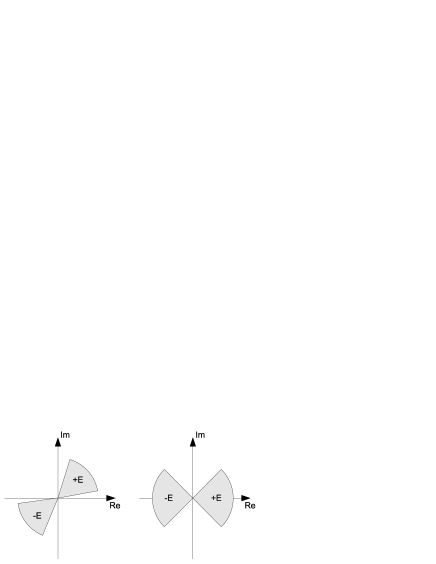
Figure 1: Eigenvalues of DTQW evolution operator on the complex plane. $+E$ and $-E$ denotes the regions of positive and negative energy respectively.

For the Hadamard walk, the both angles are $\pi/2$. The region of complex unit circle not covered by $\lambda_{\pm}(k)$ might be thought of as a forbidden region. One sees that the above properties make DTQW and the Dirac Equation alike.

The continuous limit of DTQW, both in time and space, has been studied in Refs. Asl (2004); Bracken (2006); Str1 (2006). It was shown that the continuous version of DTQW gives the evolution similar to the one described by the one-dimensional Dirac equation and that both models give the typical two horn probability distribution for initially highly localized wave packets. Aslangul Asl (2004) has studied the model with a coin of an arbitrary dimension with the coin operator being rotation of spin about $y$ axis, so the exact comparison with the Dirac equation cannot be made, although the models seems alike. It is also important to notice that the coin operator makes DTQW to be more general than the Dirac equation. In our case it can be an arbitrary $2\times 2$ unitary matrix. Due to this fact, the continuous version of DTQW must not always be Lorentz invariant. This is the case of the Hadamard walk.

Now, we will do something opposite to what was done in Refs. Asl (2004); Bracken (2006); Str1 (2006). Let us discretize Eq. (1) and see if it gives Eq. (4). We take $\sigma_{i}$ and $\sigma_{j}$ to be the $z$ and $y$ Pauli matrices respectively and use the same time symmetric procedure as in Ref. Wess (1999). We obtain a recursive formula that conserves probability to the second order in $\Delta t$:

$$\psi_{{~{}}_{d}^{u}}(x,t+\Delta t)=\frac{1-\gamma^{2}}{1+\gamma^{2}}\psi_{{~{}}_{d}^{u}}(x\mp\Delta x,t)\mp\frac{2\gamma}{1+\gamma^{2}}\psi_{{~{}}_{u}^{d}}(x,t),$$ (6)

where $\gamma=m\Delta t/2$. This looks similar to Eq. (4), but to make it more alike one should shift the right hand side of Eq. (6) by $l=\Delta x/2$ with the conditional translation operator $T$, Eq. (2). It means that DTQW is the discretized Dirac evolution viewed in, somehow strange, conditional moving reference frame. Note, that this shift does not occur when one considers the continuous limit of DTQW. This is due to the fact that in the continuous limit the differences between $U=TC$ and $U=CT$ vanishes because $C$ and $T$ act simultaneously. In the discrete regime it is important wether we act with $TC$ or $CT$. One can also easily check, that in the case $U=CT$, the left hand side of Eq. (6) should be shifted with the operator $T^{\dagger}$ in order to resemble the DTQW recursive formula. Also, choosing $\sigma_{i}$ and $\sigma_{j}$ to be different than here, gives the same effect. One also needs to remember that since DTQW is by definition discrete in space and time, it should be rather compared with the discrete Dirac equation than with its continuous more common version. It is due to the effects like Bloch oscillations My (2003) caused by discrete space and perhaps due to the other effects, yet unknown, related to discrete time.

Klein’s paradox and Zitterbewegung are effects that were first observed for the Dirac equation (for reference, look for example Ref. Sakurai (1967)). The first one is transfer of the particle with energy $E$ from the region with zero potential to the region with potential $V>V-m>E$ (see Fig.2).

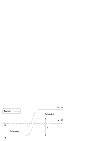
Figure 2: Klein’s paradox. The forbidden region $-m<E<m$ is shifted by a potential $V$. The particle with positive energy E is transferred to the negative energy region. The wave function of particle is not damped in the new region.

In relativistic case the wave function is not damped inside the potential region, unlike the solutions of the Schrödinger equation. The second effect is the rapid oscillation of a wave packet due to interference of its positive and negative energy components.

To observe Klein’s paradox in DTQW, one has to introduce a potential $V$. For simplicity, we take the step potential: all over the region $x>a$ the potential is $V_{0}$ and in the region $x\leq a$ the potential is zero. Adding the uniform potential simply shifts the energy $E^{\prime}=E+V_{0}$ and in the exponential form it may be written as $e^{-iE^{\prime}\Delta t}=e^{-i(E+V_{0})\Delta t}=e^{-iE\Delta t}e^{i\varphi}$. From now on, we will identify the potential with $e^{i\varphi}$. This will be very helpful to describe the existence of Klein’s paradox in DTQW in geometric way.

The eigenvalues without the potential are presented in Fig.3 a. In the presence of the potential, the eigenvalues are rotated by the angle $\varphi$, see Fig.3 b.

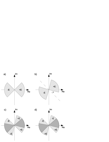
Figure 3: Eigenvalues of DTQW evolution operator on the complex plane: a) eigenvalues without potential, b) the same eigenvalues in the presence of a potential $e^{i\varphi}$, c) intersection of the eigenvalues of two regions, one without potential and one with the potential $e^{i\varphi}$, giving non decaying wave functions (dark grey), d) intersection of the eigenvalues of two regions, one without potential and one with the potential $e^{i(\varphi+\pi)}$, giving non decaying wave functions and leading to Klein’s paradox (dark grey).

Imagine that DTQW starts in the region without the potential and that there is a wave packet heading for the potential step $e^{i\varphi}$. The transmitted part of the wave packet may behave in two distinct ways: either move further without damping, or start to decay exponentially fast. Whether it is the first or the second case, depends directly on the eigenfunction decomposition of the wave packet. Let $\{\lambda\}_{0}$ denote the set of the eigenvalues of DTQW with no potential and $\{\lambda\}_{\varphi}$ be the set of the eigenvalues in the presence of the potential. Moreover, let $\{\lambda\}_{wp}\subset\{\lambda\}_{0}$ be the set of the eigenvalues which correspond to the eigenfunctions that contribute to the initial wave packet. By calculating $\{\lambda\}_{wp}\cap\{\lambda\}_{\varphi}$ one obtains the part of the wave packet that will not undergo damping. Now, let us study how this depends on $\varphi$. For small $\varphi$ the wave packet is not damped if its energy is higher than the potential step, similarly as in non-relativistic quantum mechanics, see Fig.3 c. As $\varphi$ rises, more eigenvalues fall into the forbidden region and the corresponding eigenfunctions are damped, until $\varphi$ is large enough and the eigenvalues from the cone $E_{+}$($E_{-}$) intersect with the eigenvalues of the rotated cone $E_{-}$($E_{+}$) (Fig.3 d). This is exactly Klein’s paradox. We should also point out that for specific coins, namely for the coins which make the eigenvalues cone dilation angle less or equal to $\pi/2$, one can choose a potentials that damp all eigenfunctions. The Hadamard walk is always damped in the potential region if $\varphi=\pi/2$. This might be useful if one would like to confine DTQW to some region. For example, it is possible to study the quantum walk on the line with one or two reflecting walls.

Zitterbewegung oscillation are expected to occur in both position and velocity. To measure this effect, we calculate how the position changes with the one step $\Delta X=X(t+\Delta t)-X(t)$. This is the discrete version of velocity. In the Heisenberg picture this might be written as $\Delta X=U^{\dagger}XU-X$, where $X=\sum_{x}x|x\rangle\langle x|$ and $U=TC$, as before. This leads us to the position independent coin operator

$$\Delta X=\left(\begin{array}[]{l}~{}|\alpha_{+}|^{2}-|\beta_{-}|^{2}~{}~{}~{}~{}~{}~{}\alpha_{+}^{\ast}\beta_{+}-\alpha_{-}\beta_{-}^{\ast}\\ \alpha_{+}\beta_{+}^{\ast}-\alpha_{-}^{\ast}\beta_{-}~{}~{}~{}~{}~{}~{}|\beta_{+}|^{2}-|\alpha_{-}|^{2}\end{array}\right).$$ (7)

To calculate its time dependence, we perform the discrete Fourier transform on the initial state and use the momentum representation to derive the expectation value of $\Delta X$ as a function of time. Calculation of DTQW probability distribution via Fourier transform was presented by Nayak and Vishwanath Nayak (2000). The general form of the time dependent wave function in momentum representation is

$$\tilde{\psi}(k,t)=\sum_{j=\pm}f_{j}(k)(\lambda_{j}(k))^{t}|c_{j}(k)\rangle,$$ (8)

where $f_{\pm}(k)$ are any square integrable functions obeying $\int_{-\pi}^{+\pi}dk(|f_{+}(k)|^{2}+|f_{-}(k)|^{2})=1$, and $|c_{\pm}(k)\rangle$, $\langle c_{\mp}(k)|c_{\pm}(k)\rangle=0$ are the coin states corresponding to the eigenvalues $\lambda_{\pm}(k)$. Since $\langle c_{-}(k)|\Delta X|c_{+}(k)\rangle=\langle c_{+}(k)|\Delta X|c_{-}(k)\rangle^{\ast}=g(k)$, the expectation value of $\Delta X(t)$ may be written as $A+B(t)$, where $A$ is a constant corresponding to the uniform velocity of the wave packet, and $B(t)$ is a time dependent term

$$B(t)=\int_{-\pi}^{+\pi}dk\left(f_{+}^{\ast}(k)f_{-}(k)g(k)(\lambda_{+}^{\ast}(k)\lambda_{-}(k))^{t}+c.c.\right).$$ (9)

The above vanish if the initial wave packet consists only of the positive or the negative energy eigenfunctions. As before, one may write the eigenvalues in the exponential form $\lambda_{\pm}(k)=e^{-i\varphi_{\pm}(k)}=e^{-iE_{\pm}(k)\Delta t}$, so the time dependent part under integral, Eq. (9), yields

$$(\lambda_{+}^{\ast}(k)\lambda_{-}(k))^{t}=e^{i(E_{+}(k)-E_{-}(k))t},$$ (10)

which has the form of oscillations. If we take the initial wave packet largely spread over the position space (for example broad Gaussian packet) and multiply it by the factor $e^{ik_{0}x}$, the corresponding momentum wave packet would be mainly localized around $k_{0}$. In this case Eq. (9) can be approximated by

$$B(t)\approx B\cos\left((E_{+}(k_{0})-E_{-}(k_{0}))t\right),$$ (11)

where $B$ is a time independent amplitude of oscillations. Of course, time is discrete and $t=n\Delta t$.

Zitterbewegung is very well visible if one chooses the standing wave packet, what in the case of DTQW does not always mean $k_{0}=0$. It is visible if one calculates the group velocity

$$v_{\pm}(k)=\frac{\partial E_{\pm}}{\partial k}=\frac{i}{\Delta t}\lambda_{\pm}^{\ast}(k)\frac{\partial\lambda_{\pm}(k)}{\partial k}.$$ (12)

Without loosing generality we assume $\Delta t=1$ and obtain

$$v_{\pm}(k)=\pm\frac{n_{z}\sin{\frac{\theta}{2}}\cos{k}-\cos{\frac{\theta}{2}}\sin{k}}{\sqrt{1-(\cos{\frac{\theta}{2}}\cos{k}+n_{z}\sin{\frac{\theta}{2}}\sin{k})^{2}}}.$$ (13)

Since the wave packet represents particle which does not move, $(E_{+}(k_{0})-E_{-}(k_{0}))\Delta t$ has the meaning of the mass. This result is closely related to the one of the Dirac equation with the oscillation frequency approximating $2m$. For the Hadamard walk, $v_{\pm}(k_{0})=0$ for $k_{0}=\pi/2$ and $\lambda_{\pm}(k_{0})=\frac{1\pm i}{\sqrt{2}}$, thus $(E_{+}(k_{0})-E_{-}(k_{0}))\Delta t=\pi/2$.

The presence of Klein’s paradox and Zitterbewegung in DTQW leads to the bunch of questions. First of all, are the two effects truly relativistic, since DTQW might be implemented with non-relativistic quantum mechanics? The implementations of DTQW has been presented for various physical systems, from optical latices to trapped ions Dur (2002); Joo (2006); Hillery (2003); Jeong (2004); Eckert (2005); Trav (2002), just to point some of them. One may even think of the Stern-Gerlach experiment as of a quantum quincunx with the magnetic field along $x$ and $z$ axes at even and odd time steps respectively. The implementation schemes might be different, but it is worth to notice that none of them has anything to do with the Dirac equation. Of course one may wonder if it is right to consider such concepts like spin and talk about non-relativistic quantum physics, but the fact is that we may include spin in the non-relativistic Schrödinger equation without bothering about its origin. Moreover, this equation would correctly predict the behavior of a real system.

In conclusion, effects associated with relativistic quantum mechanics were shown to appear in non-relativistic models. We derived formula for Zitterbewegung oscillations, Eq. (11), and presented in graphical way the nature of Klein’s paradox. DTQW was also compared with the discrete Dirac equation and it was shown that the two models are related to each other and that one may go from one to another by changing the reference frame.

The author would like to thank Michał Kurzyński, Antoni Wójcik and Andrzej Grudka for their kind help, stimulating conversations and pointing important references.

References

- Ahar (1993) Y. Aharonov, L. Davidovich, and N. Zagury, Phys. Rev. A, 48, 1687 (1993).
- Farhi (1998) E. Farhi and S. Gutmann, Phys. Rev. A, 58, 915 (1998).
- Kempe (2003) J. Kempe, Contemp. Phys., 44, 307 (2003).
- Ambainis (2004) A. Ambainis, quant-ph/0403120.
- Wojc (2003) D.K. Wójcik and J.R. Dorfman, Phys. Rev. Lett., 90, 230260 (2003).
- My (2003) A. Wójcik, T. Łuczak, P. Kurzyński, A. Grudka and M. Bednarska, Phys. Rev. Lett., 93, 180601 (2004).
- Str1 (2006) F.W. Strauch, Phys. Rev. A, 73, 054302 (2006).
- Bracken (2006) A.J. Bracken, D. Ellinas, and I. Smyrnakis, quant-ph/06105195.
- Fynmann (1965) R.P. Feynmann and A.R. Hibbs, Quantum Mechanics and Path Integrals, McGraw-Hill, New York (1965).
- Asl (2004) C. Aslangul, quant-ph/0406057.
- Wess (1999) P.P.F. Wessels, W.J. Caspers, and F.W. Wiegel, Europhys. Lett., 46(2), 123-126 (1999).
- Sakurai (1967) J.J. Sakurai, Advanced Quantum Mechanics, Addison-Wesley (1967).
- Nayak (2000) A. Nayak and A. Vishwanath, quant-ph/0010117.
- Dur (2002) W. Dür, R. Raussendorf, V.M. Kendon and H.-J. Briegel, Phys. Rev. A, 66, 052319 (2002).
- Joo (2006) J. Joo, P.L. Knight and J.K. Pachos, quant-ph/0606087.
- Hillery (2003) M. Hillery, J. Bergou and E. Feldman, quant-ph/0302161.
- Jeong (2004) H. Jeong, M. Paternostro and M.S. Kim, Phys. Rev. A, 69, 012310 (2004).
- Eckert (2005) K. Eckert, J. Mompart, G. Birkl and M Lewenstein, Phys. Rev. A, 72, 012327 (2005).
- Trav (2002) B.C. Travaglione and G.J. Milburn, Phys. Rev. A, 65, 032310 (2002).