A First-Principles Method for Open Electronic Systems

Abstract

We prove that the electron density function of a real physical system can be uniquely determined by its values on any finite subsystem. This establishes the existence of a rigorous density-functional theory for any open electronic system. By introducing a new density functional for dissipative interactions between the reduced system and its environment, we subsequently develop a time-dependent density-functional theory which depends in principle only on the electron density of the reduced system. In the steady-state limit, the conventional first-principles nonequilibrium Green’s function formulation for the current is recovered. A practical scheme is proposed for the new density functional: the wide-band limit approximation, which is applied to simulate the transient current through a model molecular device.

I Introduction

Density-functional theory (DFT) has been widely used as a research tool in condensed matter physics, chemistry, materials science, and nanoscience. The Hohenberg-Kohn theorem hk lays the foundation of DFT. The Kohn-Sham formalism ks provides a practical solution to calculate the ground state properties of electronic systems. Runge and Gross extended DFT further to calculate the time-dependent properties and hence the excited state properties of any electronic systems tddft . The accuracy of DFT or time-dependent DFT (TDDFT) is determined by the exchange-correlation (XC) functional. If the exact XC functional were known, the Kohn-Sham formalism would have provided the exact ground state properties, and the Runge-Gross extension, TDDFT, would have yielded the exact time-dependent and excited states properties. Despite their wide range of applications, DFT and TDDFT have been mostly limited to isolated systems.

Many systems of current research interest are open systems. A molecular electronic device is one such system. DFT-based simulations have been carried out on such devices prllang ; prlheurich ; jcpluo ; langprb ; prbguo ; jacsywt ; jacsgoddard ; transiesta ; jcpratner . These simulations focus on steady-state currents under bias voltages. Two types of approaches have been adopted. One is the Lippmann-Schwinger formalism by Lang and coworkers langprb . The other is the first-principles nonequilibrium Green’s function (NEGF) technique prbguo ; jacsywt ; jacsgoddard ; transiesta ; jcpratner . In both approaches the Kohn-Sham Fock operator is taken as the effective single-electron model Hamiltonian, and the transmission coefficients are calculated within the noninteracting electron model. The investigated systems are not in their ground states, and applying ground state DFT formalism for such systems is only an approximation cpdatta . DFT formalisms adapted for current-carrying systems have also been proposed recently, such as Kosov’s Kohn-Sham equations with direct current jcpkosov and Burke et al.’s Kohn-Sham master equation including dissipation to phonons prlburke . However, practical implementation of these formalisms requires the electron density function of the entire system. In this paper, we present a rigorous DFT formalism for open electronic systems, and use it to simulate the steady and transient currents through molecular electronic devices. The first-principles formalism depends only on the electron density function of the reduced system.

This paper is organized as follows. In Sec. II we propose a TDDFT formalism for open electronic systems based on the equation of motion (EOM) for reduced single-electron density matrix. In Sec. III we prove the theorem that the electron density function of any finite subsystem can determine uniquely all properties of a connected real physical system. By utilizing this theorem we introduce in Sec. IV a dissipation functional for the electron density of the subsystem, and thus establish a rigorous and efficient first-principles formalism for steady and transient dynamics of open electronic systems. An wide-band limit (WBL) approximation scheme for the dissipation functional is proposed for practical implementations in Sec. V. To demonstrate the applicability of our first-principles formalism, a TDDFT calculation is carried out to simulate the transient current through a model molecular device. The detailed procedures and results are described in Sec. VI. Discussion and summary are given in Sec. VII.

II First-principles formalism

II.1 Reduced single-electron density matrix and TDDFT formalism for reduced system

Fig. 1 depicts an open electronic system. Region $D$ is the reduced system of our interests, and the electrodes $L$ and $R$ are the environment. Altogether $D$, $L$ and $R$ form the entire system. Taking Fig. 1 as an example, we develop a practical DFT formalism for the open systems. Within the TDDFT formalism, a closed EOM has been derived for the reduced single-electron density matrix $\sigma(t)$ of the entire system ldmtddft :

$$i\dot{\sigma}(t)=[h(t),\sigma(t)],$$ (1)

where $h(t)$ is the Kohn-Sham Fock matrix of the entire system, and the square bracket on the right-hand side (RHS) denotes a commutator. The matrix element of $\sigma$ is defined as $\sigma_{ij}(t)=\langle a^{\dagger}_{j}(t)\,a_{i}(t)\rangle$, where $a_{i}(t)$ and $a^{\dagger}_{j}(t)$ are the annihilation and creation operators for atomic orbitals $i$ and $j$ at time $t$, respectively. Fourier transformed into frequency domain while considering linear response only, Eq. (1) leads to the conventional Casida’s equation casida . Expanded in the atomic orbital basis set, the matrix representation of $\sigma$ can be partitioned as

$$\sigma=\left[\begin{array}[]{lll}\sigma_{L}&\sigma_{LD}&\sigma_{LR}\\ \sigma_{DL}&\sigma_{D}&\sigma_{DR}\\ \sigma_{RL}&\sigma_{RD}&\sigma_{R}\end{array}\right],$$ (2)

where $\sigma_{L}$, $\sigma_{R}$ and $\sigma_{D}$ represent the diagonal blocks corresponding to the left lead $L$, the right lead $R$ and the device region $D$, respectively; $\sigma_{LD}$ is the off-diagonal block between $L$ and $D$; and $\sigma_{RD}$, $\sigma_{LR}$, $\sigma_{DL}$, $\sigma_{DR}$ and $\sigma_{RL}$ are similarly defined. The Kohn-Sham Fock matrix $h$ can be partitioned in the same way with $\sigma$ replaced by $h$ in Eq. (2). Thus, the EOM for $\sigma_{D}$ can be written as

$$i\dot{\sigma}_{D} = [h_{D},\sigma_{D}]+\sum_{\alpha=L,R}\left(h_{D\alpha}\sigma_{\alpha D}-\sigma_{D\alpha}h_{\alpha D}\right)$$ (3)

$$= [h_{D},\sigma_{D}]-i\sum_{\alpha=L,R}Q_{\alpha},$$

where $Q_{L}$ ($Q_{R}$) is the dissipative term due to $L$ ($R$). With the reduced system $D$ and the leads $L/R$ spanned respectively by atomic orbitals $\{l\}$ and single-electron states $\{k_{\alpha}\}$, Eq. (3) is equivalent to:

$$i\dot{\sigma}_{nm} = \sum_{l\in D}\,(h_{nl}\sigma_{lm}-\sigma_{nl}h_{lm})-i\sum_{\alpha=L,R}Q_{\alpha,nm},$$ (4)

$$Q_{\alpha,nm} = i\sum_{k_{\alpha}\in\alpha}\big{(}h_{nk_{\alpha}}\sigma_{k_{\alpha}m}-\sigma_{nk_{\alpha}}h_{k_{\alpha}m}\big{)},$$ (5)

where $m$ and $n$ correspond to the atomic orbitals in region $D$; $k_{\alpha}$ corresponds to an electronic state in the electrode $\alpha$ ($\alpha=L$ or $R$). $h_{nk_{\alpha}}$ is the coupling matrix element between the atomic orbital $n$ and the electronic state $k_{\alpha}$. The current through the interfaces $S_{L}$ or $S_{R}$ (see Fig. 1) can be evaluated as follows,

$$J_{\alpha}(t) = -\int_{\alpha}d\mathbf{r}\,\frac{\partial}{\partial t}\rho(\mathbf{r},t)$$ (6)

$$= -\sum_{k_{\alpha}\in\alpha}\frac{d}{dt}\,\sigma_{k_{\alpha}k_{\alpha}}\!(t)$$

$$= i\sum_{l\in D}\sum_{k_{\alpha}\in\alpha}\big{(}h_{k_{\alpha}l}\,\sigma_{lk_{\alpha}}-\sigma_{k_{\alpha}l}\,h_{lk_{\alpha}}\big{)}$$

$$= -\sum_{l\in D}Q_{\alpha,ll}=-\mbox{tr}\big{[}Q_{\alpha}(t)\big{]},$$

i.e., the trace of $Q_{\alpha}$.

II.2 Solution for steady-state current

Based on the Keldysh formalism keldysh and the analytic continuation rules of Langreth langreth , $Q_{\alpha,nm}(t)$ can be calculated by the NEGF formulation as described in Reference prb94win (see Appendix A)

$$Q_{\alpha,nm}(t) = -\sum_{l\in D}\int_{-\infty}^{\infty}d\tau\Big{[}\,G^{<}_{nl}(t,\tau)\Sigma^{a}_{\alpha,lm}(\tau,t)+$$ (7)

$$\,G^{r}_{nl}(t,\tau)\Sigma^{<}_{\alpha,lm}(\tau,t)-\Sigma^{<}_{\alpha,nl}(t,\tau)G^{a}_{lm}(\tau,t)$$

$$-\,\Sigma^{r}_{\alpha,nl}(t,\tau)G^{<}_{lm}(\tau,t)\Big{]},$$

where $G^{r}$, $G^{a}$ and $G^{<}$ are the retarded, advanced and lesser Green’s function for the reduced system $D$, respectively, and $\Sigma^{r}_{\alpha}$, $\Sigma^{a}_{\alpha}$ and $\Sigma^{<}_{\alpha}$ are the retarded, advanced and lesser self-energies due to the lead $\alpha$ ($L$ or $R$), respectively. Combining Eqs. (6) and (7), we obtain

$$J_{\alpha}(t) = 2\Re\,\bigg{\{}\int_{-\infty}^{\infty}\!d\tau\,\,\mbox{tr}\Big{[}G^{<}_{D}(t,\tau)\Sigma^{a}_{\alpha}(\tau,t)+$$ (8)

$$G^{r}_{D}(t,\tau)\Sigma^{<}_{\alpha}(\tau,t)\Big{]}\bigg{\}}.$$

The same expression was derived by Stefanucci and Almbladh within the framework of TDDFT qttddft .

It is important to point out that Eqs. (1)$-$(5) follow the partition-free scheme proposed by Cini cini , while Eq. (7) was derived if one follows the partitioned scheme developed by Caroli et al. caroli . In the above derivation we assume that the equivalence of the two schemes, which is satisfied if the two self-energies behave asymptotically as follows qttddft ,

$$\lim_{t\rightarrow\infty}\Sigma^{r}_{\alpha}(t,t^{\prime})=\lim_{t\rightarrow\infty}\Sigma^{a}_{\alpha}(t^{\prime},t)=0.$$ (9)

As $t,\tau\rightarrow+\infty$, $\Gamma^{k_{\alpha}}_{nm}(t,\tau)=h_{nk_{\alpha}}(t)\,h_{k_{\alpha}m}(\tau)$ becomes asymptotically time-independent. The Green’s functions for the reduced system $D$ rely simply on the difference of the two time-variables qttddft , and can thus be expressed as

$$G^{<}_{nm}(t,\tau) = \sum_{p,q\in D}\int_{-\infty}^{\infty}dt_{1}\int_{-\infty}^{\infty}dt_{2}\,G^{r}_{np}(t,t_{1})$$ (10)

$$\times\,\Sigma^{<}_{pq}(t_{1},t_{2})\,G^{a}_{qm}(t_{2},\tau)$$

$$= i\sum_{p,q\in D}\sum_{\alpha=L,R}\sum_{l_{\alpha}\in\alpha}f^{\alpha}_{l}$$

$$\times\left[\int_{-\infty}^{\infty}dt_{1}\textnormal{e}^{-i\epsilon_{l}^{\alpha}t_{1}}G^{r}_{np}(t-t_{1})\right]\Gamma^{l_{\alpha}}_{pq}$$

$$\times\left[\int_{-\infty}^{\infty}dt_{2}\textnormal{e}^{i\epsilon_{l}^{\alpha}t_{2}}G^{a}_{qm}(t_{2}-\tau)\right]$$

$$= i\sum_{p,q\in D}\sum_{\alpha=L,R}\sum_{l_{\alpha}\in\alpha}f^{\alpha}_{l}\textnormal{e}^{-i\epsilon^{\alpha}_{l}(t-\tau)}$$

$$\times\,G^{r}_{np}(\epsilon^{\alpha}_{l})\,\Gamma^{l_{\alpha}}_{pq}\,G^{a}_{qm}(\epsilon^{\alpha}_{l}),$$

$$G^{r,a}_{nm}(\epsilon) = \left[\epsilon I-h-\Sigma^{r,a}(\epsilon)\right]^{-1}_{nm},$$ (11)

$$\Sigma^{r,a}_{nm}(\epsilon) = \sum_{\alpha=L,R}\sum_{l\in\alpha}\,\Gamma^{l_{\alpha}}_{nm}\left(\epsilon-\epsilon_{l}^{\alpha}\pm i\Delta\right)^{-1},$$ (12)

where $I$ is the identity matrix. The steady-state current can thus be explicitly expressed by combining Eqs. (10)$-$(12),

$$J_{L}(\infty) = -J_{R}(\infty)$$ (13)

$$= -\sum_{n\in D}Q_{L,nn}(\infty)$$

$$= 2\pi\,\Bigg{\{}\sum_{k\in L}f^{L}_{k}\sum_{l\in R}\Delta(\epsilon^{R}_{l}-\epsilon^{L}_{k})$$

$$\times\,\mbox{tr}\Big{[}G^{r}_{D}(\epsilon^{L}_{k})\,\Gamma^{l_{R}}\,G^{a}_{D}(\epsilon^{L}_{k})\,\Gamma^{k_{L}}\Big{]}$$

$$-\sum_{l\in R}f^{R}_{l}\sum_{k\in L}\delta(\epsilon^{L}_{k}-\epsilon^{R}_{l})$$

$$\times\,\mbox{tr}\Big{[}G^{r}_{D}(\epsilon^{R}_{l})\,\Gamma^{l_{R}}\,G^{a}_{D}(\epsilon^{R}_{l})\,\Gamma^{k_{L}}\Big{]}\Bigg{\}}$$

$$= \int\left[f^{L}(\epsilon)-f^{R}(\epsilon)\right]T(\epsilon)\,d\epsilon,$$

$$T(\epsilon) = 2\pi\,\eta_{L}\eta_{R}\,\mbox{tr}\Big{[}G^{r}_{D}(\epsilon)\Gamma^{R}(\epsilon)G^{a}_{D}(\epsilon)\Gamma^{L}(\epsilon)\Big{]}.$$ (14)

Here $T(\epsilon)$ is the transmission coefficient, $f^{\alpha}(\epsilon)$ is the Fermi distribution function, and $\eta_{\alpha}(\epsilon)=\sum_{k\in\alpha}\delta(\epsilon-\epsilon^{\alpha}_{k})$ is the density of states (DOS) for the lead $\alpha$ ($L$ or $R$). Eq. (13) is exactly the Landauer formula bookdatta ; landauer in the DFT-NEGF formalism prbguo ; jacsywt . The difficulty in solving Eq. (4) is to calculate $Q_{\alpha,nm}$. Employing the Keldysh NEGF formalism, the evaluation of $Q_{\alpha,nm}$ involves the calculation of two-time Green’s functions and self-energies as those appearing in Eq. (7), which makes the simulation of any real molecular device computationally impractical. An alternative approach must be developed.

III Holographic electron density theorem for time-dependent systems

As early as in 1981, Riess and Münch riess discovered the holographic electron density theorem which states that any nonzero volume piece of the ground state electron density determines the electron density of a molecular system. This is based on that the electron density functions of atomic and molecular eigenfunctions are real analytic away from nuclei. In 1999 Mezey extended the holographic electron density theorem mezey . And in 2004 Fournais et al. proved again the real analyticity of the electron density functions of any atomic or molecular eigenstates analyticity . Therefore, for a time-independent real physical system made of atoms and molecules, its electron density function is real analytic (except at nuclei) when the system is in its ground state, any of its excited eigenstates, or any state which is a linear combination of finite number of its eigenstates; and the ground state electron density on any finite subsystem determines completely the electronic properties of the entire system.

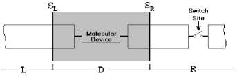
Figure 1: Schematic representation of the experimental setup for quantum transport through a molecular device.

As for time-dependent systems, the issue is less clear. Although it seems intuitive that the electron density function of any time-dependent real physical system is real analytic (except for isolated points in space-time), it turns out quite difficult to prove the analyticity rigorously. Fortunately we are able to establish a one-to-one correspondence between the electron density function of any finite subsystem and the external potential field which is real analytic in both $t$-space and $\mathbf{r}$-space, and thus circumvent the difficulty concerning the analyticity of time-dependent electron density function. For time-dependent real physical systems, we have the following theorem:

Theorem: If the electron density function of a real physical system at $t_{0}$, $\rho(\mathbf{r},t_{0})$, is real analytic in $\mathbf{r}$-space, the corresponding wave function is $\Phi(t_{0})$, and the system is subjected to a real analytic (in both $t$-space and $\mathbf{r}$-space) external potential field $v(\mathbf{r},t)$, the time-dependent electron density function on any finite subspace $D$, $\rho_{D}(\mathbf{r},t)$, has a one-to-one correspondence with $v(\mathbf{r},t)$ and determines uniquely all electronic properties of the entire time-dependent system.

Proof: Let $v(\mathbf{r},t)$ and $v^{\prime}(\mathbf{r},t)$ be two real analytic potentials in both $t$-space and $\mathbf{r}$-space which differ by more than a constant at any time $t\geqslant t_{0}$, and their corresponding electron density functions are $\rho(\mathbf{r},t)$ and $\rho^{\prime}(\mathbf{r},t)$, respectively. Therefore, there exists a minimal nonnegative integer $k$ such that the $k$-th order derivative differentiates these two potentials at $t_{0}$:

$$\left.\frac{\partial^{k}}{\partial t^{k}}\left[v(\mathbf{r},t)-v^{\prime}(\mathbf{r},t)\right]\right|_{t=t_{0}}\neq\mbox{const}.$$ (15)

Following exactly the Eqs. (3)-(6) of Ref. tddft , we have

$$\left.\frac{\partial^{k+2}}{\partial t^{k+2}}\left[\rho(\mathbf{r},t)-\rho^{\prime}(\mathbf{r},t)\right]\right|_{t=t_{0}} = -\nabla\cdot u(\mathbf{r}),$$ (16)

where

$$u(\mathbf{r}) = \rho(\mathbf{r},t_{0})\,\nabla\!\left\{\left.\frac{\partial^{k}}{\partial t^{k}}\left[v(\mathbf{r},t)-v^{\prime}(\mathbf{r},t)\right]\right|_{t=t_{0}}\right\}.$$ (17)

Due to the analyticity of $\rho(\mathbf{r},t_{0})$, $v(\mathbf{r},t)$ and $v^{\prime}(\mathbf{r},t)$, $\nabla\cdot u(\mathbf{r})$ is also real analytic in $\mathbf{r}$-space. It has been proven in Ref. tddft that it is impossible to have $\nabla\cdot u(\mathbf{r})=0$ on the entire $\mathbf{r}$-space. Therefore it is also impossible that $\nabla\cdot u(\mathbf{r})=0$ everywhere in $D$ because of analytical continuation of $\nabla\cdot u(\mathbf{r})$. Note that $\rho_{D}(\mathbf{r},t)=\rho(\mathbf{r},t)$ for $\mathbf{r}\in D$. We have thus

$$\left.\frac{\partial^{k+2}}{\partial t^{k+2}}\left[\rho_{D}(\mathbf{r},t)-\rho_{D}^{\prime}(\mathbf{r},t)\right]\right|_{t=t_{0}} \neq 0$$ (18)

for $\mathbf{r}\in D$. This confirms the existence of a one-to-one correspondence between $v(\mathbf{r},t)$ and $\rho_{D}(\mathbf{r},t)$. $\rho_{D}(\mathbf{r},t)$ thus determines uniquely all electronic properties of the entire system. This completes the proof of the Theorem.

Note that if $\Phi(t_{0})$ is the ground state, any excited eigenstate, or any state as a linear combination of finite number of eigenstates of a time-independent Hamiltonian, the prerequisite condition in Theorem that the electron density function $\rho(\mathbf{r},t_{0})$ be real analytic is automatically satisfied, as proven in Ref. analyticity . As long as the electron density function at $t=t_{0}$, $\rho(\mathbf{r},t_{0})$, is real analytic, it is guaranteed that $\rho_{D}(\mathbf{r},t)$ of the subsystem $D$ determines all physical properties of the entire system at any time $t$ if the external potential $v(\mathbf{r},t)$ is real analytic.

According to the above Theorem, the electron density function of any subsystem determines all the electronic properties of the entire time-dependent physical system. This proves in principle the existence of a rigorous DFT-type formalism for open electronic systems. All one needs to know is the electron density of the reduced system.

IV Dissipative density functional

According to the holographic electron density theorem of time-dependent physical systems, all physical quantities are explicit or implicit functionals of the electron density in the reduced system $D$, $\rho_{D}(\mathbf{r},t)$. $Q_{\alpha}$ of Eq. (3) is thus also a universal functional of $\rho_{D}(\mathbf{r},t)$. Therefore, Eq. (4) can be recast into a formally closed form,

$$\!\!i\dot{\sigma_{D}}=\Big{[}h_{D}[\mathbf{r},t;\rho_{D}(\mathbf{r},t)],\sigma_{D}\Big{]}-i\!\!\sum_{\alpha=L,R}\!\!Q_{\alpha}[\mathbf{r},t;\rho_{D}(\mathbf{r},t)].$$ (19)

Neglecting the second term on the RHS of Eq. (19) leads to the conventional TDDFT formulation in terms of reduced single-electron density matrix ldmtddft for the isolated reduced system. The second term describes the dissipative processes between $D$ and $L$ or $R$. Besides the XC functional, an additional universal density functional, the dissipation functional $Q_{\alpha}[\mathbf{r},t;\rho_{D}(\mathbf{r},t)]$, is introduced to account for the dissipative interaction between the reduced system and its environment. Eq. (19) is the TDDFT EOM for open electronic systems. It would thus be much more efficient integrating Eq. (19) than solving Eqs. (4) and (7), if $Q_{\alpha}[\mathbf{r},t;\rho_{D}(\mathbf{r},t)]$ or its approximation is known. We therefore have a practical and potentially rigorous formalism for any open electronic systems. Burke et al. extended TDDFT to include electronic systems interacting with phonon baths prlburke , they proved the existence of a one-to-one correspondence between $v(\mathbf{r},t)$ and $\rho(\mathbf{r},t)$ under the condition that the dissipative interactions (denoted by a superoperator $\mathcal{C}$ in Ref. prlburke ) between electrons and phonons are fixed. In our case since the electrons can move in and out the reduced system, the number of the electrons in the reduced system is not conserved. In addition, the dissipative interactions can be determined in principle by the electron density of the reduced system. We do not need to stipulate that the dissipative interactions with the environment are fixed as Burke et al.. And the only information we need is the electron density of the reduced system. In the frozen DFT approach warshel an additional XC functional term was introduced to account for the XC interaction between the system and the environment. This additional term is included in $h_{D}[\mathbf{r},t;\rho_{D}(\mathbf{r},t)]$ of Eq. (19).

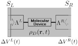
Figure 2: Schematic representation of the reduced system $D$ within the WBL scheme for dissipation functional $Q_{\alpha}$.

Given $Q_{\alpha}[\rho_{D}(\mathbf{r},t)]$ how do we solve the EOM (19) in practice? Again take the molecular device shown in Fig. 1 as an example. We focus on the reduced system $D$ as depicted in Fig. 2, and integrate the EOM (19) directly by satisfying the boundary conditions at $S_{L}$ and $S_{R}$. $\Delta V^{L}(t)$ and $\Delta V^{R}(t)$ are the bias voltages applied on $L$ and $R$, respectively, and serve as the boundary conditions at $S_{L}$ and $S_{R}$, respectively. At $t\rightarrow-\infty$, $\Delta V^{L}=\Delta V^{R}=0$, and near $t=0$ $\Delta V^{L}(t)$ and $\Delta V^{R}(t)$ are turned on adiabatically. We need thus integrate Eq. (19) together with a Poisson equation for Coulomb potential inside the device region $D$. And the Poisson equation is subjected to the boundary condition determined by the potentials at $S_{L}$ and $S_{R}$.

V Wide-band limit approximation for dissipation functional $\mathbf{Q}_{\mathbf{\alpha}}$ and its test on a model system

An explicit form for the dissipation functional $Q_{\alpha}$ is required for practical implementation of Eq. (19). Admittedly $Q_{\alpha}[\mathbf{r},t;\rho_{D}(\mathbf{r},t)]$ is an extremely complex functional and difficult to evaluate. As various approximated expressions have been adopted for the DFT XC functional in practical implementations, the same strategy can be applied to the dissipation functional $Q_{\alpha}$.

One such scheme is the wide-band limit (WBL) approximation prb94win which involves the following assumptions for the leads: (i) their band-widths are assumed to be infinitely large, (ii) their line-widths, $\Lambda^{\alpha}_{k}(t,\tau)$, defined by the DOS at $S_{L}$ or $S_{R}$ times the coupling strength between $D$ and $L$ or $R$, i.e., $\Lambda^{\alpha}_{k}(t,\tau)=\pi\,\eta_{\alpha}(\epsilon^{\alpha}_{k})\,\Gamma^{k_{\alpha}}(t,\tau)$, are treated as energy independent, i.e., $\Lambda^{\alpha}_{k}(t,\tau)\approx\Lambda^{\alpha}(t,\tau)\approx\Lambda^{\alpha}$, and (iii) the level shifts of $L$ or $R$ are taken as a constant for all energy levels, i.e., $\Delta\epsilon^{\alpha}_{k}(t)\approx\Delta\epsilon^{\alpha}(t)=-\Delta V^{\alpha}(t)$, where $\Delta V^{\alpha}(t)$ are bias voltages applied on $L$ or $R$ at time $t$. The detailed derivations for the WBL scheme can be found in Appendix B and the explicit form for $Q^{WBL}_{\alpha}$ is given here,

$$Q^{WBL}_{\alpha}(t)=K^{\alpha}(t)+\left\{\Lambda^{\alpha},\sigma_{D}(t)\right\},$$ (20)

Here $K^{\alpha}(t)$ is fully expanded as follows,

$$K^{\alpha}(t) = -\frac{2i}{\pi}\,\bigg{\{}\,U^{\alpha}(t)\int_{-\infty}^{\mu^{0}}\frac{d\epsilon\,\mbox{e}^{i\epsilon t}}{\epsilon-h_{D}(0)+i\,\Lambda}$$ (21)

$$+\int_{-\infty}^{\mu^{0}}\left[I-U^{\alpha}(t)\,\mbox{e}^{i\epsilon t}\right]$$

$$\times\frac{d\epsilon}{\epsilon-h_{D}(t)+i\,\Lambda+\Delta\epsilon^{\alpha}(t)}\bigg{\}}\Lambda^{\alpha}+H.C.$$

where

$$U^{\alpha}(t) = \mbox{e}^{-i\int_{0}^{t}\left[h_{D}(\tau)-i\Lambda-\Delta\epsilon^{\alpha}(\tau)\right]d\tau}.$$ (22)

From Eqs. (20)-(22) it is clear that the dissipation functional $Q_{\alpha}$ within WBL scheme depends explicitly on $\Delta\epsilon^{\alpha}(t)$, $\sigma_{D}(t)$, $h_{D}(t)$ and $\Lambda^{\alpha}$. Note that $\Delta\epsilon^{\alpha}(t)=-\Delta V^{\alpha}(t)$ and $\Delta V^{\alpha}(t)$ is a functional of $\rho_{D}(\mathbf{r},t)$, i.e., $\Delta V^{\alpha}(t)\equiv\Delta V^{\alpha}\left[\rho_{D}(\mathbf{r},t),t\right]$; $h_{D}(t)\equiv h_{D}\left[\sigma_{D}(t),t\right]$; since $\eta_{\alpha}(\epsilon)$ is the DOS at $S_{\alpha}$ ($\alpha=L$ or $R$), and $\Gamma^{\alpha}$ is the coupling strength between the surface states at $S_{\alpha}$ and the bulk states of $D$, $\Lambda^{\alpha}$ is thus a functional of $\rho_{D}(\mathbf{r},t)$, i.e., $\Lambda^{\alpha}\equiv\Lambda^{\alpha}\left[\rho_{D}(\mathbf{r},t),t\right]$. We hence conclude that in practice $Q^{WBL}_{\alpha}$ is a functional of $\rho_{D}(\mathbf{r},t)$, i.e.,

$$Q^{WBL}_{\alpha}(t) \equiv Q^{WBL}_{\alpha}\Big{[}\sigma_{D}\!\left[\rho_{D}\right],\,h_{D}[\sigma_{D}\!\left[\rho_{D}\right],t],$$ (23)

$$\Lambda^{\alpha}[\rho_{D},t],\,\Delta V^{\alpha}[\rho_{D},t],\,t\Big{]}.$$

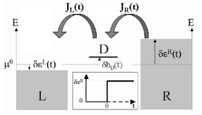
Figure 3: Model system for the test of the WBL dissipation functional where a single site spans the device region $D$. Transient currents through leads $L$ and $R$, $J_{L}(t)$ and $J_{R}(t)$, are simulated. The inset shows the time-dependent level shift of lead $R$.

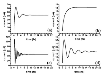
Figure 4: The calculated transient current through $S_{R}$ within the WBL scheme. We set $\mu^{0}=h_{D}(0)=0$ for the ground state; and $\Delta\epsilon^{L}(t)=0$ and $\Delta\epsilon^{R}(t)=\Delta\epsilon^{R}\,(1-\mbox{e}^{-t/a})$ after switch-on. The above panels show different cases where (a) $\Delta\epsilon^{R}=2$ eV, $\Lambda^{L}=\Lambda^{R}=0.1$ eV; (b) $\Delta\epsilon^{R}=0.2$ eV, $\Lambda^{L}=\Lambda^{R}=0.1$ eV; (c) $\Delta\epsilon^{R}=10$ eV, $\Lambda^{L}=\Lambda^{R}=0.1$ eV; and (d) $\Delta\epsilon^{R}=2$ eV, $\Lambda^{L}=\Lambda^{R}=0.04$ eV, respectively.

The WBL dissipation functional $Q^{WBL}_{\alpha}$ is then tested by calculations on a model system which has previously been investigated by Maciejko, Wang and Guo pulse2c . In this model system the device region $D$ consists of a single site spanned by only one atomic orbital (see Fig. 3). Exact transient current driven by a step voltage pulse has been obtained from NEGF simulations pulse2c , and the authors concluded that the WBL approximation yields reasonable results provided that the band-widths of the leads are five times or larger than the coupling strength between $D$ and $L$ or $R$. The computational details are as follows. The entire system ($L$ + $R$ + $D$) is initially in its ground state with the chemical potential $\mu^{0}$. External bias voltages are switched on from the time $t=0$, which results in transient current flows through the leads $L$ and $R$. $\delta h_{D}(t)\equiv h_{D}(t)-h_{D}(0)$, $\Delta\epsilon^{L}(t)$ and $\Delta\epsilon^{R}(t)$ are the level shifts of $D$, $L$ and $R$ at time $t$, respectively. In our works we take $\delta h_{D}(t)=\frac{1}{2}\left[\Delta\epsilon^{L}(t)+\Delta\epsilon^{R}(t)\right]$, $\Delta\epsilon^{L}(t)=0$, and $\Delta\epsilon^{R}(t)=\Delta\epsilon^{R}\,(1-\mbox{e}^{-t/a})$, where $a$ is a positive constant. The real analytic level shift $\Delta\epsilon^{R}(t)$ resembles perfectly a step pulse as $a\rightarrow 0^{+}$. The calculation results are demonstrated in Fig. 4. We choose exactly the same parameter set as that adopted for Fig. 2 in Ref. pulse2c , and the resulting transient current, represented by Fig. 4(a), excellently reproduces the WBL result in Ref. pulse2c , although the numerical procedures employed are distinctively different. The comparison confirms evidently the accuracy of our formalism. From Fig. 4(a)-(c) it is observed that with the same line-widths $\Lambda^{\alpha}$, a larger level shift $\Delta\epsilon^{R}$ results in a more fluctuating current, whereas by comparing (a) and (d) we see that under the same $\Delta\epsilon^{R}$, the current decays more rapidly to the steady state value with larger $\Lambda^{\alpha}$.

Since the integration over energy in Eq. (21) can be performed readily by transforming the integrand into diagonal representation, $Q^{WBL}_{\alpha}$ are evaluated efficiently, which makes the WBL scheme a practical routine for subsequent TDDFT calculations.

VI A TDDFT calculation of transient current

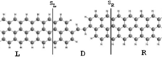
Figure 5: A two-dimensional model molecular device is connected to left and right leads.

With the EOM (19) and the WBL scheme for the dissipation functional $Q_{\alpha}$, it is now straightforward to carry out first-principles calculations for transient dynamics of open electronic systems. A model molecular device depicted in Fig. 5 is taken as the open system under investigation. The device region $D$ containing $24$ carbon and $12$ hydrogen atoms is spanned by the 6-31 Gaussian basis set, i.e., altogether $240$ basis functions for the reduced system. The leads are quasi-one-dimensional graphene sheets with dangling bonds saturated by hydrogen atoms, and the entire system is on a same plane. The ground state reduced single-electron density matrix for the reduced system, $\sigma_{D}(0)$, is extracted from $\sigma(0)$ of an extended system which consists of totally $134$ atoms, covering not only the device region $D$ but also portions of leads $L$ and $R$. This provides the initial condition for the EOM (19). The line-widths $\Lambda^{L}$ and $\Lambda^{R}$ within the WBL scheme are obtained from the surface Green’s functions for isolated semi-infinite bulk leads $L$ and $R$, $g^{r}_{L}(\mu^{0})$ and $g^{r}_{R}(\mu^{0})$ surfg , respectively, and then optimized such that the RHS of the EOM (19) vanishes correctly at $t=0$. The molecular device is switched on by a step-like voltage $\Delta V^{R}(t)=-\Delta\epsilon^{R}(t)=\Delta V^{R}(1-\mbox{e}^{-t/a})$ applied on the right lead (see the inset of Fig. 3), while $\Delta V^{L}(t)=0$, and the dynamic response of the reduced system is obtained by solving the EOM (19) in time domain within the adiabatic local density approximation (ALDA) casida for the XC functional and the WBL approximation for the dissipation functional. To save computational resources we linearize the XC component of the induced Kohn-Sham Fock matrix on $D$, $\delta h^{XC}_{D}(t)$, as follows,

$$\delta h^{XC}_{ij}(t) = \sum_{mn\in D}V^{XC}_{ijmn}\,\left[\sigma_{mn}(t)-\sigma_{mn}(0)\right],$$ (24)

$$V^{XC}_{ijmn} = \int_{D}d\mathbf{r}\,\phi^{\ast}_{m}(\mathbf{r})\phi_{n}(\mathbf{r})\frac{\delta v^{XC}[\rho_{D}(\mathbf{r},t)]}{\delta\rho_{D}(\mathbf{r},t)}$$ (25)

$$\times\,\phi^{\ast}_{i}(\mathbf{r})\phi_{j}(\mathbf{r}),$$

where $v^{XC}[\rho_{D}(\mathbf{r},t)]$ is the XC potential. The Coulomb component of $\delta h_{D}(t)$ is constructed by solving the Poisson equation for the device region $D$ subjected to boundary conditions $\Delta V^{\alpha}(t)$ at every time $t$. The TDDFT calculations are carried out with a modified version of the TDDFT-LDM program developed by Yam, Yokojima and Chen ldmtddft .

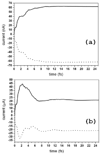
Figure 6: The solid (dotted) line represents the transient current through $S_{R}$ ($S_{L}$) driven by a step-like voltage $\Delta V^{R}(t)$ applied on the lead $R$ with the amplitude (a) $\Delta V^{R}=-1$ mV, and (b) $\Delta V^{R}=-1$ V.

In Fig. 6(a) and (b) we plot the transient currents through the interfaces $S_{L}$ and $S_{R}$, $J_{L}(t)$ and $J_{R}(t)$, for cases where the turn-on voltage $\Delta V^{R}=-1$ mV and $\Delta V^{R}=-1$ V, respectively. The EOM (19) is integrated numerically by the fourth-order Runge-Kutta method kutta up to $25$ fs with the time step $0.02$ fs. $J_{L}(t)$ and $J_{R}(t)$ depicted in Fig. 6(a) increase rapidly in the first $5$ fs and then approach gradually towards their steady state values. The steady currents through the leads $L$ and $R$ are $-62.8$ nA and $62.8$ nA, respectively, and thus cancel each other out exactly, as they should. With a much larger turn-on voltage $\Delta V^{R}$, $J_{L}(t)$ and $J_{R}(t)$ exhibit conspicuous overshooting during the first $2$ fs, as shown in Fig. 6(b), and afterwards they decay slowly to their steady state values, i.e., $-21.4$ $\mu$A and $21.4$ $\mu$A, respectively. From the both cases shown in Fig. 6 diversified fluctuations are observed for the time-dependent currents. This is due to the various eigenvalues possessed by the non-negative definite line-widths $\Lambda^{\alpha}$ with their magnitudes ranging from $0$ to $39$ eV, corresponding to various dissipative channels between $D$ and $L$ or $R$. For much higher turn-on voltages the linearized form for $\delta h^{XC}_{D}(t)$ (Eq. (24)) becomes inadequate, which makes such a TDDFT calculation computationally demanding with our present coding. From Fig. 6, the characteristic switch-on time for the model molecular device depicted in Fig. 5 is estimated as about $10$ fs for applied bias voltages as large as $1$ V.

VII Discussion and Summary

With an explicit form of the universal dissipation functional $Q_{\alpha}$, the time evolution of an open electron system in external fields is fully characterized by the EOM for the reduced single-electron density matrix of the reduced system (see Eq. (19)). In practical calculations, we need thus focus only on the reduced system with appropriate boundary conditions. In conventional quantum dissipation theory (QDT) qdt the key quantity is the reduced system density matrix. Whereas in Eq. (19) the basic variable is the reduced single-electron density matrix, which leads to the drastic reduction of the degrees of freedom in numerical simulation. Linear-scaling methods such as the localized-density-matrix method ldmtddft ; ldm may thus be adopted to further speed up the solution process of Eq. (19). Yokojima et al. developed a dynamic mean-field theory for dissipative interacting many-electron systems yokojima1 ; yokojima2 . An EOM for the reduced single-electron density matrix was derived to simulate the excitation and nonradiative relaxation of a molecule embedded in a thermal bath. This is in analogy to our case although our environment is actually a fermion bath instead of a boson bath. More importantly the number of electrons in the reduced system is conserved in Refs. yokojima1 ; yokojima2 while in our case it is not. Therefore, Eq. (19) provides a rigorous and convenient formalism to investigate the dynamic properties of open systems. Recently Cui et al. proposed a TDDFT scheme for first-principles study of non-equilibrium quantum transport based on the complete second-order quantum dissipation theory (CS-QDT) csqdt-scba , their formulation is constructed in terms of an improved reduced density matrix approach at the self-consistent Born approximation (SCBA) level.

It is worth mentioning that our first-principles method for open systems applies to the same phenomena, properties or systems as those intended by Hohenberg and Kohn hk , Kohn and Sham ks , and Runge and Gross tddft , i.e., where the exchange-correlation energy is a functional of electron density only, $E_{XC}=E_{XC}[\rho(\mathbf{r})]$. This is true when the interaction between the electric current and magnetic field is negligible. However, in the presence of a strong magnetic field, $E_{XC}=E_{XC}[\rho(\mathbf{r}),\mathbf{j}_{p}(\mathbf{r})]$ or $E_{XC}=E_{XC}[\rho(\mathbf{r}),\mathbf{B}(\mathbf{r})]$, where $\mathbf{j}_{p}(\mathbf{r})$ is the paramagnetic current density and $\mathbf{B}(\mathbf{r})$ is the magnetic field magdft . In such a case, our first-principles formalism needs to be generalized to include $\mathbf{j}_{p}(\mathbf{r})$ or $\mathbf{B}(\mathbf{r})$. Of course, $\mathbf{j}_{p}(\mathbf{r})$ or $\mathbf{B}(\mathbf{r})$ should be an analytical function in space. It is important to note that our formalism applies in principle to Cini’s scheme. Caroli’s scheme is employed to derive an approximated expression for the dissipative functional $Q_{\alpha}$.

To summarize, we have proved rigorously the existence of a first-principles method for time-dependent open electronic systems, and developed a formally closed TDDFT formalism by introducing a new dissipation functional. This new functional $Q_{\alpha}$ depends only on the electron density function of the reduced system. With an efficient WBL scheme for $Q_{\alpha}$, we have applied the first-principles formalism to carry out a TDDFT calculation for transient current through a model molecular device. This work greatly extends the realm of density-functional theory.

Appendix A Derivation of Eq. (7)

In Keldysh formalism keldysh , the nonequilibrium single-electron Green’s function $G_{k_{\alpha},m}(t,t^{\prime})$ is defined by

$$G_{k_{\alpha}m}(t,t^{\prime})=-i\left\langle T_{C}\!\left\{a_{k_{\alpha}}\!(t)\,a_{m}^{{\dagger}}(t^{\prime})\right\}\right\rangle,$$ (26)

where $T_{C}$ is the contour-ordering operator along the Keldysh contour keldysh . Its lesser component, $G^{<}_{k_{\alpha},m}(t,t^{\prime})$, is defined by

$$G^{<}_{k_{\alpha}m}(t,t^{\prime})=i\langle\,a^{{\dagger}}_{m}(t^{\prime})\,a_{k_{\alpha}}(t)\rangle.$$ (27)

Therefore $\sigma_{k_{\alpha}m}(t)$ is precisely the lesser Green’s function of identical time variables, i.e., $\sigma_{k_{\alpha}m}(t)=-iG^{<}_{k_{\alpha}m}(t,t^{\prime})|_{t^{\prime}=t}$. The formal NEGF theory has exactly the same structure as that of the time-ordered Green’s function at zero temperature. Thus, the Dyson equation for $G_{k_{\alpha}m}(t,t^{\prime})$ can be written as

$$G_{k_{\alpha}m}(t,t^{\prime})=\sum_{l\in D}\int_{C}d\tau\,g_{k_{\alpha}}(t,\tau)\,h_{k_{\alpha}l}(\tau)\,G_{lm}(\tau,t^{\prime}),$$ (28)

where $G_{lm}(\tau,t^{\prime})$ and $g_{k_{\alpha}}(t,\tau)$ are the contour-ordered Green’s functions for the reduced system $D$ and the isolated lead $\alpha$ ($L$ or $R$), respectively. Applying the analytic continuation rules of Langreth langreth , we have

$$G^{<}_{k_{\alpha}m}(t,t^{\prime}) = \sum_{l\in D}\int_{-\infty}^{\infty}d\tau\,h_{k_{\alpha}l}(\tau)\Big{[}g^{<}_{k_{\alpha}}(t,\tau)\,G^{a}_{lm}(\tau,t^{\prime})$$ (29)

$$+\,\,g^{r}_{k_{\alpha}}(t,\tau)\,G^{<}_{lm}(\tau,t^{\prime})\Big{]},$$

where $G^{a}_{lm}(\tau,t^{\prime})$ and $G^{<}_{lm}(\tau,t^{\prime})$ are the advanced and lesser Green’s functions for the reduced system $D$, respectively, and $g^{r}_{k_{\alpha}}(t,\tau)$ and $g^{<}_{k_{\alpha}}(t,\tau)$ are the retarded and lesser Green’s functions for the isolated lead $\alpha$ ($L$ or $R$) prb94win , respectively. Note that

$$G^{<}_{mk_{\alpha}}(t^{\prime},t)\! = i\langle a^{{\dagger}}_{k_{\alpha}}(t)\,a_{m}(t^{\prime})\rangle$$ (30)

$$= -\left[G^{<}_{k_{\alpha}m}(t,t^{\prime})\right]^{\ast}.$$

Obviously $\sigma_{mk_{\alpha}}(t)=-iG^{<}_{mk_{\alpha}}(t^{\prime},t)|_{t^{\prime}=t}$. Combining Eqs. (29) and (30), we obtain

$$G^{<}_{mk_{\alpha}}(t^{\prime},t) = \sum_{l\in D}\int_{-\infty}^{\infty}d\tau\,h_{lk_{\alpha}}(\tau)\Big{[}g^{<}_{k_{\alpha}}(\tau,t)\,G^{r}_{ml}(t^{\prime},\tau)+$$ (31)

$$g^{a}_{k_{\alpha}}(\tau,t)\,G^{<}_{ml}(t^{\prime},\tau)\Big{]}$$

by employing the following equalities:

$$G^{r}_{ml}(t^{\prime},\tau) = \left[G^{a}_{lm}(\tau,t^{\prime})\right]^{\ast},$$

$$G^{<}_{ml}(t^{\prime},\tau) = -\left[G^{<}_{lm}(\tau,t^{\prime})\right]^{\ast},$$

$$g^{a}_{k_{\alpha}}(\tau,t) = \left[g^{r}_{k_{\alpha}}(t,\tau)\right]^{\ast},$$

$$g^{<}_{k_{\alpha}}(\tau,t) = -\left[g^{<}_{k_{\alpha}}(t,\tau)\right]^{\ast}.$$ (32)

By inserting Eqs. (29) and (31) into Eq. (4), Eq. (7) is recovered straightforwardly where the self-energy terms are defined by

$$\Sigma^{a}_{\alpha,lm}(t,\tau) = \sum\limits_{k_{\alpha}\in\alpha}h_{lk_{\alpha}}(t)\,g^{a}_{k_{\alpha}}(t,\tau)\,h_{k_{\alpha}m}(\tau),$$

$$\Sigma^{<}_{\alpha,nl}(t,\tau) = \sum\limits_{k_{\alpha}\in\alpha}h_{nk_{\alpha}}(t)\,g^{<}_{k_{\alpha}}(t,\tau)\,h_{k_{\alpha}l}(\tau),$$

$$\Sigma^{r}_{\alpha,nl}(t,\tau) = \sum\limits_{k_{\alpha}\in\alpha}h_{nk_{\alpha}}(t)\,g^{r}_{k_{\alpha}}(t,\tau)\,h_{k_{\alpha}l}(\tau).$$ (33)

Appendix B Wide-band limit approximation for dissipation functional $\mathbf{Q}_{\mathbf{\alpha}}$

Within the WBL scheme, the retarded and advanced self-energies become local in time prb94win ,

$$\Sigma^{a}_{\alpha,nm}(\tau,t) = \sum_{k_{\alpha}\in\alpha}h_{nk_{\alpha}}(t)h_{k_{\alpha}m}(\tau)g^{a}_{k_{\alpha}}(\tau,t)$$ (34)

$$= \sum_{k_{\alpha}\in\alpha}h_{nk_{\alpha}}(t)h_{k_{\alpha}m}(\tau)$$

$$\times\,\left[\,i\vartheta(t-\tau)\,\mbox{e}^{\,i\epsilon_{k}^{\alpha}(t-\tau)}\,\mbox{e}^{\,i\int^{t}_{\tau}\Delta\epsilon^{\alpha}(\bar{t})\,d\bar{t}}\,\right]$$

$$= \frac{i}{\pi}\,\vartheta(t-\tau)\,\mbox{e}^{\,i\int^{t}_{\tau}\Delta\epsilon^{\alpha}(\bar{t})\,d\bar{t}}$$

$$\times\left\{\int_{-\infty}^{+\infty}\mbox{e}^{i\epsilon(t-\tau)}d\epsilon\right\}\Lambda^{\alpha}_{nm}$$

$$= i\delta(t-\tau)\Lambda^{\alpha}_{nm},$$

$$\Sigma^{r}_{\alpha,nm}(\tau,t) = \left[\Sigma^{a}_{\alpha,mn}(t,\tau)\right]^{\ast}$$ (35)

$$= -i\delta(t-\tau)\Lambda^{\alpha}_{nm}.$$

The third equality of Eq. (34) involves the following approximation for the line-widths within the WBL scheme,

$$\Lambda^{\alpha}_{k}(t,\tau) \equiv \pi\,\eta_{\alpha}(\epsilon^{\alpha}_{k})\,h_{nk_{\alpha}}(t)\,h_{k_{\alpha}m}(\tau)$$ (36)

$$\approx \Lambda^{\alpha}(t,\tau)\approx\Lambda^{\alpha}.$$

Initially the entire system ($D$ + $L$ + $R$) is in its ground state with the chemical potential $\mu^{0}$, from the time $t=0$ it is switched on by external potentials $\Delta V^{\alpha}(t)$ applied on the leads $L$ or $R$. Hence, for $t,\tau>0$ we have

$$\Sigma^{<}_{\alpha,nm}(\tau,t) = \sum_{k_{\alpha}\in\alpha}h_{nk_{\alpha}}(t)h_{k_{\alpha}m}(\tau)g^{<}_{k_{\alpha}}(\tau,t)$$ (37)

$$= \sum_{k_{\alpha}\in\alpha}h_{nk_{\alpha}}(t)h_{k_{\alpha}m}(\tau)$$

$$\times\left[i\,f^{\alpha}(\epsilon^{\alpha}_{k})\,\mbox{e}^{\,i\epsilon_{k}^{\alpha}(t-\tau)}\,\mbox{e}^{\,i\int^{t}_{\tau}\Delta\epsilon^{\alpha}(\bar{t})\,d\bar{t}}\,\right]$$

$$= \frac{2i}{\pi}\,\mbox{e}^{\,i\int^{t}_{\tau}\Delta\epsilon^{\alpha}(\bar{t})\,d\bar{t}}\,\Lambda^{\alpha}_{nm}$$

$$\times\left\{\int_{-\infty}^{+\infty}f^{\alpha}(\epsilon)\,\mbox{e}^{\,i\epsilon(t-\tau)}d\epsilon\right\},$$

$$G^{r}_{nm}(t,\tau) = -i\vartheta(t-\tau)\sum_{l\in D}U^{(-)}_{nl}(t)U^{(+)}_{lm}(\tau),$$ (38)

where $\Delta\epsilon^{\alpha}(t)=-\Delta V^{\alpha}(t)$ are the time-dependent level shifts for the leads $L$ and $R$, while for $\tau<0$ and $t>0$, the counterparts of (37) and (38) are as the following:

$$\Sigma^{<}_{\alpha,nm}(\tau,t) = \sum_{k_{\alpha}\in\alpha}h_{nk_{\alpha}}(t)h_{k_{\alpha}m}(\tau)\,g^{<}_{k_{\alpha}}(\tau,t)$$ (39)

$$= \sum_{k_{\alpha}\in\alpha}h_{nk_{\alpha}}(t)h_{k_{\alpha}m}(\tau)$$

$$\times\,\Big{[}i\,f^{\alpha}(\epsilon^{\alpha}_{k})\,\mbox{e}^{\,i\epsilon^{\alpha}_{k}(t-\tau)}\mbox{e}^{\,i\int^{t}_{0}\Delta\epsilon^{\alpha}(\bar{t})\,d\bar{t}}\,\Big{]}$$

$$= \frac{2i}{\pi}\,\mbox{e}^{\,i\int^{t}_{0}\Delta\epsilon^{\alpha}(\bar{t})\,d\bar{t}}\,\Lambda^{\alpha}_{nm}$$

$$\times\,\left\{\int_{-\infty}^{+\infty}f^{\alpha}(\epsilon)\,\mbox{e}^{\,i\epsilon(t-\tau)}d\epsilon\right\},$$

$$G^{r}_{nm}(t,\tau) = \sum_{l\in D}U^{(-)}_{nl}(t)\,G^{r}_{lm}(0,\tau)$$ (40)

$$= \sum_{l\in D}U^{(-)}_{nl}(t)\,G^{r,\,0}_{lm}(-\tau),$$

where $G^{r,\,0}_{lm}(-\tau)$ is the retarded Green’s function for the reduced system $D$ before switch-on. The propagators for the reduced system $U^{(\pm)}(t)$ are defined as

$$U^{(\pm)}(t) = \exp\bigg{\{}\pm i\int_{0}^{t}\!h_{D}(\tau)d\tau\pm\Lambda\,t\bigg{\}}.$$ (41)

where $\Lambda=\sum_{\alpha=L,R}\Lambda^{\alpha}$. By inserting Eqs. (34)$-$(40) into Eq. (7) the explicit form of WBL approximation for the dissipation functional $Q_{\alpha}$ is obtained as

$$Q^{WBL}_{\alpha}(t) = K^{\alpha}(t)+\left\{\Lambda^{\alpha},\sigma_{D}(t)\right\},$$ (42)

where the curly bracket on the RHS denotes an anticommutator, and $K^{\alpha}(t)$ is a Hermitian matrix expressed by

$$K^{\alpha}(t) = P^{\alpha}(t)+\left[P^{\alpha}(t)\right]^{\dagger},$$ (43)

where $P^{\alpha}(t)$ involve an integration over the entire $t$-space, which is then decomposed into positive and negative parts, denoted by $P^{(+)}_{\alpha}(t)$ and $P^{(-)}_{\alpha}(t)$, respectively.

$$P^{\alpha}(t) = -\int_{-\infty}^{+\infty}d\tau\,G^{r}_{D}(t,\tau)\Sigma^{<}_{\alpha}(\tau,t)$$ (44)

$$= P_{\alpha}^{(-)}(t)+P_{\alpha}^{(+)}(t).$$

$P_{\alpha}^{(-)}(t)$ and $P_{\alpha}^{(+)}(t)$ are evaluated via

$$P_{\alpha}^{(-)}(t) = -\int_{-\infty}^{0}d\tau\,G^{r}_{D}(t,\tau)\Sigma^{<}_{\alpha}(\tau,t)$$ (45)

$$= -\frac{2i}{\pi}\,\,\mbox{exp}\left\{i\!\int_{0}^{t}\Delta\epsilon^{\alpha}\!(\tau)d\tau\right\}U^{(-)}(t)$$

$$\times\left\{\int_{-\infty}^{\mu^{0}}\frac{d\epsilon\,\mbox{e}^{i\epsilon t}}{\epsilon-h_{D}(0)+i\,\Lambda}\right\}\Lambda^{\alpha},$$

and

$$P_{\alpha}^{(+)}(t) = -\frac{2}{\pi}\int^{\mu^{0}}_{-\infty}d\epsilon\,W_{\alpha}^{(-)}(\epsilon,t)$$ (46)

$$\times\int^{t}_{0}d\tau\,W_{\alpha}^{(+)}(\epsilon,\tau)\,\Lambda^{\alpha},$$

respectively, where

$$W_{\alpha}^{\pm}(\epsilon,t) = \mbox{e}^{\pm\,i\int^{t}_{0}d\tau\left[h_{D}(\tau)-i\Lambda-\Delta\epsilon^{\alpha}(\tau)-\epsilon\right]}.$$ (47)

However, the evaluations of Eqs. (46)-(47) are found extremely time-consuming since at every time $t$ one needs to propagate $W_{\alpha}^{\pm}(\epsilon,t)$ for every individual $\epsilon$ inside the lead energy spectrum. It is thus necessary to seek for a simpler approximate form for $P^{(+)}_{\alpha}(t)$ with satisfactory accuracy retained. Note that Eq. (46) can be reformulated as

$$P_{\alpha}^{(+)}(t) = -\frac{2}{\pi}\int_{-\infty}^{\mu^{0}}d\epsilon\int_{0}^{t}d\tau$$ (48)

$$\times\,\mbox{e}^{-i\int_{\tau}^{t}\left[h_{D}(\bar{t})-i\Lambda-\Delta\epsilon^{\alpha}(\bar{t})-\epsilon\right]d\bar{t}}\,\Lambda^{\alpha}.$$

For cases where a steady state can be ultimately reached, $\Delta\epsilon^{\alpha}(t)$ and $h_{D}(t)$ become asymptotically constant as time $t\rightarrow+\infty$, i.e., $\Delta\epsilon^{\alpha}(t)\rightarrow\Delta\epsilon^{\alpha}(\infty)$ and $h_{D}(t)\rightarrow h_{D}(\infty)$. Therefore, the steady state $P_{\alpha}^{(+)}(\infty)$ can be approximated by substituting $\Delta\epsilon^{\alpha}(\infty)$ and $h_{D}(\infty)$ for $\Delta\epsilon^{\alpha}(t)$ and $h_{D}(t)$ in Eq. (48), respectively.

$$P_{\alpha}^{(+)}(\infty) \approx -\frac{2}{\pi}\int_{-\infty}^{\mu^{0}}d\epsilon\int_{0}^{t}d\tau\$$ (49)

$$\times\,\mbox{e}^{-i\left[h_{D}(\infty)-i\Lambda-\Delta\epsilon^{\alpha}(\infty)-\epsilon\right](t-\tau)}\,\Lambda^{\alpha}$$

$$= -\frac{2i}{\pi}\int_{-\infty}^{\mu^{0}}\left\{I-\mbox{e}^{-i\left[h_{D}(\infty)-i\Lambda-\Delta\epsilon^{\alpha}(\infty)-\epsilon\right]t}\right\}$$

$$\times\,\frac{d\epsilon}{\epsilon-h_{D}(\infty)+i\Lambda+\Delta\epsilon^{\alpha}(\infty)}\,\Lambda^{\alpha}.$$

It is obvious from Eq. (48) that

$$P_{\alpha}^{(+)}(0)=0.$$ (50)

Thus $P_{\alpha}^{(+)}(t)$ for any time $t$ between $0$ and $+\infty$ can be approximately expressed by adiabatically connecting Eq. (49) with (50) as follows,

$$P_{\alpha}^{(+)}(t) \approx -\frac{2i}{\pi}\int_{-\infty}^{\mu^{0}}\left\{I-\mbox{e}^{-i\int_{0}^{t}\left[h_{D}(\tau)-i\Lambda-\Delta\epsilon^{\alpha}(\tau)-\epsilon\right]d\tau}\right\}$$ (51)

$$\times\,\frac{d\epsilon}{\epsilon-h_{D}(t)+i\Lambda+\Delta\epsilon^{\alpha}(t)}\,\Lambda^{\alpha}.$$

Both Eqs. (48) and (51) lead to the correct $P^{\alpha}(\infty)$ for steady states,

$$P^{\alpha}(\infty) = -\frac{2i}{\pi}\!\int_{-\infty}^{\mu^{0}}\!d\epsilon$$ (52)

$$\times\,\frac{1}{\epsilon-h_{D}(\infty)+i\Lambda+\Delta\epsilon^{\alpha}(\infty)}\,\Lambda^{\alpha},$$

If the external applied voltage assumes a step-like form, for instance, $\Delta V^{\alpha}(t)=-\Delta\epsilon^{\alpha}(t)=\Delta V^{\alpha}(1-\mbox{e}^{-t/a})$ with $a\rightarrow 0^{+}$, and $h_{D}(t)$ is not affected by the fluctuation of $\sigma_{D}(t)$, Eq. (51) would recover exactly Eq. (48). In other cases, Eq. (51) provides an accurate and efficient approximation for Eq. (48), so long as $\Delta V^{\alpha}(t)$ do not vary dramatically in time. Since the integration over energy in Eq. (51) can be performed readily by transforming the integrand into diagonal representation, Eq. (51) is evaluated much faster than Eq. (48). Due to its efficiency and accuracy, Eq. (51) is combined with Eqs. (42)-(45) to form the WBL approximation for the dissipation functional $Q^{WBL}_{\alpha}$, and thus recovers Eq. (21) of Sec. V.

As discussed in Sec. V, $Q^{WBL}_{\alpha}(t)$ depends explicitly on $\Delta V^{\alpha}(t)$, $\sigma_{D}(t)$, $h_{D}(t)$ and $\Lambda^{\alpha}$, where $h_{D}(t)$ is directly related to $\rho_{D}(\mathbf{r},t)$ by the Poisson equation on $D$ subjected to boundary conditions $\Delta V^{\alpha}(t)$, and $\Lambda^{\alpha}$ are associated with the DOS of $D$ near the surfaces $S_{\alpha}$. Therefore in practice $Q^{WBL}_{\alpha}$ is a functional of $\rho_{D}(\mathbf{r},t)$ only, i.e.,

$$Q^{WBL}_{\alpha}(t) \equiv Q^{WBL}_{\alpha}\Big{[}\sigma_{D}\!\left[\rho_{D}\right],\,h_{D}[\sigma_{D}\!\left[\rho_{D}\right],t],$$ (53)

$$\Lambda^{\alpha}[\rho_{D},t],\,\Delta V^{\alpha}[\rho_{D},t],\,t\Big{]}.$$

References

- (1)
- (2) P. Hohenberg and W. Kohn, Phys. Rev. 136, B 864, (1964)
- (3) W. Kohn and L. J. Sham, Phys. Rev. 140, A 1133 (1965)
- (4) E. Runge and E. K. U. Gross, Phys. Rev. Lett. 52, 997 (1984)
- (5) N. D. Lang and Ph. Avouris, Phys. Rev. Lett. 84, 358 (2000)
- (6) J. Heurich, J. C. Cuevas, W. Wenzel and G. Schön, Phys. Rev. Lett. 88, 256803 (2002)
- (7) C.-K. Wang and Y. Luo, J. Chem. Phys. 119, 4923 (2003)
- (8) N. D. Lang, Phys. Rev. B 52, 5335 (1995)
- (9) Y. Xue, S. Datta and M. A. Ratner, J. Chem. Phys. 115, 4292 (2001)
- (10) J. Taylor, H. Guo and J. Wang, Phys. Rev. B. 63, 245407 (2001)
- (11) S.-H. Ke, H. U. Baranger and W. Yang, J. Am. Chem. Soc. 126, 15897 (2004)
- (12) W.-Q. Deng, R. P. Muller and W. A. Goddard III, J. Am. Chem. Soc. 126, 13563 (2004)
- (13) M. Brandbyge et al., Phys. Rev. B 65, 165401 (2002)
- (14) Y. Xue, S. Datta and M. A. Ratner, Chem. Phys. 281, 151 (2002)
- (15) D. S. Kosov, J. Chem. Phys. 119, 1 (2003)
- (16) K. Burke, R. Car and R. Gebauer, Phys. Rev. Lett. 94, 146803 (2005)
- (17) C. Y. Yam, S. Yokojima and G.H. Chen, J. Chem. Phys. 119, 8794 (2003); Phys. Rev. B 68, 153105 (2003)
- (18) M. E. Casida, Recent Developments and Applications in Density Functional Theory, Elsevier, Amsterdam (1996)
- (19) L. V. Keldysh, JETP 20, 1018 (1965)
- (20) D. C. Langreth and P. Nordlander, Phys. Rev. B 43, 2541 (1991)
- (21) A.-P. Jauho, N. S. Wingreen and Y. Meir, Phys. Rev. B 50, 5528 (1994)
- (22) G. Stefanucci and C.-O. Almbladh, Europhys. Lett. 67 (1), 14 (2004)
- (23) M. Cini, Phys. Rev. B 22, 5887 (1980)
- (24) C. Caroli, R. Combescot, P. Nozìeres and D. Saint-James, J. Phys. C 4, 916 (1971); C. Caroli, R. Combescot, D. Lederer, P. Nozìeres and D. Saint-James, J. Phys. C 4, 2598 (1971)
- (25) S. Datta, Electronic Transport in Mesoscopic Systems, Cambridge University Press (1995)
- (26) R. Landauer, Philos. Mag. 21, 863 (1970)
- (27) X. Zheng and G.H. Chen, arXiv:physics/0502021 (2005)
- (28) J. Riess and W. Münch, Theoret. Chim. Acta 58, 295 (1981)
- (29) P. G. Mezey, Mol. Phys. 96, 169 (1999)
- (30) S. Fournais, M. Hoffmann-Ostenhof and T. Hoffmann-Ostenhof, Commun. Math. Phys. 228, 401 (2002); S. Fournais, M. Hoffmann-Ostenhof, T. Hoffmann-Ostenhof and T. Ø. Sørensen, Ark. Mat. 42, 87 (2004)
- (31) T. A. Wesolowski and A. Warshel, J. Phys. Chem. 97, 8050 (1993)
- (32) J. Maciejko, J. Wang and H. Guo, cond-mat/0603254 (2006).
- (33) M. P. López Sancho, J. M. López Sancho and J. Rubio, J. Phys. F: Met. Phys. 15, 851 (1985)
- (34) W. H. Press, B. P. Flannery, S. A. Teukolsky and W. T. Vetterling, Numerical Recipes in C, Cambridge University Press (1988)
- (35) Y. Yan, Phys. Rev. A 58, 2721 (1998); R. Xu and Y. Yan, J. Chem. Phys. 116 9196 (2002)
- (36) S. Yokojima and G.H. Chen, Chem. Phys. Lett. 292, 379 (1998); Phys. Rev. B 59, 7259 (1999).
- (37) S. Yokojima and G.H. Chen, Chem. Phys. Lett. 355, 400 (2002)
- (38) S. Yokojima, G.H. Chen, R. Xu and Y. Yan, Chem. Phys. Lett. 369, 495 (2003); J. Comp. Chem. 24, 2083 (2003)
- (39) Ping Cui, Xin-Qi Li, Jiushu Shao and Yijing Yan, cond-mat/0506477 (2005)
- (40) G. Vignale and M. Rasolt, Phys. Rev. Lett. 59, 2360 (1987); C. J. Grayce and R. A. Harris, Phys. Rev. A 50, 3089 (1994)