Interpreting concurrence in terms of covariances in a generalized spin star system

Abstract

The quantum dynamics of $M$ pairwise coupled spin $\frac{1}{2}$ is analyzed and the time evolution of the entanglement get established within a prefixed couple of spins is studied. A conceptual and quantitative link between the concurrence function and measurable quantities is brought to light providing a physical interpretation for the concurrence itself as well as a way to measure it. A generalized spin star system is exactly investigated showing that the entanglement accompanying its rich dynamics is traceable back to the covariance of appropriate commuting observables of the two spins.

I Introduction

Quite recently a growing attention has been devoted to interacting spin systems Loss ; Karbach ; Dobrovitski ; Geza ; Cucchietti also in view of the fact that they can be successfully used for gate operations in solid state quantum computation processors Karbach ; Burkard ; Awschalom ; Imamoglu . They indeed provide scalable systems that can be easily integrated into standard silicon technology. Spin sets with an assigned one- or multi-dimensional spatial distribution appear to be comparatively more promising candidates for the realization of entangled states in matter systems.

Numerous papers published over the last few years witness the central role played by spin systems, both from a theoretical and applicative point of view, in the emerging field of quantum entanglement in solid state physics. As an example, and in connection to the subject we are going to discuss in the present paper, it is worth explicitly citing those papers dealing with investigation on the entanglement get established within a pair of spins belonging to a spin ensemble whose dynamics is dominated by XXX XXX , XXZ XXZ , XYZ XYZ1 ; XYZ2 and XY XY1 ; XY2 Heisenberg interaction models. In these cases the analysis is developed through the evaluation of the concurrence function appropriate to estimate the degree of quantum correlations get established in a two-spin system.

It is important to underline that generally speaking quantifying and controlling entanglement is a crucial challenge both from a theoretical point of view and in consideration of its applicative potentialities in various field of quantum information. It is in addition important to stress that studying spin systems is however of remarkable interest in its own. It is well known, for example, that a magnetic sample can be suitably analyzed adopting a general Hamiltonian model describing a system of $N$ spins coupled by exchange interactions with arbitrary range and strength magnetism .

In this paper we study the quantum dynamics of a system of $M$ Heisenberg pairwise coupled spins $\frac{1}{2}$ investigating in particular the time evolution of the entanglement get established within a spin pair subsystem. The analysis here reported enable us to bring to light a new conceptual and quantitative link between the concurrence function and an observable quantity having a clear physical meaning suggesting, at the same time, a simple way of measuring entanglement in a two spin system without necessarily reconstructing its state. Our approach focusses on a generalized spin star system whose dynamics provides an enlightening key to go deep into the physical meaning of entanglement and concurrence. In this framework we succeed in giving a simple recipe to control the ability of the system in developing only classical or also quantum correlations.

II Heisenberg Interacting spin systems

Our physical system consists of $M$ two-level objects whose quantum dynamics is completely described by spin operators $\vec{S}^{(i)}\equiv 2\vec{\sigma}^{(i)}$ $(i=1,...,M)$, $\vec{\sigma}^{(i)}$ being the Pauli matrix operator pertaining to the $i-$th two-level subsystem. The cartesian components of $\vec{S}^{(i)}$, $S_{x}^{(i)},S_{y}^{(i)}$, and $S_{z}^{(i)}$, fulfill the usual angular momentum commutation relations and $|\pm 1_{i}\rangle$ denote the two eigenstates of $\sigma_{z}^{(i)}$ that is $\sigma_{z}^{(i)}|\pm 1_{i}\rangle=\pm|\pm 1_{i}\rangle$.

In this section we wish to keep our presentation general enough to encompass several possible physical scenarios of interest. Thus we adopt the assumption that a spin pair $(i,j)$ belonging to our ensemble of $M$ spins $(i,j=1,2,...,M;\;i\neq j)$ experiences an Heisenberg exchange-like interaction describable as proportional to $\vec{S}^{(i)}\cdot\vec{S}^{(i)}$. The hamiltonian model representing such a physical situation in the interaction picture with respect to the free hamiltonian

$$H_{0}=\omega\sum_{i=1}^{M}S_{z}^{(i)}$$ (1)

may be cast in the following general form

$$H_{I}=\sum_{j>i=1}^{M}{\alpha_{ij}\vec{S}^{(i)}\cdot\vec{S}^{(j)}}$$ (2)

$\alpha_{ij}$ being a real coupling constant left undetermined at the moment. Since $H_{I}$ is a scalar operator with respect to $\vec{S}=\sum_{i}\vec{S}^{(i)}$ and in addition commutes with $H_{0}$, then the $z-$component of $\vec{S}$ as well as $S^{2}$ are constants of motion. As a consequence, preparing the $M$ spins in an eigenstate of $S_{z}$, the total system evolves in the correspondent invariant Hilbert subspace. It is not difficult to convince oneself that the reduced density matrix relative to a prefixed couple of spins, say the spins $i$ and $j$, when expressed into the standard two-spin basis

$$\{|1_{i},1_{j}\rangle,|1_{i},-1_{j}\rangle,|-1_{i},1_{j}\rangle,|-1_{i},-1_{j}\rangle\}$$ (3)

assumes a block diagonal form, each block being biunivocally singled out by one of the three possible eigenvalues of $S_{z}^{(ij)}$$\equiv(S_{z}^{(i)}+S_{z}^{(j)})$. Stated another way, the reduced density matrix $\rho_{ij}(t)$, obtained tracing the density operator of the closed system over the degrees of freedom relative to all the $M$ spins except $i$ and $j$, assumes the quite simple form

$$\rho_{ij}(t)=\left(\begin{array}[]{cccc}a(t)&0&0&0\\ 0&b(t)&c(t)&0\\ 0&c^{*}(t)&d(t)&0\\ 0&0&0&e(t)\end{array}\right)$$ (4)

when represented in the ordered basis given by eq. (3) Pratt . We wish to stress that the possibility of writing $\rho_{ij}(t)$ as in eq. (4) directly stems from the initial preparation being instead independent on the values of the coupling constants set $\{\alpha_{ij}\}$. On the contrary, the matrix elements of $\rho_{ij}$ depend on this set too.

Scope of this section is to prove the existence of dynamical properties of our system of $M$ spins relying solely on the structure of the density matrix $\rho_{ij}(t)$ and not on the specific form of the functions $a(t)$, $b(t)$,…, $e(t)$ appearing in eq. (4).

This circumstance appears still more remarkable at the light of the fact that, generally speaking, it is not possible to exactly solve the dynamics of $M$ interacting spins described by the hamiltonian model (2). Thus results obtained just exploiting the form of the two-spin reduced density operator $\rho_{ij}(t)$ (4), besides being valid whatever the coupling constants are, also provide peculiar tools to test approximate dynamical solutions when we are unable to exactly solve the system dynamics.

With these considerations in mind, we now focus on a system of two spins $\frac{1}{2}$ described at a generic time instant $t$ by a density matrix like (4) without specifying the analytic expression of the four population functions $a(t)$, $b(t)$,$d(t)$, $e(t)$ and the coherence function $c(t)$.

Let’s begin by observing that in order to guarantee that the operator given by equation (4) represents indeed a density matrix, the inequality

$$|c(t)|\leq\sqrt{b(t)d(t)}$$ (5)

must be satisfied at any time instant $t$ Landau . It is easy to demonstrate that this relation directly stems from the requirement that all the eigenvalues of $\rho_{ij}$ are not negative.

An interesting property assumed by each density matrix belonging to the class defined by eq. (4) concerns the possibility of getting a bridge between the Peres-Horodecki (P-H) separability condition P-H1 ; P-H2 and the measure of entanglement proposed by Wootters Wootters98 . The P-H separability criterium claims that the density matrix $\rho$ of a bipartite system composed by two-level subsystems, is separable if and only if all the eigenvalues of the matrix $\sigma$ obtained from $\rho$ transposing with respect to the indices of only one subsystem, are not negative. In our case such a matrix, built up from $\rho_{ij}$, may be cast as follows

$$\sigma_{ij}(t)=\left(\begin{array}[]{cccc}a(t)&0&0&c^{*}(t)\\ 0&b(t)&0&0\\ 0&0&d(t)&0\\ c(t)&0&0&e(t)\end{array}\right)$$ (6)

Thus applying the P-H separability criterium, it is easy to demonstrate that our two-spin density matrix (4) is separable at a fixed time instant $t$ if and only if the condition

$$|c(t)|\leq\sqrt{a(t)e(t)}$$ (7)

is fulfilled. On the other hand, when the density operator of two two-level systems has the simple form of eq. (4) it is quite straightforward to evaluate the concurrence function $C_{onc}(t)$, introduced by Wootters as a measure of entanglement in bipartite system composed by two qubits, getting

$$C_{onc}(t)=Max\{0,2(|c(t)|-\sqrt{a(t)e(t)})\}$$ (8)

Considering eq. (8) we immediately deduce that at a generic time instant $t$ the system is characterized by absence of entanglement if and only if condition (7) is satisfied in accordance with the P-H separability criterium.

Let’s in addition remark that the presence of entanglement at a time instant $t$ necessarily implies the existence of at least a couple of operators $A^{(i)}$ and $B^{(j)}$ acting on the bidimensional Hilbert spaces of the spin $i$ and $j$ respectively, such that the correlation function

$$C_{AB}(t)\equiv Tr\{\rho_{ij}(t)A^{(i)}B^{(j)}\}$$

$$-Tr_{i}\{\rho_{i}(t)A^{(i)}\}Tr_{j}\{\rho_{j}(t)B^{(j)}\}$$ (9)

is different from zero. In eq. (II) $\rho_{k}$ $(k=i,j)$ is the reduced density matrix of the spin $k$ and $Tr_{k}$ denotes the trace with respect to its degrees of freedom. At the light of the results expressed by eq. (7) and (8) a suitable pair of operators satisfying eq. (II) must at least fulfill the condition of not being diagonal in the standard basis (3). Thus we are lead to consider the two operators $\sigma_{x}^{(i)}$ and $\sigma_{x}^{(j)}$. Exploiting the form of $\rho_{ij}(t)$ as given by eq. (4) it is immediate to demonstrate that

$$C_{\sigma_{x}\sigma_{x}}(t)=2\Re{[c(t)]}$$ (10)

since

$$\langle\sigma_{x}^{(k)}\rangle\equiv Tr_{k}\{\rho_{k}(t)\sigma_{x}^{(k)}\}=0\;\;\;\;(k=i,j)$$ (11)

and

$$\langle\sigma_{x}^{(i)}\sigma_{x}^{(j)}\rangle\equiv Tr\{\rho_{ij}(t)\sigma_{x}^{(i)}\sigma_{x}^{(j)}\}=2\Re{[c(t)]}$$ (12)

If instead we analogously consider the two operators $\sigma_{y}^{(i)}$ and $\sigma_{y}^{(j)}$ we obtain

$$C_{\sigma_{y}\sigma_{y}}(t)=2\Im{[c(t)]}$$ (13)

A comparison among eqs. (10), (13) and (8) brings to light the existence of a new direct link between the concurrence function and measurable quantities of clear physical meaning. We may indeed claim that when different from zero the concurrence function may be expressed as

$$C_{onc}(t)=\sqrt{C_{\sigma_{x}\sigma_{x}}^{2}+C_{\sigma_{y}\sigma_{y}}^{2}}-2\sqrt{a(t)e(t)}$$ (14)

$a(t)$ and $e(t)$ being the probability of finding both the spins $i$ and $j$ in their up states or down states respectively. It is in addition rather remarkable the fact that if $a(t)=0$ and/or $e(t)=0$ the concurrence as expressed by eq. (8) reduces to

$$C_{onc}(t)=2\sqrt{\Re{[c(t)]}^{2}+\Im{[c(t)]}^{2}}\equiv\sqrt{C_{\sigma_{x}\sigma_{x}}^{2}+C_{\sigma_{y}\sigma_{y}}^{2}}$$ (15)

so that it is zero only if both the two quantum covariances $C_{\sigma_{x}\sigma_{x}}(t)$ and $C_{\sigma_{y}\sigma_{y}}(t)$ vanish.

This elegant formula suggests in a very transparent way that the covariances between the $x$ and $y$ components of the two spins are suitable quantities in order to highlight the presence of entanglement in our two-spin system. It is however important to emphasize that $C_{\sigma_{x}\sigma_{x}}\neq 0$ $(C_{\sigma_{y}\sigma_{y}}\neq 0)$ doesn’t necessarily imply in its own that the system has developed quantum correlations. This aspect will appear more clear in the next section where we will analyze the exact dynamics of a specific system whose hamiltonian model is a particular case of that expressed by equation (2). Concluding this section we wish to stress that the quite simple form of $\rho_{ij}(t)$, given by eq. (4), which represents the starting point of our analysis, naturally arises in many physical contexts not necessarily involving spin $\frac{1}{2}$ systems. In particular the conditions under which eq. (15) has been derived are verified for example when the dynamics of two isolated atoms, each in its own Jaynes-Cummings cavity is studied cavity1 ; cavity2 ; cavity3 . In this sense, we may claim that the concepts and tools reported in this paper are flexible enough to be exported into physical situations more general than the spin system here envisaged.

III Generalized spin star system

Appropriately choosing the coupling constants $\alpha_{ij}$ the quite general hamiltonian model (2) can describe very different physical scenarios. Here we wish to focus on the case of a system composed by a pair of not directly interacting spins each one coupled to every two-level component of a set of $N$ spins by a physical mechanism representable by a XY Heisenberg exchange like term. If we stipulate the absence of any internal coupling within the set of $N$ spins, hereafter referred to as the spin bath, and indicate by $A$ and $B$ the two spins of the preferred couple, also called the central system, the hamiltonian model (2) assumes the following form

$$H_{XY}= \alpha_{A}(S_{x}^{A}\sum_{i=1}^{N}S_{x}^{i}+S_{y}^{A}\sum_{i=1}^{N}S_{y}^{i})+$$ (16)

$$+\alpha_{B}(S_{x}^{B}\sum_{i=1}^{N}S_{x}^{i}+S_{y}^{B}\sum_{i=1}^{N}S_{y}^{i})$$

It is worth noticing that specializing the hamiltonian model given by eq. (2) into the one expressed by eq. (16) we are supposing that the spin $A$ and $B$ couples with any element of the bath with a site-independent coupling constant $\alpha_{A}$ or $\alpha_{B}$ respectively.

The interest toward this system, representing a generalization of those systems reported in literature as spin star systems XY1 ; spinstar , arises from several considerations. First of all, as we are going to show, it is exactly solvable so that in this case we can explicitly know the functions $a(t)$, $b(t)$,…, $e(t)$ appearing in the density matrix given by eq. (4). This circumstance allows us to explore conditions for the emergence of and to investigate on the time evolution of correlations get established within the pair $A$ and $B$. A specific aspect of this study is in particular, the possibility of controlling the rising of only classical or also quantum correlations between the two not directly interacting spins in the central subsystem. Another important point worth to be emphasized is the fact that under appropriate initial conditions, the concurrence appearing and evolving within the $A-B$ subsystem may be traced back and interpreted in terms of simple measurable quantities. As a consequence we are in condition to suggest a way to measure the concurrence in laboratory without being obliged to reconstruct, as usually required, the state of the system.

Let’s begin by observing that the possibility of exactly solving the dynamics of the system described by (16), is strictly related to the existence of other constants of motion with respect to the general model (2).

Introducing the bath collective operators

$$\overrightarrow{J}=\sum_{i=1}^{N}\overrightarrow{S}^{(i)}$$ (17)

and

$$J_{\pm}=J_{x}\pm iJ_{y}$$ (18)

and casting the interaction hamiltonian (16) in the form

$$H_{XY}=\alpha_{A}(S_{+}^{A}J_{-}+S_{-}^{A}J_{+})+\alpha_{B}(S_{+}^{B}J_{-}+S_{-}^{B}J_{+})$$ (19)

it is indeed easy to convince oneself that

$$[H_{XY},J^{2}]=0$$ (20)

$$[H_{XY},J_{int}^{2}]=0$$ (21)

$\overrightarrow{J}_{int}$ being an intermediate angular momentum resulting from the coupling of selected at will individual angular momenta of the bath. For example defining $\overrightarrow{J}_{i,j}=\overrightarrow{S}^{(i)}+\overrightarrow{S}^{(j)}$, or $\overrightarrow{J}_{i,j,k}=\overrightarrow{J}_{i,j}+\overrightarrow{S}^{(k)}$, we deduce

$$[H_{XY},J_{i,j}^{2}]=0\;\;\;\;\;[H_{XY},J_{i,j,k}^{2}]=0$$ (22)

In order to make more evident how the existence of all these constants of motion provides the possibility of exactly solving the dynamics of the closed system constituted by the central one $(A,B)$ and the spin bath, let’s denote by $\{|J,M,\nu\rangle\}$ a bath coupled basis satisfying

$$J^{2}|J,M,\nu\rangle=J(J+1)|J,M,\nu\rangle$$ (23)

$$J_{z}|J,M,\nu\rangle=M|J,M,\nu\rangle$$ (24)

$\nu$ being an integer index taking into account the degeneracy with respect to the quantum numbers $J$ and $M$. As far as the ordered basis of the $(A,B)$ subsystem given by eq. (3), we introduce the new more compact notation $\{|\sigma_{z}^{A}(n),\sigma_{z}^{B}(n)\rangle,\;\;n=1,..,4\}$ putting

$$|\sigma_{z}^{A}(1),\sigma_{z}^{B}(1)\rangle\equiv|1_{A},1_{B}\rangle,$$

$$|\sigma_{z}^{A}(2),\sigma_{z}^{B}(2)\rangle\equiv|1_{A},-1_{B}\rangle,$$

$$|\sigma_{z}^{A}(3),\sigma_{z}^{B}(3)\rangle\equiv|-1_{A},1_{B}\rangle,$$

$$|\sigma_{z}^{A}(4),\sigma_{z}^{B}(4)\rangle\equiv|-1_{A},-1_{B}\rangle,$$ (25)

We can thus denote by $|J,M,\nu\rangle|\sigma_{z}^{A}(n),\sigma_{z}^{B}(n)\rangle$$\equiv|J,M,\nu,\sigma_{z}^{A}(n),\sigma_{z}^{B}(n)\rangle$ a generic state of the basis of the Hilbert space of the total system obtained as tensorial product of the two bases previously introduced.

It is immediate to convince oneself that the dynamical constraints imposed by the constants of motion put into evidence at the beginning of this section, allow us to claim that, starting from a state $|\sigma_{z}^{A}(n),\sigma_{z}^{B}(n),J,M,\nu\rangle$, at a generic time instant $t$ the state of the system will be at most a linear superposition of four states as follows

$$|\psi(t)\rangle=$$

$$A_{nJM}(t)|\sigma_{z}^{A}(n),\sigma_{z}^{B}(n),J,M,\nu\rangle+$$

$$B_{nJM}(t)|-\sigma_{z}^{A}(n),-\sigma_{z}^{B}(n),J,M+\sigma_{z}^{A}(n)+\sigma_{z}^{B}(n),\nu\rangle+$$

$$C_{nJM}(t)|\sigma_{z}^{A}(n),-\sigma_{z}^{B}(n),J,M+\sigma_{z}^{B}(n),\nu\rangle+$$

$$D_{nJM}(t)|-\sigma_{z}^{A}(n),\sigma_{z}^{B}(n),J,M+\sigma_{z}^{A}(n),\nu\rangle$$ (26)

We have demonstrated that it is possible to explicitly find the exact form of the amplitudes $A_{nJM}(t)$, $B_{nJM}(t)$, $C_{nJM}(t)$ and $D_{nJM}(t)$ appearing in eq. (III) whatever the state of the coupled basis chosen as initial state is. Here, for simplicity, we do not give their analytical expressions also because, generally speaking, they are highly involved. However it is important to stress that, knowing the functions $A_{nJM}(t)$, … $D_{nJM}(t)$ whatever $n,J$ and $M$ are, we, at least in principle, can evaluate the temporal evolution of the closed system from a generic initial state.

We now concentrate on a specific initial condition namely the one wherein the two central spins are initially prepared one up and the other one down whereas the bath is in its eigenstate of minimum free energy:

$$|\psi(0)\rangle=|1^{A},-1^{B},\frac{N}{2},-\frac{N}{2},1\rangle$$ (27)

We remark that the couple $J=\frac{N}{2}$, $M=-\frac{N}{2}$ is not degenerate so that $\nu=1$ only. The time evolution of the system starting from this initial condition is characterized by the fact that the probability of finding the two spins of interest in the state $|1^{A},1^{B}\rangle$ is zero at any time instant $t$. This circumstance directly follows from the boundaries imposed to the dynamics of the system by the conservation of the $z$ component of the total angular momentum. Moreover it is possible to prove that in the case under scrutiny the matrix element $c(t)$ is real. Thus the reduced density matrix of the central system assumes the form

$$\rho_{ij}(t)=\left(\begin{array}[]{cccc}0&0&0&0\\ 0&b(t)&c(t)&0\\ 0&c(t)&d(t)&0\\ 0&0&0&e(t)\end{array}\right)$$ (28)

where

$$b(t)=\frac{1}{(1+r^{2})^{2}}[\cos(2\sqrt{N(1+r^{2})}\alpha_{A}t)+r^{2}]^{2}$$ (29)

$$c(t)= -\frac{r}{(1+r^{2})^{2}}[\cos(2\sqrt{N(1+r^{2})}\alpha_{A}t)+r^{2}]$$ (30)

$$[1-\cos(2\sqrt{N(1+r^{2})}\alpha_{A}t)]$$

$$d(t)=\frac{r^{2}}{(1+r^{2})^{2}}[1-\cos(2\sqrt{N(1+r^{2})}\alpha_{A}t)]^{2}$$ (31)

$$e(t)=\frac{1}{(1+r^{2})}\sin(2\sqrt{N(1+r^{2})}\alpha_{A}t)^{2}$$ (32)

In equations (29)-(32) $r\equiv\frac{\alpha_{B}}{\alpha_{A}}$ measures the ratio of the two coupling constants between each component of the central system and the bath. Exploiting the results obtained in the previous section expressed by eqs. (10) and (15) we may thus claim that in the case here analyzed, measuring the covariance $C_{\sigma_{x}\sigma_{x}}$ corresponds to directly detect the entanglement arisen between $A$ and $B$ being

$$C_{onc}=|C_{\sigma_{x}\sigma_{x}}|=2|c(t)|$$ (33)

as easily demonstrable looking at eqs. (29)-(32). In particular the circumstance that we can explicitly solve the dynamics of the system provides the possibility of knowing at a generic time instant $t$ the degree of entanglement developed in the central system, starting from a factorized condition, as measured by the concurrence function $C_{onc}$.

Figure (1) displays the temporal behaviour of the concurrence function $C_{onc}(t)$, obtained putting $N=100$, in correspondence to three different values of $r$ namely $r=10^{-1}$, $r=1$ and $r=10$ respectively.

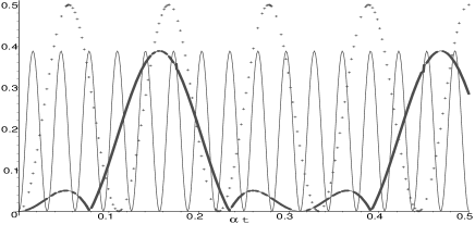
Figure 1: Concurrence function, $C_{onc}$, against $\alpha_{A}t$ in correspondence to $N=100$ and $r=1$ (point line), $r=10$ and $r=10^{-1}$ (bold line) respectively.

As clearly shown, varying the parameter $r$ the concurrence function always manifests a periodic oscillatory behaviuor immediately deducible taking into account the fact that, in the case under scrutiny, $C_{onc}(t)=2|c(t)|$. In particular we may state that, whatever $r$ is, there exist infinite values of $t$ in correspondence of which $C_{onc}(t)=0$ meaning that the central system is separable. It is worth emphasizing the remarkable circumstance that when $r=1$ the matrix element $c(t)$ at any time instant $t$ assumes its maximum value compatible with relation (5), that is $|c(t)|=\sqrt{b(t)d(t)}$. In order to verify the occurrence of such a saturation of the inequality (5) at any $t$, it is enough to put $r=1$ in eqs. (29)-(31). On the other hand, it happens that in correspondence to all the time instants such that $C_{onc}(t)=0$ also the diagonal matrix element $e(t)$ vanishes. This means that at these time instants all the conditions on the density matrix of two spins defining a pure state are verified Landau . Thus we may claim that when the two spins $A$ and $B$ are equally coupled to the spin bath, namely $r=1$, the condition $C_{onc}(t)=0$ not only reveals absence of entanglement in the central system but also guarantees that such two spin system is in a pure state. Looking indeed at eqs. (29)-(31) it is immediate to convince oneself that the two spins are periodically found in the initial state $|1^{A},-1^{B}\rangle$ or in the state $|-1^{A},1^{B}\rangle$ in which the role played by the two spins is exchanged. This behaviour is clearly illustrated in figure (2) where we compare the concurrence function with the temporal evolution of the probability of finding the state $|1^{A},-1^{B}\rangle$ and that of measuring the state obtained exchanging the two spins.

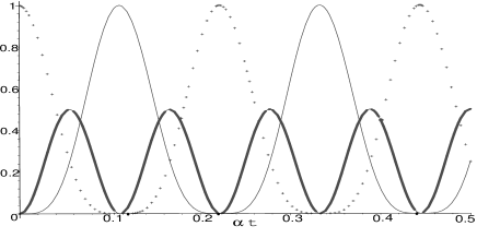
Figure 2: Concurrence function, $C_{onc}$,(bold line), probability of finding the state $|-1^{A},1^{B}\rangle$ (point line) and probability of finding the state $|1^{A},-1^{B}\rangle$ (continuous line), against $\alpha_{A}t$ and in correspondence to $N=100$ and $r=1$.

Let’s now examine how the system evolves starting from another initial condition of experimental interest that is

$$|\psi(0)\rangle=|1^{A},1^{B},\frac{N}{2},-\frac{N}{2},1\rangle$$ (34)

obtained leaving once again the bath in its ground state and preparing the preferred couple of spins in the state correspondent to the maximum values of $S_{z}^{(AB)}$. It is possible to prove that under this initial condition and assuming that the Hamiltonian model (19) is invariant under the permutation of $A$ with $B$ ($\alpha_{A}=\alpha_{B}\equiv\alpha$), the central system develops correlations when the time goes on. More in detail the temporal behaviour of $C_{\sigma_{x}\sigma_{x}}$ in this case is given by

$$C_{\sigma_{x}\sigma_{x}}(t)=\frac{N}{3N-2}\sin^{2}{\omega t}$$ (35)

where

$$\omega=2\sqrt{6N-4}\alpha$$ (36)

The maximum amount of correlation between $\sigma_{x}^{A}$ and $\sigma_{x}^{B}$ is obviously strictly related to the number of external spins populating the bath but, however, is larger than $\frac{1}{3}$ as immediately deducible by eq. (35). On the other hand, evaluating the concurrence function exploiting the results presented in section II yields

$$C_{onc}(t)=\max{[0,f_{N}(x)]}$$ (37)

where

$$f_{N}(x)=\frac{2N\sqrt{2N(N-1)}-N(3N-2)}{(3N-2)^{2}}x^{2}+$$ (38)

$$-\frac{2(N-2)\sqrt{2N(N-1)}}{(3N-2)^{2}}x+$$

$$+\frac{4(1-N)\sqrt{2N(N-1)}+N(3N-2)}{(3N-2)^{2}}$$

with $x\equiv\cos{\omega t}$ with $\omega$ given by eq. (36). It is easy to verify that $f_{N}(x)$ is not positive when $x\in[-1,1]$. Thus we may conclude that whatever $N$ is, the concurrence function $C_{onc}(t)$ is equal to zero at any time instant $t$. In other words, differently from the case before analyzed, under the hypotheses before discussed the concurrence function is equal to zero at any time instant $t$. Stated differently the correlations occurring in the central system at a generic time instant $t$, manifested throughout $C_{\sigma_{x}\sigma_{x}}(t)\neq 0$, have only a classical origin and therefore we say that such correlations are classical.

It is interesting to observe that this inability of the system to generate entanglement between the spins $A$ and $B$ when the system is prepared accordingly to eq. (34), is overcome simply breaking the symmetry condition $r=1$. This fact is clearly shown in figure (3) where we plot the two functions $C_{onc}(t)$ and $C_{\sigma_{x}\sigma_{x}}(t)$ in correspondence to $N=100$ and $r=10$. Thus for $r\neq 1$ the concurrence function remains zero for a given interval of time, then abruptly increases and once again falls to zero. This behaviour is then periodically recovered reaching maximum values of $C_{onc}(t)$ of experimental interest. We wish to remark that the evolution of the system in this case is characterized by intervals of time during which the system develops only classical correlations ($C_{onc}(t)=0$ and $C_{\sigma_{x}\sigma_{x}}(t)\neq 0$) and intervals of time where quantum correlations occur ($C_{onc}(t)\neq 0$).

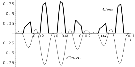
Figure 3: Covariance function $C_{\sigma_{x}\sigma_{x}}$ and concurrence $C_{onc}$ against $\alpha_{A}t$, in correspondence to $N=100$ and $r=10$

IV Conclusive remarks

In this paper we have analyzed the quantum dynamics of a system of $M$ Heisenberg coupled spins $\frac{1}{2}$ concentrating in particular on a couple of them and looking for the time evolution of entanglement developed between the two spins. We have demonstrated that it is possible to establish a conceptual and quantitative link between the concurrence function and easily measurable quantities only requiring that at a generic time instant $t$ the reduced density matrix describing the two spins of interest can be put in the simple form given by eq. (4). This circumstance not only allows the possibility of physically interpreting the concurrence function introduced by Wootters as an useful and powerful mathematical tool to estimate the degree of entanglement, but also suggests a direct way to measure it. The quantitative relation given by eq. (14) provides indeed the possibility of measuring the entanglement without reconstructing the state of the two spins. Examining in particular a specific physical system, namely the generalized spin star system discussed in section III, we have put into light that detecting the covariance function of the two commuting observables $\sigma_{x}^{A}$ and $\sigma_{x}^{B}$ directly provides the entanglement evolution get established between the two central spins. Exploiting the knowledge of the exact expression of the density matrix of the system, $\rho_{AB}(t)$, starting from an arbitrary initial condition, we have disclosed a rich dynamics. In particular we have envisaged physical conditions under which the two central spins are able to develop classical correlations only being in this case $C_{onc}(t)=0$ at any time instant $t$. At the same time we have found that slightly changing some parameters characterizing the system, quantum correlations appear.

References

- (1) D. Loss, D.P. Di Vincenzo, Phys. Rev. A 57, 120 (1998).
- (2) P. Karbach, J. Stolze, Phys. Rev. A 72, 030301(R) (2005).
- (3) V.V. Dobrovitski, H. A. DeRaedt, M. I. Katsnelson, B. N. Harmon Phys. Rev. Lett. 90, 210401 (2003).
- (4) Geza Toth, Phys. Rev. A 71, 010301(R) (2005).
- (5) F.M. Cucchietti, J. P. Paz, W. H. Zurek Phys. Rev. A 72, 052113 (2005).
- (6) G. Burkard, cond-mat/0409626.
- (7) D.D. Awschalom et al., Semiconductor Spintronics and Quantum Computation, Springer (Berlin 2002).
- (8) A. Imamoglu et al, Phys. Rev. Lett. 83, 4204 (1999).
- (9) M.C. Arnesen, S. Bose, V. Vedral Phys. Rev. Lett. 87, 017901 (2001).
- (10) Guo-Feng Zhang, Shu-Shen Li, Phys. Rev. A 72, 034302 (2005).
- (11) L.-A. Wu, S. Bandyopadhyay, M. S. Sarandy, D. A. Lidar Phys. Rev. A 72, 032309 (2005).
- (12) L. Zhou, H. S. Song, Y. Q. Guo, C. Li Phys. Rev. A 68, 024301 (2003).
- (13) A. Hutton, S. Bose, Phys. Rev. A 69, 042312 (2004).
- (14) S.D. Hamieh, M.I. Katsnelson, Phys. Rev. A 72, 032316 (2005).
- (15) Daniel C. Mattis, The theory of magnetism made simple, World Scientific Publishing Co. Pte. Ltd. (Singapore 2006)
- (16) J.S. Pratt, Phys. Rev. Lett. 93, 237205 (2004).
- (17) L.D. Landau, E.M. Lifsits, Quantum Mechanics
- (18) A. Peres, Phys. Rev. Lett. 77, 1413 (1996).
- (19) M. Horodecki et al., Phys. Lett. A 223 (1996).
- (20) W. K. Wootters Phys. Rev. Lett. 80, 2245-2248 (1998).
- (21) Ting Yu, J.H. Eberly Phys. Rev. Lett. 93, 140404 (2004).
- (22) Ting Yu, J.H. Eberly, quant-ph/0503089 (2005)
- (23) M. Yonac, T. Yu, J. H. Eberly, quant-ph/0602206 (2006).
- (24) Heinz-Peter Breuer, D. Burgarth, F. Petruccione Phys. Rev. B. 70, 045323 (2004).