Cooperating or Fighting with Decoherence
in the Optimal Control of Quantum Dynamics

Abstract

This paper explores the use of laboratory closed-loop learning control to either fight or cooperate with decoherence in the optimal manipulation of quantum dynamics. Simulations of the processes are performed in a Lindblad formulation on multilevel quantum systems strongly interacting with the environment without spontaneous emission. When seeking a high control yield it is possible to find fields that successfully fight with decoherence while attaining a good quality yield. When seeking modest control yields, fields can be found which are optimally shaped to cooperate with decoherence and thereby drive the dynamics more efficiently. In the latter regime when the control field and the decoherence strength are both weak, a theoretical foundation is established to describe how they cooperate with each other. In general, the results indicate that the population transfer objectives can be effectively met by appropriately either fighting or cooperating with decoherence.

I Introduction

Control over quantum dynamics phenomena is the focus of many theoretical Rice and Zhao (2000); Rabitz (2003); Shapiro and Brumer (2003) and experimentalWalmsley and Rabitz (2003); Brixner et al. (2001a) studies. Various control scenarios exist, including optimal controlPeirce et al. (1988); Kosloff et al. (1989), coherent controlShapiro and Brumer (1986), and STIRAP(Stimulated Raman Adiabatic Passage) controlGaubatz et al. (1990); Kobrak and Rice (1998). Increasing numbers of control experiments, including on complex systemsAssion et al. (1998); Bergt et al. (1999); Kunde et al. (2000); Bartels et al. (2000); Brixner et al. (2001b); Levis et al. (2001); Herek et al. (2002); Daniel et al. (2003), employ closed-loop optimal controlJudson and Rabitz (1992). Many of the control systems explored theoretically are restricted to pure state dynamics or the dynamics of isolated quantum systems. In practice, control field noiseGeremia et al. (2000); Rabitz (2002); Sola and Rabitz (2004) and decoherenceBlanchard et al. (2000); Braun (2001) inevitably will be present in the laboratory and the general expectation is that their involvement will be deleterious towards achieving control. Recent studies have investigated the effect of field noise and shown that controlled quantum dynamics can survive even intense field noise and possibly cooperate with it under special circumstancesShuang and Rabitz (2004). Decoherence of quantum dynamics in open systems, which often represents realistic situations, is a concern for control of atomic and molecular process, especially in condensed phases. Simulations have shown that it’s possible to use closed-loop learning control to suppress the effect of quantum decoherenceZhu and Rabitz (2003). Some investigations have been performed on laser control of population transfer in dissipative quantum systemOhtsuki et al. (2001); Kurkal and Rice (2002); Batista and Brumer (2002); Xu et al. (2004). Control of decoherence and decay of quantum states in open systems has also been exploredEberly (1998); Viola (2004). Decoherence was shown to possibly be constructive in quantum dynamicsPrezhdo (2000); Kendon and Tregenna (2004).

This paper considers the influence of decoherence (dissipation) upon the controlled dynamics of population transfer with the decoherence induced by interaction with the environment but spontaneous emission is not included. This regime arises, for example, in condensed phases where significant environmental interactions dominate the decoherence processes. The goal is to demonstrate that effective control of population transfer is possible in the presence of decoherence. It is naturally found that decoherence is deleterious to achieving control if a high yield is desired, however we also find that good control solutions can be found that achieve satisfactory yields. If a low yield is acceptable, then it is shown that decoherence even can be helpful and the control field can cooperate with the decoherence. This paper will investigate these phenomena numerically and analytically to illustrate the issues, and this work compliments an analogous study considering the influence of field noiseShuang and Rabitz (2004).

The dynamical equations and control formulation is presented in Section II. Simulations of closed-loop management of dynamics with decoherence is given in Sec.III. Section IV develops an analytical formulation to describe how the control field and the decoherence cooperate with each other when they are both weak. Finally, a brief summary of the findings is presented in Section V.

II The Model System

Realistic quantum systems in the laboratory often can not be fully described by a simple, fully certain Hamiltonian. Instead, almost all real systems are affected by dissipation, decoherence or noise, which can not be totally eliminated. The recent successes of closed-loop optimization algorithmsJudson and Rabitz (1992) operating in the laboratory demonstrate the capability of finding optimal, stable and robust solutions automaticallyAssion et al. (1998); Bergt et al. (1999); Kunde et al. (2000); Bartels et al. (2000); Brixner et al. (2001b); Levis et al. (2001); Herek et al. (2002); Daniel et al. (2003), even for very complex systems. The present work aims to support the continuing experiments by investigating the principles and rules of control in the presence of decoherence. In keeping with this goal, a simple model system will be investigated.

The effect of dissipation on controlled quantum dynamics will be explored in the context of population transfer in multilevel systems characterized by the dynamical equation of the reduced density matrix $\rho_{S}$

$$\frac{\partial\rho_{S}(t)}{\partial t} =-i[H_{0}-\mu E(t),\rho_{S}(t)]+\gamma\mathcal{F}\left\{\rho_{S}(t)\right\}\text{,}$$ (1a)

$$H_{0} =\sum_{\upsilon}\varepsilon_{\upsilon}\left|\upsilon\right\rangle\left\langle\upsilon\right|\text{,}$$ (1b)

where $$\left|\upsilon\right\rangle H_{0} \varepsilon_{\upsilon} \upsilon E(t)$$ is an eigenstate of the controlled system Hamiltonian , and is the associated -th field-free eigen-energy. The noise-free control field is taken to have the form

$$E(t) =s\left(t\right)\sum_{l}A_{l}\cos\left(\omega_{l}t+\theta_{l}\right)\text{,}$$ (2a)

$$s\left(t\right) =\exp\left[-\left(t-T/2\right)^{2}/2\sigma^{2}\right]\text{,}$$ (2b)

where $$\left\{\omega_{l}\right\} \left\{A_{l}\right\} \left\{\theta_{l}\right\} \mu$$ are the allowed resonant transition frequencies of the system, and off-resonant excitation are not included. The controls are the amplitudes and phases , and the control interacts with the system through the dipole operator . In the laboratory such control fields may be generated with programmable adaptive phase and amplitude femtosecond pulse shaping techniquesWefers and Nelson (1993); Weiner (2000).

In Eq.(1a) $\mathcal{F}\left\{\rho_{S}(t)\right\}$ is a functional which represents decoherence caused by the environment and $\gamma$ is a positive coefficient which indicates the strength of the decoherence and will be varied in this paper to study the effect of dissipation on the control of quantum dynamics. Various equations have been developedLindblad (1976); Yan (1998); Yan et al. (2000) to describe the interaction between a system and the environment. In this paper we take the Lindblad formLindblad (1976):

$$\mathcal{F}\left\{\rho_{S}(t)\right\}=\sum_{\left\{jn\right\}}\left(\mathcal{L}_{\left\{jn\right\}}\rho_{S}(t)\mathcal{L}_{\left\{jn\right\}}^{\dagger}-\frac{1}{2}\rho_{S}(t)\mathcal{L}_{\left\{jn\right\}}^{\dagger}\mathcal{L}_{\left\{jn\right\}}-\frac{1}{2}\mathcal{L}_{\left\{jn\right\}}^{\dagger}\mathcal{L}_{\left\{jn\right\}}\rho_{S}(t)\right)\text{,}$$ (3)

Here $\mathcal{L}_{\left\{jn\right\}}$ are bounded linear Lindblad operators acting on $\rho_{S}$ such that the norm of the operators, $\sum_{\left\{jn\right\}}\mathcal{L}_{\left\{jn\right\}}^{\dagger}\mathcal{L}_{\left\{jn\right\}},$ is finite. In the Lindblad equation, the Markovian and weak coupling approximations are made, and the normalization and positive definite nature of the reduced density matrix $\rho_{S}(t)$ is preserved.

In the model system studied here, the Lindblad operators in Eq.(3) are expressed phenomenologically asGardiner and Zoller (2000)

$$\mathcal{L}_{jn}=\sqrt{\Gamma_{jn}}\left|j\right\rangle\left\langle n\right|,\ j,n=0,1,...,N-1\text{,}$$ (4)

where $N$ is the number of levels and $\left|j\right\rangle$ are eigenstates of the isolated system Hamiltonian $H_{0}$. The coefficient $\Gamma_{jn}$, when multiplied by $\gamma$, specifies the transition rate between level $j$ and $n$. These rates depend on how the system and environment interact and will be chosen arbitrarily for the purposes of the general analysis here.

Inserting Eq.(4) into Eq.(3) produces the dynamical equation for the reduced density matrix of the multi-level system,

$$\frac{\partial\rho_{ll^{\prime}}(t)}{\partial t} =-i(\varepsilon_{l}-\varepsilon_{l^{\prime}})\rho_{ll^{\prime}}(t)-i\sum_{n=0}^{N-1}\left(\mu_{ln}\rho_{nl^{\prime}}(t)-\rho_{ln}(t)\mu_{nl^{\prime}}\right)E(t)+\gamma\mathcal{F}\left\{\rho_{S}(t)\right\}_{ll^{\prime}}\text{,}$$ (5a)

$$\mathcal{F}\left\{\rho_{S}(t)\right\}_{ll^{\prime}} =\delta_{ll^{\prime}}\sum_{n=0}^{N-1}\Gamma_{ln}\rho_{nn}(t)-\frac{1}{2}\sum_{n=0}^{N-1}\left(\Gamma_{nl}+\Gamma_{nl^{\prime}}\right)\rho_{ll^{\prime}}(t)\text{.}$$ (5b)

Closed-loop control simulations will be performed with model systems, but under the standard cost functionGeremia et al. (2000) realizable in laboratory circumstances:

$$J\left[E(t)\right] =\left|O\left[E(t),\gamma\right]-O_{T}\right|^{2}+\alpha F\text{,}$$ (6a)

$$F =\sum_{l}\left(A_{l}\right)^{2}\text{,}$$ (6b)

where $$O_{T}$$ is the target value (expressed as a percent yield) and

$$O\left[E(t),\gamma\right]=\text{Tr}[\rho(T_{f})O_{f}]$$ (7)

is the outcome produced by the trial field $E(t)$ under decoherence strength $\gamma$, and $F$ is the fluence of the control field whose contribution is weighted by the constant, $\alpha>0$. In the present work, $O_{f}=\left|\Psi_{f}\right\rangle\left\langle\Psi_{f}\right|$ is a projection operator for the population in a target state $\left|\Psi_{f}\right\rangle$.

III Numerical Simulations

To demonstrate how quantum optimal control can either fight or cooperate with decoherence, we perform four simulations with simple model systems. The first three simulations use the single path system in Figure (1a) which represents a model multi-level systemShore (1990) or a truncated nonlinear oscillatorLarsen and Bloembergen (1976); Wallraff et al. (2004); Dykman and Fistul (2005), while the last simulation uses the double-path system in Figure (1b). With the single path system, the first two models employ different decoherence coefficients $\Gamma_{ij}$ associated with nearest neighbor transitions in Eq.(5b). The third model allows as well for next nearest neighbor transitions. The fourth model with the double-path system shows how cooperation between decoherence and the control field can influence the transition path taken by the dynamics. The decoherence term doesn’t include spontaneous emission. All of the simulations employ closed-loop optimization with a Genetic AlgorithmGoldberg (1989) (GA), in keeping with common laboratory practice. Equation (6a) is the cost function used to guide the GA determination of the control field. The model parameters below are chosen to be illustrative of the controlled physical phenomena, and similar behavior was found for other choices as well.

III.1
Model 1

This model uses the simple 5-level system in Figure (1a) with eigenstates $\left|i\right\rangle$, $i=0,\cdots,4$ of the field free Hamiltonian $H_{0}$, having only nearest neighbor transitions with the frequencies $\omega_{01}=1.511$, $\omega_{12}=1.181$, $\omega_{23}=0.761$, $\omega_{34}=0.553$ in rad$\cdot$fs^-1, and associated transition dipole moments $\mu_{01}=0.5855$, $\mu_{12}=0.7079$, $\mu_{23}=0.8352$, $\mu_{34}=0.9281$ in $10^{-30}$ C$\cdot$m. The decoherence coefficients $\Gamma_{ij}$ in Eq.(5) are also non-zero only between nearest neighbor levels: $\Gamma_{01}=\Gamma_{10}=0.0895$, $\Gamma_{12}=\Gamma_{21}=0.1942$, $\Gamma_{23}=\Gamma_{32}=0.1209$, $\Gamma_{34}=\Gamma_{43}=0.2344$. The target time is $T=200$ fs, and the pulse width in Eq.(2b) is $\sigma=30$ fs. The control objective is to transfer population from the initially prepared ground state $\left|0\right\rangle$ to the final state $\left|4\right\rangle$, such that $O=\left|4\right\rangle\left\langle 4\right|$. In order to calibrate the strength of the decoherence, Table I shows the state population distributions when the system is only driven by various environmental interaction decoherence strengths. When $\gamma\geqslant 0.03$ fs^-1, decoherence is very strong as it drives more than 30% of the population out of ground state at $t=200$ fs.

To examine the influence of decoherence when seeking an optimal control field, first consider a high target yield (i.e., perfect control with the target yield set at $O_{T}=100\%$ in Eq.(6a)). The simulation results in Table II show that decoherence is always deleterious for achieving this target, but a good yield is still possible. In order to reveal the separate contributions of decoherence and the control field, Table II also shows the yield from the decoherence alone $O\left[E(t)=0,\gamma\right]$ without the control field being present and the yield from the control field alone $O\left[E(t),\gamma=0\right]$ without decoherence being present.

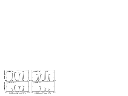
Figure 2: Power spectra of the control fields for model 1 aiming at a low yield of $O_{T}=5.0\%$ (Table III). $\gamma$ indicates the strength of decoherence (Eqs.(1) and (5)). The control field intensity generally decreases with the increasing decoherence strength reflecting cooperative effects.

If we accept a low control yield outcome, very different control behavior is found in the presence of decoherence. The results from optimizing Eq.(6a) are shown in Table III with various levels of decoherence for a target yield of $O_{T}=5.0\%$. The results in Table III clearly indicate that there is cooperation between the control field and the decoherence. For example, when $\gamma=0.03$ fs^-1, the outcome of the control field and decoherence together ($O[E(t),\gamma]=4.94\%$) is much larger than outcome from control field alone ($O\left[E(t),\gamma=0\right]=0.63\%$) or the decoherence alone ($O\left[E(t)=0,\gamma\right]=0.67\%$), and even larger than their sum ($1.30\%$). Table III also shows that the control process become more efficient with increasing decoherence strength ($\gamma$) as the fluence of the control field is reduced while driving the dynamics to the same target. The control field spectra at different decoherence strengths are depicted in Fig.2. The mechanism of cooperation between the control field and decoherence is not easy to identify from Fig.2. In the following simple model the decoherence coefficients $\Gamma_{ij}$ are specially selected to identify the mechanism of cooperation.

III.2
Model 2

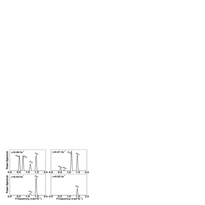
Figure 3: The same situation as Figure 2, but for model 2. Here the peaks corresponding to transitions involving higher quantum states disappear successively in keeping with the ability of decoherence to aid in meeting the desired physical goal.

This model is similar with model 1. The only difference is that the transition rates $\Gamma_{ij}$ in Eq.(5a) are chosen to increase monotonically: $\Gamma_{01}=\Gamma_{10}=0.03495$, $\Gamma_{12}=\Gamma_{21}=0.1242$, $\Gamma_{23}=\Gamma_{32}=0.3909$, $\Gamma_{34}=\Gamma_{43}=0.6344$. Table IV is the low target yield analog of Table III, but for model 2. Once again clear evidence is found for the optimal field cooperating with the decoherence. In order to deduce the mechanism of cooperation between the control field and the decoherence, Fig. 3 shows optimal control field spectra at different levels of decoherence. The control field consists of four peaks, corresponding to the four transitions between nearest neighbor levels. With increasing decoherence strength, $\gamma$, the peak intensities corresponding to transitions among the higher levels, become smaller, and successively disappear. This behavior shows that control field can be found to cooperate with decoherence and drive the dynamics more efficiently. As a result, the cooperation between the control field and environment becomes dramatic for $\gamma>0.03$ fs^-1. In this region the optimal field has essentially no amplitude at the $2\rightarrow 3$ and $3\rightarrow 4$ transition frequencies such that the field alone produces a vanishingly small yield, yet with the environment present the cooperation is very efficient. If we chose the decoherence coefficients $\Gamma_{ij}$ in Eq.(5a) decrease monotonically(not shown here), then with increasing decoherence strength, the peak intensities corresponding to transitions between the lower levels disappear successively. This behavior indicates a similar cooperation mechanism, but with a shift in the role of the various transitions.

III.3 Model 3

Model 3 is similar to model 1 except that two-quanta transitions are also allowed: $\omega_{02}=2.692$, $\omega_{13}=1.942$, $\omega_{24}=1.314$ in rad$\cdot$fs^-1, with transition dipole elements: $\mu_{02}=-0.1079$, $\mu_{13}=-0.1823$, $\mu_{24}=-0.2786$ in 10^-3 C$\cdot$m. We also assume that there are environmentally induced two-quanta transitions: $\Gamma_{02}=0.01099$, $\Gamma_{13}=0.1087$, $\Gamma_{24}=0.1346$. Table V shows the outcome from model 3 with a low yield target $O_{T}=10\%$. Once again, cooperation between decoherence and the control field is found, although to a lesser degree than in the earlier cases. The decrease in the degree of cooperation appears mainly to arise from the enhanced target value of $O_{T}=10\%$. As shown in model 1, eventually decoherence has a deleterious effect when aiming towards a sufficiently high yield. However, under special circumstances, such as decoherence breaking the symmetry of the Hamiltonian $H(t)$, decoherence could still have a beneficial role when seeking a high yield.

III.4 Model 4

Model  4 is the more complex two-path system in Figure 1(b). In this model, population can be transferred to the target state $\left|4\right\rangle$ along two separate pathways. The transition frequencies, decoherence coefficients and dipoles of the left path are the same as that of model 1; the right path has the distinct transition frequencies: $\omega_{01^{\prime}}=2.513,\omega_{1^{\prime}2^{\prime}}=1.346,\omega_{2^{\prime}3^{\prime}}=0.345,\omega_{3^{\prime}4}=0.162$ in rad$\cdot$fs^-1, decoherence coefficients: $\Gamma_{01^{\prime}}=\Gamma_{1^{\prime}0}=0.1164$, $\Gamma_{1^{\prime}2^{\prime}}=\Gamma_{2^{\prime}1^{\prime}}=0.0885$, $\Gamma_{2^{\prime}3^{\prime}}=\Gamma_{3^{\prime}2^{\prime}}=0.1557$, $\Gamma_{3^{\prime}4}=\Gamma_{43^{\prime}}=0.1280$ and dipole elements: $\mu_{01^{\prime}}=0.6525,\mu_{1^{\prime}2^{\prime}}=0.7848,\mu_{2^{\prime}3^{\prime}}=0.9023,\mu_{3^{\prime}4}=1.0322$ in $10^{-30}$ C$\cdot$m. For simplicity, only single quanta transitions are allowed along both paths.

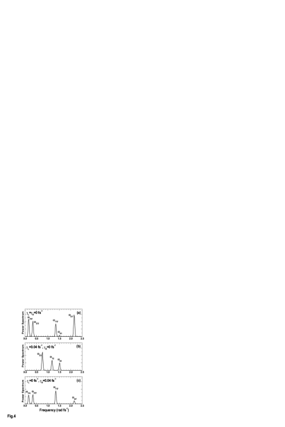
Figure 4: Power spectra of the control fields for model 4 (see panel (b) of Figure 1). The frequencies along the right path in Figure 1 are denoted with a prime to distinguish them from the left path. (a) No decoherence, (b) decoherence in the left path, (c) decoherence in the right path. In these low target yield cases the optimal field cooperates with the decoherence directing the dynamics to follow the associated path.

The results in Table VI show cooperation between the field and the decoherence in model 4 for a low target yield of $O_{T}=5\%$. Figure 4 shows the power spectra of the three optimal control fields in Table VI. Panel (a) indicates that in the case of no decoherence the control field primarily drives the system along the right path. When decoherence is present in the left path (panel (b)), the optimal control field chooses to drive the system dynamics along the left path in order to cooperate with the decoherence. The lack of a peak at $\omega_{34}$ in the latter case reflects the cooperation between the control field and the environment. Similarly, in panel (c), when decoherence is in the right path, the optimal field chooses to drive the system along the right path. These results clearly show that efficiently achieving the yield is the guiding principle dictating the nature of the control field and the mechanism in these cases. The cost function in Eq.(6) explicitly contains a fluence term which naturally guides the closed-loop control search towards efficient fields, and cooperating with decoherence is consistent with this goal. The common circumstance in the laboratory of having a fixed maximum fluence would produce similar behavior toward cooperating with decoherence when it’s beneficial.

IV Foundations for Cooperating with Decoherence

To illustrate the principle of how the control field can cooperate with decoherence consider excitation along a ladder (or chain) of nondegenerate transitions and energy levels, each linked only to its nearest neighbors as in models 1-2 in section III. One can also think of this system as a truncated nonlinear oscillatorLarsen and Bloembergen (1976); Wallraff et al. (2004); Dykman and Fistul (2005). The $N+1$ level system consists of an initially occupied ground state $\left|0\right\rangle$, $N-1$ intermediate states $\left|n\right\rangle$, and a final target state $\left|N\right\rangle$. The states are coupled with an external laser pulse having the nominal form in Eq.(2a). Both the control field and the decoherence are assumed to be weak in this section, corresponding to the low target yield cases in Section III.

Just as the parameter $\gamma$ characterizes the strength of decoherence, it is convenient to introduce a parameter $\lambda$ to characterize the strength of control field in Eq.(1a):

$$\frac{\partial\rho_{S}(t)}{\partial t}=-i[H_{0}-\mu\lambda E(t),\rho_{S}(t)]+\gamma\mathcal{F}\left\{\rho_{S}(t)\right\}\text{.}$$ (8)

In the analysis below we shall focus on the regime $\lambda\rightarrow 0$ and $\gamma\rightarrow 0$. Transforming the density matrix $\rho_{S}\left(t\right)$ to the interaction picture $\rho\left(t\right)=e^{-iH_{0}t}\rho_{S}\left(t\right)e^{iH_{0}t}$, or equivalently

$$\rho_{ll^{\prime}}=\left(\rho_{S}\right)_{ll^{\prime}}e^{-i\left(\varepsilon_{l}-\varepsilon_{l^{\prime}}\right)t}$$ (9)

produces

$$\frac{\partial}{\partial t}\rho\left(t\right) =\left[i\lambda\mathcal{L}_{I}\left(t\right)+\gamma\mathcal{F}\right]\rho\left(t\right)\text{,}$$ (10a)

$$\mathcal{L}_{I}\left(t\right)\rho\left(t\right) =\left[\mu^{\left(I\right)}(t)E(t),\rho\left(t\right)\right]\text{,}$$ (10b)

where $$\mu^{\left(I\right)}\left(t\right)=e^{-iH_{0}t}\mu e^{iH_{0}t} \mu_{kj}^{\left(I\right)}\left(t\right)=\mu_{kj}e^{-i\omega_{kj}t} \omega_{kj}=\varepsilon_{j}-\varepsilon_{k} \mathcal{F}$$, or in matrix form with . It is easy to show that the decoherence functional defined in Eq.(5b) is not changed under the transformation of Eq.(9). The solution of Eq.(10a) can be expressed formally as

$$\rho\left(T_{f}\right)=\exp_{+}\left[\int_{0}^{T_{f}}\left(i\lambda\mathcal{L}_{I}\left(t\right)+\gamma\mathcal{F}\right)dt\right]\rho\left(0\right)\text{,}$$ (11)

where $\exp_{+}$ is the time-ordering exponential operator. In order to explore the scaling with $\gamma$ and $\lambda$ we shall now introduce the first order Magnus approximationMagnus (1954), which ignores the time ordering , such that

$$\rho\left(T_{f}\right) \approx\exp\left[\int_{0}^{T_{f}}\left(i\lambda\mathcal{L}_{I}\left(t\right)+\gamma\mathcal{F}\right)dt\right]\rho\left(0\right)$$ (12a)

$$=\exp\left[\left(i\lambda\mathcal{E}+\gamma\mathcal{F}\right)T_{f}\right]\rho\left(0\right)\text{,}$$ (12b)

where $$\mathcal{E}$$ is a time-independent functional acting as

$$\mathcal{E}\rho=\left[W,\rho\right]$$ (13)

with the matrix $W$ defined as

$$W =\frac{1}{T_{f}}\int_{0}^{T_{f}}\mu^{\left(I\right)}\left(t\right)E\left(t\right)dt\text{,}$$ (14a)

$$W_{kj} =\frac{1}{T_{f}}\int_{0}^{T_{f}}\mu_{kj}e^{-i\omega_{kj}t}E\left(t\right)dt\approx\mu_{kj}\frac{\varepsilon\left(\omega_{kj}\right)}{T_{f}}\text{.}$$ (14b)

Here $$\epsilon\left(\omega\right)$$ denotes the spectrum of the control pulse:

$$\epsilon\left(\omega\right)=\int_{-\infty}^{\infty}E(t)e^{-i\omega t}dt=\sum_{l=1}^{M}A_{l}\left[g\left(\omega-\omega_{l}\right)e^{i\theta_{l}}+g\left(\omega+\omega_{l}\right)e^{-i\theta_{l}}\right]\text{,}$$ (15)

with $g\left(\omega\right)$ being the Fourier transform of the shape function $s(t)$ in Eq.(2b). The first order Magnus approximation suffices in the ”impulse limit” of a sufficiently short pulsePechukas and Light (1966).

It’s convenient to introduce double bracket notationMukamel (1995) where the ket $\left|\left.jk\right\rangle\right\rangle$ denotes the Liouville space vector representing the Hilbert space operator $\left|j\right\rangle\left\langle k\right|$ and the bra $\left\langle\left\langle jk\right.\right|$ as the Hermitian conjugate to $\left|\left.jk\right\rangle\right\rangle$: $\left\langle\left\langle jk\right.\right|\equiv\left(\left|\left.jk\right\rangle\right\rangle\right)^{\dagger}\equiv\left|k\right\rangle\left\langle j\right|$. From Eqs.(7) and (12b), the outcome from applying the control field can be expanded and rewritten as

$$O\left[E\left(t\right),\gamma\right] =\left\langle\left\langle NN\right.\right|\exp\left[\left(i\lambda\mathcal{E}+\gamma\mathcal{F}\right)T_{f}\right]\left|\left.00\right\rangle\right\rangle$$ (16a)

$$=\sum_{k=0}^{\infty}\left\langle\left\langle NN\right.\right|\left(i\lambda\mathcal{E}+\gamma\mathcal{F}\right)^{k}\mathbf{P}^{k}\left(T_{f}\right)\left|\left.00\right\rangle\right\rangle\text{,}$$ (16b)

where the functional $$\mathbf{P}$$ is defined by:

$$\mathbf{P}\left[f\right]\left(t\right) =\int_{0}^{t}f\left(t_{1}\right)dt_{1}$$ (17a)

$$\mathbf{P}^{k}\left[f\right]\left(t\right) =\int_{0}^{t}dt_{1}\int_{0}^{t_{1}}dt_{2}\cdots\int_{0}^{t_{k-1}}dt_{k}f\left(t_{k}\right)\text{.}$$ (17b)

It is easy to verify that $$P^{k}\left[f\right]\left(t\right)=\frac{t^{k}}{k!} f(t)\equiv 1$$ for the identity function .

IV.1 Dynamics Driven by the Control Field Alone

When there is no decoherence, the yield from the control field is

$$O\left[E\left(t\right),0\right]=\sum_{k=0}^{\infty}\frac{T_{f}^{k}}{k!}\left\langle\left\langle NN\right.\right|\left(i\mathcal{E}\right)^{k}\left|\left.00\right\rangle\right\rangle\lambda^{k}\text{.}$$ (18)

The system yield can also be described in Hilbert space by

$$O\left[E\left(t\right),0\right]=\left|\left\langle N\right|e^{iWT_{f}\lambda}\left|0\right\rangle\right|^{2}=\left|\sum_{k=0}^{\infty}\frac{T_{f}^{k}}{k!}\left\langle N\right|\left(iW\right)^{N}\left|0\right\rangle\lambda^{k}\right|^{2}\text{.}$$ (19)

For a ladder system, $W$ is a tridiagonal matrix. When $\lambda\rightarrow 0$, we only need to keep the first non-zero terms of Eq.(19),

$$O\left[E\left(t\right),0\right]\approx\left|\frac{T_{f}^{N}}{N!}\left\langle N\right|\left(iW\right)^{N}\left|0\right\rangle\right|^{2}\lambda^{2N}=\frac{T_{f}^{2N}}{N!^{2}}T_{0N}^{2}\lambda^{2N}\text{,}$$ (20)

where the coherent transition elements $T_{mn}$ are defined as

$$T_{mn} =\left|\left\langle m\right|W^{n-m}\left|n\right\rangle\right|={\displaystyle\prod\limits_{k=m+1}^{n}}\left|W_{k,k-1}\right|={\displaystyle\prod\limits_{k=n}^{m}}\Omega_{k}\text{,}$$ (21a)

$$\Omega_{k} =\left|W_{k,k-1}\right|=\mu_{k,k-1}\frac{\left|\varepsilon\left(\omega_{k,k-1}\right)\right|}{T_{f}}\text{.}$$ (21b)

By comparing Eqs.(18) and (19), we know that the first non-zero term in Eq.(18) is $$k=2N$$

$$O\left[E\left(t\right),0\right]\approx\frac{T_{f}^{2N}}{2N!}\left\langle\left\langle NN\right.\right|\left(i\mathcal{E}\right)^{2N}\left|\left.00\right\rangle\right\rangle\lambda^{2N}\text{,}$$ (22)

and the following equality holds:

$$\left\langle\left\langle NN\right.\right|\mathcal{E}^{2N}\left|\left.00\right\rangle\right\rangle=C_{2N}^{N}T_{0N}^{2}\text{.}$$ (23)

The extension of the above equality to additional matrix elements is straightforward,

$$\left\langle\left\langle n+m,n+m\right.\right|\left(i\mathcal{E}\right)^{2m}\left|\left.nn\right\rangle\right\rangle=C_{2m}^{m}T_{n,n+m}^{2}\text{.}$$ (24)

Finally, the lowest order non-zero outcome from applying the control field without decoherence is

$$O\left[E\left(t\right),0\right]=\lambda^{2N}\frac{T_{f}^{2N}}{N!^{2}}T_{0N}^{2}\text{.}$$ (25)

IV.2 Dynamics Driven by Environmental Decoherence Alone

For simplicity, the decoherence is assumed to only induce transitions between nearest neighbor levels in the system, so that the decoherence matrix $\Gamma$ is tridiagonal with elements

$$\Gamma_{ij}=\left\langle\left\langle ii\right.\right|\mathcal{F}\left|\left.jj\right\rangle\right\rangle\text{,}$$ (26)

and $\Gamma$ plays a similar role as the dipole matrix. Decoherence can also drive the system from the initial state to the target state, at least to some degree, when there is no external field. The outcome due to environmental decoherence without the control field is

$$O\left[0,\gamma\right]=\sum_{k=1}^{\infty}\frac{T_{f}^{k}}{k!}\left\langle\left\langle NN\right.\right|\mathcal{F}^{k}\left|\left.00\right\rangle\right\rangle\gamma^{k}\text{.}$$ (27)

It is easy to obtain the following decoherence transition elements,

$$\left\langle\left\langle n+m,n+m\right.\right|\mathcal{F}^{m}\left|\left.nn\right\rangle\right\rangle=\prod_{k=1}^{m}\gamma_{n+k}\text{,}$$ (28)

where $\gamma_{k}$ is the $k$-th decoherence-induced transition rate between the nearest neighbor levels,

$$\gamma_{k}=\Gamma_{k+1,k}\text{.}$$ (29)

If the decoherence coupling is weak, $\gamma\rightarrow 0$, only the lowest non-zero term of Eq.(27) is needed,

$$O\left[E\left(t\right)=0,\gamma\right] \approx\frac{T_{f}^{N}}{N!}\left\langle\left\langle NN\right.\right|\mathcal{F}^{N}\left|\left.00\right\rangle\right\rangle\gamma^{N}$$ (30a)

$$=\gamma^{N}\frac{T_{f}^{N}}{N!}{\displaystyle\prod\limits_{k=1}^{N}}\gamma_{k}\text{,}$$ (30b)

which corresponds to a transition path $$\left|\left.00\right\rangle\right\rangle\rightarrow\left|\left.11\right\rangle\right\rangle\rightarrow\cdots\rightarrow\left|\left.NN\right\rangle\right\rangle$$.

IV.3 Cooperation between the Control Field and Decoherence

Consider the case where the control field and environmental decoherence are present simultaneously, so that the outcome is described by Eq.(12b). If the control field and decoherence are both weak, the perturbation approximation can be used again. Strong cooperation between the control field (Eq.(25)) and decoherence (Eq.(30b)) is expected when their contributions to the outcome are the same order, which corresponds to

$$\gamma=\lambda^{2}\text{.}$$ (31)

Then the perturbative solution $\rho\left(t\right)$ has the property

$$\rho_{mn}\left(t\right)\sim\lambda^{m+n}\text{.}$$ (32)

$\rho\left(T_{f}\right)$ in Eq.(12b) is the solution of following equation

$$\frac{\partial\rho\left(t\right)}{\partial t}=\left(i\lambda\mathcal{E}+\lambda^{2}\mathcal{F}\right)\rho\left(t\right)\text{,}$$ (33)

expressed explicitly as

$$\frac{\partial\rho_{ll^{\prime}}}{\partial t}\approx i\lambda\left(W_{l,l-1}\rho_{l-1,l^{\prime}}-\rho_{l,l^{\prime}-1}W_{l^{\prime}-1,l^{\prime}}\right)+\lambda^{2}\delta_{ll^{\prime}}\Gamma_{l,l-1}\rho_{l-1,l-1}\text{,}$$ (34)

where the terms higher than $\lambda^{l+l^{\prime}}$ are neglected. The last term of Eq.(34) represents the effect of decoherence which only drives transitions of the type $\left|\left.l-1,l-1\right\rangle\right\rangle\rightarrow\left|\left.ll\right\rangle\right\rangle$. If a high control yield is expected and the perturbation theory approximation is invalid, all of the decoherence terms in Eq.(5b) have to be considered, where some terms will interact destructively with the control field induced dynamics,

$$\left(\mathcal{F}\rho\right)_{ll^{\prime}}=\delta_{ll^{\prime}}\Gamma_{l,l-1}\rho_{l-1,l-1}+\delta_{ll^{\prime}}\Gamma_{l,l+1}\rho_{l+1,l+1}-\frac{1}{2}\left(\Gamma_{l-1,l}+\Gamma_{l+1,l}+\Gamma_{l^{\prime}-1,l^{\prime}}+\Gamma_{l^{\prime}+1,l^{\prime}}\right)\rho_{ll^{\prime}}\text{.}$$ (35)

Here it’s the first term that cooperates with the control field.

The outcome from both the control field and decoherence is

$$O\left[E\left(t\right),\gamma\right] =\left\langle\left\langle NN\right.\right|\exp\left[\left(\lambda i\mathcal{E}+\lambda^{2}\mathcal{F}\right)T_{f}\right]\left|\left.00\right\rangle\right\rangle$$ (36a)

$$=\sum_{k=1}^{\infty}\left\langle\left\langle NN\right.\right|\left[\lambda i\mathcal{E}\mathbf{P}\left(T_{f}\right)+\lambda^{2}\mathcal{F}\mathbf{P}\left(T_{f}\right)\right]^{k}\left|\left.00\right\rangle\right\rangle\text{.}$$ (36b)

Expanding the above equation and keeping only terms of order $$\lambda^{2N}$$, we get the perturbation approximation for the outcome,

$$O\left[E\left(t\right),\gamma\right]\approx\lambda^{2N}\sum_{m=0}^{N}\sum_{0\leq n_{1}<\cdots<n_{m}<N}A\left(n_{1},n_{2},\cdots,n_{m}\right)\text{,}$$ (37)

with $A\left(n_{1},n_{2},\cdots,n_{m}\right)$ given by

$$A\left(n_{1},n_{2},\cdots,n_{m}\right)=\mathbf{P}^{2N-m}\left(T_{f}\right)\left\langle\left\langle NN\right.\right|\left(i\mathcal{E}\right)^{2\left(N-n_{m}\right)}\left|\left.n_{m}n_{m}\right\rangle\right\rangle\\ \times{\displaystyle\prod\limits_{k=1}^{m}}\left\langle\left\langle n_{k}n_{k}\right.\right|\left(i\mathcal{E}\right)^{2\left(n_{k}-n_{k-1}-1\right)}\left|\left.n_{k-1}+1,n_{k-1}+1\right\rangle\right\rangle\left\langle\left\langle n_{k-1}n_{k-1}\right.\right|\mathcal{F}\left|\left.n_{k-1}+1,n_{k-1}+1\right\rangle\right\rangle\text{,}$$ (38)

describing the contribution of the paths in which the decoherence operator $\mathcal{F}$ drives the system from state $\left|\left.n_{k}-1,n_{k}-1\right\rangle\right\rangle$ to $\left|\left.n_{k},n_{k}\right\rangle\right\rangle$, and the control field operator $\mathcal{E}$ drives the system from state $\left|\left.n_{k}+1,n_{k}+1\right\rangle\right\rangle$ to $\left|\left.n_{k+1}n_{k+1}\right\rangle\right\rangle$. Substituting Eqs.(24) and (28) into Eq.(38), we have

$$A\left(n_{1},n_{2},\cdots,n_{m}\right) =\frac{T_{f}^{2N-m}}{\left(2N-m\right)!}C_{2\left(N-n_{m}-1\right)}^{N-n_{m}-1}{\displaystyle\prod\limits_{k=1}^{m}}T_{n_{k-1}+1,n_{k}}^{2}C_{2\left(n_{k}-n_{k-1}-1\right)}^{n_{k}-n_{k-1}-1}$$ (39a)

$$=T_{0N}^{2}\frac{T_{f}^{2N-m}}{\left(2N-m\right)!}C_{2\left(N-n_{m}-1\right)}^{N-n_{m}-1}{\displaystyle\prod\limits_{k=1}^{m}}\frac{\gamma_{n_{k}}}{\Omega_{n_{k}}^{2}}C_{2\left(n_{k}-n_{k-1}-1\right)}^{n_{k}-n_{k-1}-1}\text{.}$$ (39b)

If each term in Eq.(2a) is only resonant with a single transition,

$$\omega_{n}\approx\varepsilon_{n+1}-\varepsilon_{n}\text{,}$$ (40)

using the RWAShore (1990) (Rotating Wave Approximation) we can drop all non-resonant terms in Eq.(10a),

$$\mu^{\left(I\right)}(t)E(t)\approx s\left(t\right)H_{F}\text{.}$$ (41)

The time-independent $H_{F}$ matrix elements are

$$\left(H_{F}\right)_{kj}=\mu_{j}A_{j}\delta_{k,j+1}+\mu_{k}A_{k}\delta_{k+1,j}\text{.}$$ (42)

Here, $\mu_{k}=\mu_{k,k-1}$ denotes the $k$-th dipole element between the nearest levels. The operator $\mathcal{L}_{I}\left(t\right)$ commutes with itself at different times implying that the Magnus approximation is valid in the present circumstance under the RWA, and it’s easy to get Eq.(39b) with $\Omega_{k}$ being

$$\Omega_{k}=\mu_{k}A_{k}\frac{T_{e}}{T_{f}}\text{,}$$ (43)

defining the effective pulse duration as

$$T_{e}=\int_{0}^{T_{f}}s\left(t\right)dt\text{.}$$ (44)

It is also easy to show that the outcome of Eq.(37) can be decomposed into a linear combination of contributions from the field component intensity $A_{j}^{2}$ and the decoherence transition coefficients $\gamma_{j}$,

$$O\left[E\left(t\right),\gamma\right]=A_{j}^{2}F_{1j}+\gamma_{j}F_{2j}\text{,}$$ (45)

where $F_{1j}$ and $F_{2j}$ are functions independent of $A_{j}$ and $\gamma_{j}$, respectively. There is clearly cooperation between $A_{j}$ (a coherently driven transition) and $\gamma_{j}$ (a decoherently driven transition). For example, the outcome for a two level system is

$$\rho_{11}\left(T_{f}\right)=\left(\mu_{1}A_{1}\right)^{2}T_{e}^{2}+\gamma_{1}T_{f}\text{,}$$ (46)

and the outcome for a three level system is

$$\rho_{22}\left(T_{f}\right)=\frac{1}{4}\left(\mu_{1}A_{1}\mu_{2}A_{2}\right)^{2}T_{e}^{4}+\frac{1}{3}\left(\mu_{1}A_{1}\right)^{2}\gamma_{2}T_{e}^{2}T_{f}+\frac{1}{3}\left(\mu_{2}A_{2}\right)^{2}\gamma_{1}T_{e}^{2}T_{f}+\frac{1}{2}\gamma_{1}\gamma_{2}T_{f}^{2}\text{.}$$ (47)

The objective cost function in Eq.(6a) can be written in terms of the contributions from each specific control field intensity $A_{j}^{2}$,

$$J\left(A_{j}\right)=\left(A_{j}^{2}F_{1j}+\gamma_{j}F_{2j}-O_{T}\right)^{2}+\alpha A_{j}^{2}+\alpha\sum_{k\neq j}A_{k}^{2}\text{.}$$ (48)

Here, $F_{1j}$ and $F_{2j}$ are independent of both $A_{j}$ and $\gamma_{j}$. It is easy to show that the condition for optimizing Eq.(48) with respect to $A_{j}$ is

$$A_{j}^{2}F_{1j}+\gamma_{j}F_{2j}=O_{T}-\frac{\alpha}{2F_{1j}}\text{,}$$ (49)

The latter equation indicates that the contribution from decoherence can beneficially act to decrease the required amplitude of the optimal control field to attain the same yield.

V Conclusions

Various impacts of decoherence upon quantum control are explored in this paper. Numerical simulations from several cases indicate that control fields can be found that either cooperate with or fight against decoherence, depending on the circumstances. Two extreme cases of high and low target yield are chosen to illustrate distinct control behavior in the presence of decoherence: (a) the control field can fight against decoherence effectively when a high yield is desired, while (b) in the case of a low target yield, the control field can even cooperate with decoherence to drive the dynamics while minimizing the control fluence.

Four models were studied and a first-order perturbation theory of the weak control and decoherence limitis presented in this paper. Models 1 and 2 considered the control of the same system in different decoherence environments. Both cases show clear cooperation between the control field and the decoherence driven dynamics for low target yield. The detailed mechanistic role of decoherence can be subtle as indicated in model 1, although the final physical impact may be simple to understand. Model 2 clearly identified the role of decoherence by setting up a special structured interaction between the system and the environment. Although the conclusions in this paper are based on simple physical models with the Lindblad equation, similar behavior is expected for other systems and formulations of decoherence. The findings in this work are parallel with an analogous studyShuang and Rabitz (2004) on the role of control noise. These work aim to provide a better foundation to understand the physical processes at work when using closed-loop optimization in the laboratory, even in cases of significant noise and decoherence.

Table I. Population distribution of the single path model 1 when the system is only driven by interaction with the environment.

	Population in the state (%)
$\gamma\ ^{a}$(fs-1)	0	1	2	3	4
0.05	52.8	25.5	14.6	4.64	2.39
0.03	65.0	22.7	9.65	1.98	0.67
0.01	84.8	12.7	2.25	0.17	0.02
0.00	100	0	0	0	0

^a Strength of decoherence, refer to Eqs.(1) and Eq.(5)

Table II. Optimal control fields fighting against decoherence with model 1 for the highest possible objective yield of $O_{T}=100\%$.

$\gamma$(fs-1)	$O\left[E(t)=0,\gamma\right]^{a}$(%)	$O\left[E^{op}(t),\gamma=0\right]^{b}$(%)	$O\left[E^{op}(t),\gamma\right]^{c}$(%)	$O\left[E_{0}^{op}(t),\gamma\right]^{e}$(%)	$F\;^{d}$
0.05	2.39	97.58	34.90	34.58	0.071
0.03	0.67	98.43	46.61	46.42	0.067
0.01	0.02	98.65	72.90	72.79	0.066
0.00	0.00	98.53	98.53	98.53	0.064

^a Yield from decoherence alone without a control field

^b Yield arising from the control field without decoherence, but the control field is determined in the presence of decoherence at the specified value of $\gamma$.

^c Yield from the the optimal control field in the presence of decoherence, Eq.(7).

^d Fluence of the control field.

^e Yield from decoherence and the field optimized with zero decoherence.

Table III. Yields from optimal control fields with different levels of decoherence in the case of model 1 for a low objective yield of $O_{T}=5.0\%$.

$\gamma$(fs-1)	$O\left[E(t)=0,\gamma\right]^{a}$(%)	$O\left[E^{op}(t),\gamma=0\right]^{b}$(%)	$O\left[E^{op}(t),\gamma\right]^{c}$(%)	$F\;^{d}$
0.05	2.39	2$\times 10^{-4}$	4.92	4.08$\times 10^{-3}$
0.03	0.67	0.63	4.94	8.17$\times 10^{-3}$
0.01	0.02	3.01	4.96	1.23$\times 10^{-2}$
0.00	0.0	4.96	4.96	1.39$\times 10^{-2}$

^a,b,c,d refer to Table II.

Table IV. Optimal control with decoherence for model 2 with a low objective yield of $O_{T}=5.0\%$.

$\gamma$(fs-1)	$O\left[E(t)=0,\gamma\right]^{a}$(%)	$O\left[E^{op}(t),\gamma=0\right]^{b}$(%)	$O\left[E^{op}(t),\gamma\right]^{c}$(%)	$F\;^{d}$
0.05	2.2	7.69$\times 10^{-12}$	4.98	2.07$\times 10^{-3}$
0.03	0.71	2.51$\times 10^{-9}$	5.08	5.94$\times 10^{-3}$
0.01	0.03	0.52	4.90	1.23$\times 10^{-2}$
0.00	0.0	4.96	4.96	1.40$\times 10^{-2}$

^a,b,c,d refer to Table II.

Table V. Optimal control with decoherence for model 3 with a low objective yield of $O_{T}=10.0\%$.

$\gamma$(fs-1)	$O\left[E(t)=0,\gamma\right]^{a}$(%)	$O\left[E^{op}(t),\gamma=0\right]^{b}$(%)	$O\left[E^{op}(t),\gamma\right]^{c}$(%)	$F\;^{d}$
0.05	5.24	3.49	9.92	1.03$\times 10^{-2}$
0.03	2.08	4.73	10.00	1.17$\times 10^{-2}$
0.01	0.19	10.06	10.00	1.84$\times 10^{-2}$
0.00	0.0	10.00	10.00	1.70$\times 10^{-2}$

^a,b,c,d refer to Table II.

Table VI. Yield attained from the optimal field for model 4 with the low objective yield of $O_{T}=5\%$.

$\gamma=(\gamma_{L},\gamma_{R})^{e}$(fs-1)	$\left\langle O\left[E(t)=0,\gamma\right]\right\rangle_{N}{}^{a}$(%)	$O\left[E^{op}(t),\gamma=0\right]^{b}$(%)	$\left\langle O\left[E^{op}(t),\gamma\right]\right\rangle^{c}$(%)	$F\ ^{d}$
0.00,0,00	0.00	4.99	4.99	1.18$\times 10^{-2}$
0.04,0.00	1.42	1.34$\times 10^{-4}$	4.92	6.20$\times 10^{-3}$
0.00,0.04	0.85	0.33	4.95	5.98$\times 10^{-3}$

^a,b,c,d refer to Table II.

^e $\gamma_{L}$,$\gamma_{R}$: Decoherence strength in the left and right paths, respectively;

Figure 1: Two multilevel quantum systems used to investigate the impact of decoherence on optimally controlled dynamics. (a) The five level single path system used for simulations with models 1–3 in Sections III.A–III.C, respectively. Models 1 and 2 only allow for single quanta transitions (solid arrows) while model 3 allows both single and double quanta transitions (dashed arrows). (b) The double-path system for model 4 in Section 3.D.