Correcting low-frequency noise with continuous measurement

Abstract

Low-frequency noise presents a serious source of decoherence in solid-state qubits. When combined with a continuous weak measurement of the eigenstates, the low-frequency noise induces a second-order relaxation between the qubit states. Here we show that the relaxation provides a unique approach to calibrate the low-frequency noise in the time-domain. By encoding one qubit with two physical qubits that are alternatively calibrated, quantum logic gates with high fidelity can be performed.

Solid-state quantum devices have been demonstrated to be promising systems for quantum information processing NielsenBook . A key factor that affects the scalability of such devices is decoherence Gottesman ; KnillNature2005 . The low-frequency noise WeissmanPMP1988 was shown to be a serious source of decoherence and is ubiquitous in solid-state systems such as single-electron tunneling devices and superconducting qubits SimmondsPRL2004 ; WellstoodAPL2004 ; vanHarlingenPRB2004 ; AstafievPRL2004 ; ZorinPRB1996 and quantum optical systems Wineland2003 . Numerous theoretical and experimental works were devoted to the study of the physical origin of the low-frequency noise TheoryNoise . It has been widely accepted that the low-frequency noise features a spectrum of $1/f^{\alpha}$ with $\alpha\in[1,2]$ and a finite band width. Recently, several approaches were studied to control the decoherence from low-frequency noise, including the dynamical control technique NakamuraPRL2002 ; CollinPRL2004 ; ShiokawaPRA2004 ; GutmannPRA2005 ; FalciPRA2004 ; FaoroPRL2004 and circuit designs at the degenaracy point VionScience2002 ; MakhlinPRL2004 .

In the degeneracy point approach VionScience2002 , the low-frequency noise only induces off-diagonal coupling which is much weaker than the energy separation between the qubit states. Because of its low-frequency nature and the large energy separation, this coupling can not generate transition between the qubit states. Decoherence of the qubit is due to the second-order coupling between the noise and the qubit and is significantly suppressed MakhlinPRL2004 . This scenario, however, is changed when the qubit is continuously monitored by a detector. The measurement, together with the low-frequency noise, generates non-trivial dynamics for the qubit.

Continuous measurement is a useful tool for studying stochastic quantum evolution and was first explored in the context of quantum optics GardinerBook . Well-known applications of this technique include homodyne detection of an optical field in a cavity and measurement of the small displacement of a quantum harmonic oscillator CavesPRA1987 ; WisemanPRL1993 ; DohertyPRA1999 ; OreshkovPRL2005 . Recently, continuous measurement was adapted to solid-state systems such as quantum point contact and single-electron transistor to study the effect of detector’s back action on a qubit KorotkovPRB2001 ; MeasurementQubit . During a continuous measurement, the detector couples weakly with the measured system and only slightly perturbs the system. The measurement record contents a large contribution from the back action noise of the detector and a small contribution from the measured system. Meanwhile, the back action noise modifies the intrinsic dynamics of the measured system and can result in interesting phenomena.

In this paper, we study the dynamics of a continuously monitored qubit at the degeneracy point VionScience2002 ; MakhlinPRL2004 , where the detector measures the eigenstates of the qubit. Assisted by the measurement, the off-diagonal coupling of the low-frequency noise induces relaxation between the qubit states in addition to dephasing. It can be shown that the rate of the relaxation depends on the rate of the measurement linearly and depends on the magnitude of the noise quadratically. This stochastic process can be studied numerically in the quantum Bayesian formalism KorotkovPRB2001 and a real-time characterization of the low-frequency noise can be achieved from the measured switchings between the eigenstates of the qubit. We show that by using the measurement record to calibrate the noise, high fidelity quantum logic operations can be performed. This presents a novel approach to suppress the decoherence of the qubit due to the low-frequency noise.

Consider a qubit with an energy separation $2\hbar E_{z}$ between the states $|0\rangle$ and $|1\rangle$. At the degeneracy point, the noise induces off-diagonal coupling $\hbar\delta V$. The qubit Hamiltonian is

$$H_{0}=\hbar\left(\begin{array}[]{cc}-E_{z}&\delta V\\ \delta V&E_{z}\end{array}\right).$$ (1)

For low-frequency noise with $\langle|\frac{\partial\delta V}{\partial t}/\delta V|\rangle\ll 2E_{z}$ and $|\delta V|\ll 2E_{z}$, the energy separation prevents the transition between the qubit states and partially protects the qubit from decoherence. The noise causes dephasing by a second-order coupling as $H_{0}\approx\hbar(E_{z}+\delta V^{2}/4E_{z})\sigma_{z}$ with a noise spectrum $\left(\frac{\delta V^{2}}{4E_{z}}\right)_{\omega}^{2}$ MakhlinPRL2004 . Here $\sigma_{z,x}$ are the Pauli matrices of the qubit.

A measurement of the eigenstates of the qubit is performed with the detector current $I_{0}$ for the state $|0\rangle$ and $I_{1}$ for the state $|1\rangle$. The detector noise is described by a white noise spectrum $S_{I}$ which determines the measurement rate $\Gamma_{m}=\Delta I^{2}/4S_{I}$, the rate at which the qubit states can be resolved by the measurement, with $\Delta I=|I_{0}-I_{1}|$. For a continuous measurement, we have $\Delta I\ll(I_{0}+I_{1})/2$ and $\Gamma_{m}\ll\sqrt{E_{z}^{2}+\delta V^{2}}$. Hence, the measurement only slightly perturbs the qubit on the time scale of $1/2E_{z}$.

By averaging over all the trajectories of the continuous measurement, the master equation of the qubit can be written as GardinerBook

$$\frac{\partial\bar{\rho}}{\partial t}=-\frac{i}{\hbar}[H_{0},\,\bar{\rho}]-\frac{\Gamma_{m}}{4}[\sigma_{z},\,[\sigma_{z},\,\bar{\rho}]],$$ (2)

where $\bar{\rho}$ is the density matrix with the ensemble average. The last term in Eq.(2) describes the dephasing of the qubit due to the detector’s back action noise. The low-frequency noise can be treated as a perturbation in the above master equation. To second-order approximation, the evolution of the qubit can be derived and the probability of the state $|0\rangle$ follows $\partial\bar{\rho}_{00}/\partial t=-(\bar{\rho}_{00}-1/2)/\tau_{a}$ with a decay rate

$$\tau_{a}^{-1}=\frac{4\delta V^{2}\Gamma_{m}}{4E_{z}^{2}+\Gamma_{m}^{2}}$$ (3)

proportional to the measurement rate. The stationary state of the qubit for $t\gg\tau_{a}$ has $\bar{\rho}_{00}^{s}=\bar{\rho}_{11}^{s}=1/2$ and $\bar{\rho}_{01}^{s}=\bar{\rho}_{10}^{s}=0$ which is a mixture of the states $|0\rangle$ and $|1\rangle$ with equal probability. The information of the initial state of the qubit is lost because of the measurement. Hence, starting from an initial state $|0\rangle$, a switching to the state $|1\rangle$ can occur in the presence of the continuous measurement. Without the measurement at $\Gamma_{m}=0$, $\tau_{a}^{-1}=0$ and the switching can not occur. Note that in the limit of strong coupling between the detector and the qubit with $\Gamma_{m}\gg E_{z}$, the qubit dynamics is dominated by the quantum Zeno effect where fast measurement prevents the relaxation of the qubit.

In reality, selective quantum trajectories determined by the stochastic quantum master equation are recorded instead of the ensemble average. For the selective process, the switching between the qubit states occurs with the rate $\tau_{jp}^{-1}=\tau_{a}^{-1}/2$. Here the reduction of the rate by a factor $1/2$ from $\tau_{a}$ comes from the equal probability of the states $|0\rangle$ and $|1\rangle$ after a sufficient long time of measurement. Hence, monitoring the switchings of the qubit continuously provides a time-domain characterization of the low-frequency noise.

We numerically simulate the selective process in the quantum Bayesian formalism. Compared with the Ito and the Stratonovich formalisms, the Bayesian formalism not only gives intuitive explanation of the process, but also has better convergence propertyGardinerBook . The time evolution of the continuous measurement is described by KorotkovPRB2001

$$\frac{\rho_{00}(t+\delta t)}{\rho_{11}(t+\delta t)} =\frac{\rho_{00}(t)e^{-(I(t)-I_{0})^{2}\delta t/S_{I}}}{\rho_{11}(t)e^{-(I(t)-I_{1})^{2}\delta t/S_{I}}}$$

$$\rho_{01}(t+\delta t) =\rho_{01}(t)\sqrt{\frac{\rho_{00}(t+\delta t)\rho_{11}(t+\delta t)}{\rho_{00}(t)\rho_{11}(t)}},$$ (4)

where the current $I(t)$ is recorded at time $t$ over a short interval $\delta t\ll 1/\Gamma_{m}$. The measurement record includes the average current of the qubit as well as the detector noise: $I(t)=I_{0}\rho_{00}+I_{1}\rho_{11}+\xi$, where $\xi$ is the Gaussian noise of the detector with the spectrum $\langle\xi^{2}\rangle=S_{I}/2\delta t$. The dynamics of the qubit during $\delta t$ is completed by the Hamiltonian evolution: $\rho(t+\delta t)=\rho(t)-\frac{i}{\hbar}[H_{0},\rho]\delta t$. Note that during the selective evolution, the qubit state is pure or purified. In the simulation, without loss of generality, we treat the low-frequency noise as a Gaussian noise with $1/f$ spectrum. With discrete frequency components separated by $\Delta\omega$ and bounded above by the band width $B_{w}=N\Delta\omega$, we have GaussianNoise

$$\delta V(t)=\sum_{i=1}^{N}\sqrt{\beta/\omega_{n}}\alpha_{n}\cos\left(\omega_{n}t+\varphi_{n}\right),$$ (5)

where $\alpha_{n}$ are Gaussian random numbers with $\langle\alpha_{n}^{2}\rangle=1$, $\varphi_{n}$ are random numbers equally distributed between $0$ and $2\pi$, and $\beta$ is the magnitude characterizing the noisewith the noise spectrum $\delta V_{\omega}^{2}=\beta/12\omega\Delta\omega$.

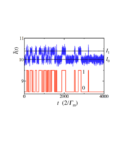
Figure 1: Numerical simulation of the selective evolution at $\delta V(0)=0.82$. Upper panel: the average current $\bar{I}(t)$; lower panel: the filtered data correponding to the states $|0\rangle$ and $|1\rangle$.

Starting from the initial state $|0\rangle$, the selective evolution is first simulated over a duration $2n_{p}/\Gamma_{m}$ with $n_{p}=2000$. For $\delta t\ll 1/\Gamma_{m}$, the measured current $I(t)$ contents a large fluctuation with $\sqrt{\langle\xi^{2}\rangle}\gg\Delta I$. We process the measurement record by averaging the current over an interval $2/\Gamma_{m}$: $\bar{I}(2n/\Gamma_{m})=\frac{\Gamma_{m}\delta t}{2}\sum I(t)$ for $2n/\Gamma_{m}\leq t<2(n+1)/\Gamma_{m}$. The average current $\bar{I}$ now contents a fluctuation smaller than $\Delta I$ and can be used to indicate the qubit states. In Fig.1, $\bar{I}$ is plotted versus time with $\bar{I}(0)\approx I_{0}$. During the evolution, the average current switches between $\bar{I}\approx I_{0}$ and $\bar{I}\approx I_{1}$ corresponding to switchings between the states $|0\rangle$ and $|1\rangle$. The number of switchings is determined by the rate $\tau_{jp}^{-1}$, from which we derive the first estimation of the noise magnitude $\delta V_{1}\approx|\delta V|$. To determine the sign of the noise, we shift the off-diagonal coupling in Eq. (1) by a constant $-\hbar\delta V_{1}/2$ and continue the simulation for another duration $2n_{p}/\Gamma_{m}$. For $\delta V>0$, the total off-diagonal coupling is decreased after the shift and subsequently the number of switchings is decreased in the second part of the simulation. For $\delta V<0$, the total off-diagonal coupling is increased after the shift and so does the number of switchings. After the evolution, we derive the second estimation of the noise magnitude $\delta V_{2}$. It can be shown that $\delta V_{2}=|\delta V|/2$ for $\delta V>0$ and $\delta V_{2}=3|\delta V|/2$ for $\delta V<0$. Finally, the noise is estimated as

$$\delta V_{c}=\{\begin{array}[]{cc}\frac{\delta V_{1}}{2}+\delta V_{2},&\textrm{for}\,\delta V_{1}>\delta V_{2}\\ -\frac{\delta V_{1}}{2}-\frac{\delta V_{2}}{3},&\textrm{for}\,\delta V_{1}<\delta V_{2}\end{array}$$

with both magnitude and sign. The parameters used in Fig.1 are $E_{z}=7$, $\Gamma_{m}=0.1$, $\delta V(0)=0.82$ at the start of the simulation, $\delta V(4n_{p}/\Gamma_{m})=0.87$ at the end of the simulation, $I_{0}=10$ and $I_{1}=10.4$ with the noise spectrum $S_{I}=0.4$. To count the number of switchings, the current $\bar{I}$ is filtered to be $0$ or $1$, which is also shown in Fig.1. In the first part of the simulation, the number of switchings is $n_{jp}^{(1)}=29$; in the second part, the number of switchings is $n_{jp}^{(2)}=7$. It is obvious from Fig. 1 that the switchings in the second part are much sparser than that in the first part. The estimated noise is $\delta V_{c}=0.73$. By shifting the off-diagonal coupling in Eq. (1) with the calibrated value $\delta V_{c}$, the dephasing can be reduced by a factor $\left|\frac{\delta V_{c}-\delta V(4n_{p}/\Gamma_{m})}{\delta V(0)}\right|^{4}\approx 10^{-3}$.

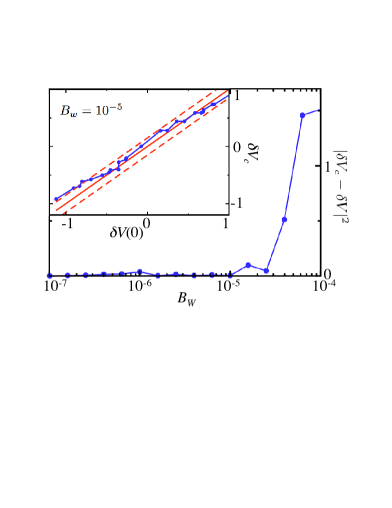
Figure 2: Main: residue noise $|\delta V_{c}-\delta V(4n_{p}/\Gamma_{m})|^{2}$ versus band width $B_{w}$. The solid circles connected by the solid curve are the residue noise from the simulation. Inset: $\delta V_{c}$ versus $\delta V(0)$ at $B_{w}=10^{-5}$. The solid circles connected by the solid curve are $\delta V_{c}$. The straight solid line in the middle is $\delta V(0)$ and the two dashes lines are $\delta V(0)\pm 0.15$.

The effectiveness of the above calibration depends sensitively on the band width of the low-frequency noise. In Fig.2, the average squared residue noise $\langle|\delta V_{c}-\delta V(4n_{p}/\Gamma_{m})|^{2}\rangle$ is plotted versus the band width $B_{w}$. For $B_{w}<(4n_{p}/\Gamma_{m})^{-1}$, the residue noise is much smaller than $\langle\delta V^{2}\rangle$. For $B_{w}\geq(4n_{p}/\Gamma_{m})^{-1}$, the residue noise increases dramatically. Thus, when the duration of the calibration is shorter than the time scale of the noise, the calibration is successful. With our parameters, $(4n_{p}/\Gamma_{m})^{-1}=1.3\cdot 10^{-5}$ agrees well with the sharp increase in the residue noise near this band width. In the inset of Fig.2, the calibrated value $\delta V_{c}$ is plotted versus the initial value of the noise at $B_{w}=10^{-5}$. It can be seen that the residue noise is mostly limited within $\pm 0.15$.

The residue noise of the calibration results from two factors: the finite accuracy due to finite number of switchings during the continuous measurement, and the time evolution of the low-frequency noise during the measurement. First, the probability of switching during a time $t$ is a Poissonian process with $p(t)=e^{-t/\tau_{jp}}$. For a duration $2n_{p}/\Gamma_{m}$, the average number of switchings is $\bar{n}_{jp}=2n_{p}/\Gamma_{m}\tau_{jp}$ with a deviation $\Delta n_{jp}=\sqrt{\bar{n}_{jp}}$. The finite accuracy can be derived as

$$\Delta V_{1}^{2}=\left|\frac{\partial\delta V}{\partial n_{jp}}\Delta n_{jp}\right|^{2}=\frac{4E_{z}^{2}+\Gamma_{m}^{2}}{8\Gamma_{m}T}$$ (6)

decreasing with the total measurement time $T$. Second, the variation of the noise due to time evolution is $\Delta V_{2}^{2}=\sum_{n}\frac{\beta}{\omega_{n}}\langle\alpha_{n}^{2}\rangle\langle\sin^{2}(\omega_{n}T+\varphi_{n})\rangle\omega_{n}^{2}T^{2}$ for $B_{w}T\ll 1$. With $\langle\alpha_{n}^{2}\rangle=1/3$ and $\langle\sin^{2}\varphi_{n}\rangle=1/2$, we derive

$$\Delta V_{2}^{2}=\frac{\beta}{12\Delta\omega}B_{w}^{2}T^{2}$$

increasing quadratically with $T$. Hence the residue noise $\Delta V_{c}^{2}=\Delta V_{1}^{2}+\Delta V_{2}^{2}$ can be minimized by varying the measurement time. With our parameters, the optimal time is $T\approx 1400/\Gamma_{m}$.

The calibration of the low-frequency noise can be exploited to improve the fidelity of quantum-logic gates. Let a qubit be encoded with two physical qubits, each of which is calibrated alternatively. The system is programed so that at any moment one of the two physical qubits has been calibrated and can be used for quantum memory or quantum-logic operations, while the other qubit is being calibrated. As an example, we consider a bit-flip gate on a single qubit encoded with physical qubits $q_{1}$ and $q_{2}$, as is shown in the box in Fig.3. First, a continuous measurement is performed on qubit $q_{1}$ for calibration. Afterward, the initial state is prepared in $q_{1}$ and the bit-flip gate is performed. At the same time, a continuous measurement is performed on qubit $q_{2}$. After this calibration, the state of $q_{1}$ is swapped to the calibrated $q_{2}$, which is followed by other gate operations on $q_{2}$. Below we assume that the off-diagonal coupling of our qubits can be tuned with large magnitude, while the eigenenergies are nearly fixed VionScience2002 . In this case, a Hadamard gate $\hat{U}_{h}=e^{-i(\sigma_{z}+\sigma_{x})\frac{\pi}{2\sqrt{2}}}$ can be performed by applying an off-diagonal coupling $\hbar E_{z}$; and a phase gate $\hat{U}_{ph}=e^{-i\sigma_{x}\frac{\pi}{2}}$ can be performed by applying zero off-diagonal coupling. The bit-flip gate is achieved with $\hat{U}_{flip}=\hat{U}_{h}\hat{U}_{ph}\hat{U}_{h}$. The low-frequency noise adds a small off-diagonal term to the Hamiltonian and affects the fidelity of the gates. The fidelity is defined as $F=|\langle\psi_{t}|\hat{U}|\psi_{i}\rangle|^{2}$ NielsenBook where $|\psi_{i}\rangle$ is the initial state, $|\psi_{t}\rangle$ is the target state by ideal quantum gates, and $\hat{U}$ is the gate operation with either the noise or the residue noise. In Fig.3, the fidelity of the bit-flip gate is plotted with the uncalibrated noise and the residue noise respectively. Without calibration, the fidelity decreases quadratically with the magnitude of the noise. The calibration can significantly improve the gate performance to have high fidelity in nearly all range of the noise. Note that this feature is universal for other single-qubit gates and two qubit gates.

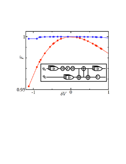
Figure 3: Fidelity of the bit-flip gate. The solid circles connected by the upper curve are the fidelity of the gate with the residue noise; the solid circles connected by the lower curve are the fidelity of the gate with the noise $\delta V(0)$. The box inside the plot: the time sequence of the calibrations and the gates.

This approach of reducing decoherence due to the low-frequency noise can be an important alternative to the dynamical control approach and quantum error correction approach FacchiPRA2005 . In a dynamical control approach, pulses much faster than $B_{w}^{-1}$ are applied all the time during the gate operations and the quantum memory period to cancel the effect of the noise ShiokawaPRA2004 ; GutmannPRA2005 ; FalciPRA2004 ; FaoroPRL2004 . Meanwhile, it is necessary to carefully engineer the pulses to avoid affecting the gate operations. In the quantum error correct approach, many ancilla qubits are required to correct the quantum errors NielsenBook ; Gottesman ; KnillNature2005 . While in our method, only a small number of physical qubits are needed to encode one qubit. Between the calibrations, no extra pulse or measurement is required.

To conclude, we showed that the low-frequency noise can be calibrated in the time-domain by a continuous measurement. Assisted by the continuous measurement, the off-diagonal coupling of the low-frequency noise induces second-order relaxation between the qubit states. We studied the stochastic evolution of the continuous measurement by numerical simulation and used the switchings between the qubit states to calibrate the noise. This approach can be a useful tool for suppressing decoherence due to the low-frequency noise in a solid-state qubit in addition to existing approaches. The next steps are to study the extension of this scheme to multiple qubits and to construct scalable quantum computing protocols based on the calibration scheme.

- (1) M. A. Nielsen and I. L. Chuang, Quantum Computation and Quantum Information (Cambridge University Press, Cambridge, 2000).
- (2) D. Gottesman, ‘Quantum Error Correction and Fault-Tolerance’, quant-ph/0507174.
- (3) E. Knill, Nature 434, 39 (2005).
- (4) M. B. Weissman, Rev. Mod. Phys. 60, 537 (1988).
- (5) R. W. Simmonds, K. M. Lang, D. A. Hite, S. Nam, D. P. Pappas, and J. M. Martinis, Phys. Rev. Lett. 93, 077003 (2004); J. M. Martinis, K.B. Cooper,R. McDermott, M. Steffen, M. Ansmann, K.D. Osborn, K. Cicak, S. Oh, D.P. Pappas, R.W. Simmonds, and C. C.Yu, Phys. Rev. Lett. 95, 210503 (2005).
- (6) F. C. Wellstood, C. Urbina, and John Clarke, Appl. Phys. Lett. 85, 5296 (2004).
- (7) D. J. Van Harlingen, T. L. Robertson, B. L. T. Plourde, P. A. Reichardt, T. A. Crane, and J. Clarke, Phys. Rev. B 70, 064517 (2004).
- (8) O. Astafiev, Y. A. Pashkin, Y. Nakamura, T. Yamamoto, and J. S. Tsai, Phys. Rev. Lett. 93, 267007 (2004); O. Astafiev, Yu. A. Pashkin, Y. Nakamura, T. Yamamoto, and J. S. Tsai, Phys. Rev. Lett. 96, 137001 (2006).
- (9) A. B. Zorin, F.-J. Ahlers, J. Niemeyer, T. Weimann, H. Wolf, V. A. Krupenin and S. V. Lotkhov, Phys. Rev. B 53, 13682 (1996).
- (10) D. J. Wineland et al., Phil. Trans. R. Soc. Lond A 361, 1349 (2003).
- (11) T. Itakura and Y. Tokura, Phys. Rev. B 67, 195320 (2003); Y. M. Galperin, B. L. Altshuler, and D. V. Shantsev, cond-mat/0312490; A. Shnirman, G. Schön, I. Martin, and Y. Makhlin, Phys.Rev. Lett. 94, 127002 (2005); G. Falci, A. D’Arrigo, A. Mastellone, and E. Paladino, Phys. Rev. Lett. 94, 167002 (2005); L. Faoro and L. B. Ioffe, Phys. Rev. Lett. 96, 047001(2006).
- (12) Y. Nakamura, Y. A. Pashkin, T. Yamamoto, and J. S. Tsai, Phys. Rev. Lett. 88, 047901 (2002).
- (13) E. Collin, G. Ithier, A. Aassime, P. Joyez, D. Vion, and D. Esteve, Phys. Rev. Lett. 93, 157005 (2004).
- (14) K. Shiokawa and D. A. Lidar, Phys. Rev. A 69, 030302(R) (2004).
- (15) H. Gutmann, F. K. Wilhelm, W. M. Kaminsky, and S. Lloyd, Phys. Rev. A 71, 020302 (R) (2005).
- (16) G. Falci, A. D’Arrigo, A. Mastellone, and E. Paladino, Phys. Rev. A 70, 040101 (R) (2004).
- (17) L. Faoro and L. Viola, Phys. Rev. Lett. 92, 117905 (2004).
- (18) D. Vion, A. Aassime, A. Cottet, P. Joyez, H. Pothier, C. Urbina, D. Esteve, M. H. Devoret, Science 296, 886 (2002).
- (19) Y. Makhlin and A. Shnirman, Phys. Rev. Lett. 92, 178301 (2004).
- (20) C. Gardiner and P. Zoller, Quantum Noise (Springer-Verlarg, Berlin, 2000).
- (21) C. M. Caves and G. J. Milburn, Phys. Rev. A 36, 5543 (1987).
- (22) H. M. Wiseman and G. J. Milburn, Phys. Rev. Lett. 70, 548 (1993).
- (23) A. C. Doherty and K. Jacobs, Phys. Rev. A 60, 2700 (1999); K. Jacobs and P. L. Knight, Phys. Rev. A 57, 2301 (1998).
- (24) O. Oreshkov and T. A. Brun, Phys. Rev. Lett. 95, 110409 (2005).
- (25) A. N. Korotkov, Phys. Rev. B 63, 115403 (2001); A. N. Korotkov and D. V. Averin, Phys. Rev. B 64, 165310 (2001); A. N. Korotkov, Phys. Rev. B 67, 235408 (2003).
- (26) S. A. Gurvitz, Phys. Rev. B 56, 15215 (1997); A. Shnirman and G. Schön, Phys. Rev. B 57, 15400 (1998); H.-S. Goan and G. J. Milburn, Phys. Rev. B 64, 235307 (2001); S. A. Gurvitz, L. Fedichkin, D. Mozyrsky, and G. P. Berman, Phys. Rev. Lett. 91, 066801 (2003); S. D. Barrett and T. M. Stace, Phys. Rev. Lett. 96, 017405 (2006).
- (27) K. Y. R. Billah and M. Shinozuka, Phys. Rev. A 42, 7492 (1990).
- (28) P. Facchi, S. Tasaki, S. Pascazio, H. Nakazato, A. Tokuse, and D. A. Lidar, Phys. Rev. A 71, 022302 (2005).