Coherent control of collective spontaneous emission in an extended atomic ensemble and quantum storage

Abstract

Coherent control of collective spontaneous emission in an extended atomic ensemble resonantly interacting with single-photon wave packets is analyzed. A scheme for coherent manipulation of collective atomic states is developed such that superradiant states of the atomic system can be converted into subradiant ones and vice versa. Possible applications of such a scheme for optical quantum state storage and single-photon wave packet shaping are discussed. It is shown that also in the absence of inhomogeneous broadening of the resonant line, single-photon wave packets with arbitrary pulse shape may be recorded as a subradiant state and reconstructed even although the duration of the wave packets is larger than the superradiant life-time. Specifically the applicability for storing time-bin qubits, which are used in quantum cryptography is analyzed.

I Introduction

Motivated by the development of modern quantum information science there is significant interest in investigating the interaction of nonclassical states of light with atomic ensembles. One active research area is the development of optical quantum memories. Such devices, which can store and reconstruct quantum states of light, form a basic ingredient for optical quantum computers, dealing either with discrete quantum variables (qubits) represented by single-photon two-mode states of the electromagnetic field or with continuous quantum variables represented by the quadrature amplitudes of the field (see reviews Kok et al. ; Braunstein and van Loock (2005) respectively). There are experimental demonstrations based on electromagnetically induced transparency Chaneliére et al. (2005) for the discrete variable approach and off-resonant interaction of light with spin polarized atomic ensembles Julsgaard et al. (2004) for the continuous variable case. The photon echo based quantum memory proposal has also attracted considerable attention Kessel’ and Moiseev (1993); Moiseev and Kröll (2001); Moiseev et al. (2003); Kraus et al. (2006); Nilsson and Kröll (2005). Another cause of the interest is the possibility of atomic ensemble state manipulation using atom-photon correlation (see review Lukin (2003)). The creation of a robust entanglement of atomic ensembles using Raman scattering may be especially important for applications involving long-distance quantum communication Duan et al. (2001). Finally, much effort has been directed toward implementation of controllable sources of nonclassical states of light such as photon-number or Fock states, which represent an essential resource for the practical implementation of many ideas from quantum information. These sources can also be constructed using quantum storage techniques in optically dense atomic media Eisaman et al. (2004).

The motivation of all these investigations is that photons can interact much more strongly with ensembles containing a large number of atoms than with individual atoms. In addition there can be a further collective enhancement taking place because the absorption, emission or coherent scattering processes employed in several of these implementation schemes involve collective atomic modes. On the other hand, whenever the number of atoms is large, the contribution from the collective spontaneous emission Dicke (1954); Gross and Haroche (1982); Benedict et al. (1996) to the evolution of an atomic-field system can also be considerable and may need to be taken into account. Therefore the investigation of this phenomenon in various situations when light interacts with atomic ensembles is of interest.

In this paper we investigate the possibilities of coherent control of collective spontaneous emission in an extended atomic ensemble interacting with a single-photon wave packet and vacuum modes of the electromagnetic field. Spontaneous emission is normally considered as a noise, which should be inhibited. Various schemes for inhibiting or reducing spontaneous emission noise for the single atom case have been proposed and investigated. For example in Agarwal et al. (2001) excitation by $2\pi$-pulses on an auxiliary transition is used to change the phase of the excited state wave function and in this way inhibit the spontaneous decay. In an atomic ensemble confined to a volume with dimensions small compared to the wavelength of the emitted radiation the problem is reduced to the creation of antisymmetric subradiant states Dicke (1954); Mandel and Wolf (1995); DeVoe and Brewer (1996), which are also interesting as they may be a basis for forming a decoherence free subspace Lidar and Whaley for the excited ensemble. In extended atomic systems, which is a much more frequent experimental situation, the collective spontaneous emission is characterized by a sharp directedness in space and occurs only in a small fraction of all radiation modes. Therefore it is possible to implement coherent control of collective atomic states using coherent excitation through other non-collective modes. Such a manipulation of collective states may be used for quantum memories in the regime of optical subradiance inhibiting the normal spontaneous decay, an idea which was briefly outlined in Kalachev and Samartsev (2005).

The paper is organized as follows. In Sec. II, we introduce a physical model of interaction between an extended many atom system and a single-photon wave packet and present an analytical description of the superradiant forward scattering. In Sec. III, we present a scheme for coherent manipulation of collective atomic states that can transform superradiant states into subradiant ones and vice versa. In Sec. IV, we discuss possible applications of such a scheme for the creation of optical quantum memory devices and controlled sources of non-classical light states. In Sec. V, we propose some specific experimental implementations that may be used to observe these effects and some possible methods for subradiant state preparation.

II Physical model

Consider a system of $N\gg 1$ identical two-level atoms, with positions $\bm{\mathrm{r}}_{j}$ ($j=1,\ldots,N$) and resonance frequency $\omega_{0}$, interacting among themselves and with the external world only through the electromagnetic field. Let us denote the ground and excited states of $j$th atom by $\lvert 0_{j}\rangle$ and $\lvert 1_{j}\rangle$. The Hamiltonian of the system, in the interaction picture and rotating-wave approximation, reads

$$H=\sum_{j,\bm{\mathrm{k}},s}\hbar g_{\bm{\mathrm{k}},s}^{\ast}b_{j}^{\dagger}a_{\bm{\mathrm{k}},s}{\,e}^{i\bm{\mathrm{k}}\cdot\bm{\mathrm{r}}_{j}}{\,e}^{i(\omega_{0}-\omega)t}+\text{H.c.}$$ (1)

Here

$$g_{\bm{\mathrm{k}},s}=\frac{i}{\hbar}\left(\frac{\hbar\omega}{2\varepsilon_{0}V}\right)^{1/2}(\bm{\mathrm{d}}\cdot\bm{\mathrm{\varepsilon}}_{\bm{\mathrm{k}},s})$$ (2)

is the atom-field coupling constant, $b_{j}=\lvert 0_{j}\rangle\langle 1_{j}\rvert$ is the atomic transition operator, $a_{\bm{\mathrm{k}},s}$ is the photon annihilation operator in the radiation field mode with the frequency $\omega=kc$ and polarization unit vector $\bm{\mathrm{\varepsilon}}_{\bm{\mathrm{k}},s}$ ($s=1,2$), $V$ is the quantization volume of the radiation field (we take $V$ much larger than the volume of the atomic system), $\bm{\mathrm{d}}$ is the dipole moment of the atomic transition. For the sake of simplicity we assume that the vectors $\bm{\mathrm{\varepsilon}}_{\bm{\mathrm{k}},s}$ and $\bm{\mathrm{d}}$ are real.

To describe the interaction of the field with the atoms we use the approach Bonifacio and Lugiato (1975); Banfi and Bonifacio (1975). First, it is convenient to assume that
(i) the atomic system has a shape of a parallelepiped with the dimensions $L_{\alpha}$, ($\alpha=x,y,z$) and the atoms are placed in a regular cubic lattice, so that $N=N_{x}N_{y}N_{z}$ and $d=L_{\alpha}N_{\alpha}^{-1}$ is the interatomic distance,
(ii) the dimensions $L_{\alpha}$ are much larger, but the interatomic distance $d$ is much smaller, than the wavelength $\lambda=2\pi c\omega_{0}^{-1}$ of the atomic transition,
(iii) the center of the system lies in the origin of the reference frame. Then we can define the following collective atomic operators:

$$R_{\bm{\mathrm{q}}}=\sum_{j=1}^{N}b_{j}{\,e}^{-i\bm{\mathrm{q}}\cdot\bm{\mathrm{r}}_{j}},$$ (3)

where ${q}_{\alpha}=2\pi n_{\alpha}L_{\alpha}^{-1}$, $n_{\alpha}=0,1,\ldots,N_{\alpha}-1$. Hamiltonian (1) can now be expressed in terms of the collective operators obtaining

$$H=\sum_{\bm{\mathrm{q}},\bm{\mathrm{k}},s}\hbar g_{\bm{\mathrm{k}},s}^{\ast}R^{{\dagger}}_{\bm{\mathrm{q}}}a_{\bm{\mathrm{k}},s}\phi^{\ast}(\bm{\mathrm{q}}-\bm{\mathrm{k}}){\,e}^{i(\omega_{0}-\omega)t}+\text{H.c.},$$ (4)

where $\phi(\bm{\mathrm{x}})={N}^{-1}\sum_{j}{\exp}(i\bm{\mathrm{x}}\cdot\bm{\mathrm{r}}_{j})$ is the diffraction function. The presence of this function in the Hamiltonian underlines the fact that each atomic mode $\bm{\mathrm{q}}$ is coupled only to modes $\bm{\mathrm{k}}$ lying in a diffraction angle around $\bm{\mathrm{q}}$ Bonifacio and Lugiato (1975).

We are interested in the interaction of the atomic system with a single-photon wave packet. Therefore we have the following general form of the state of the system at the initial time $t=0$

$$\lvert\psi(0)\rangle=\sum_{\bm{\mathrm{k}},s}f_{\bm{\mathrm{k}},s}(0)\lvert 0\rangle\lvert 1_{\bm{\mathrm{k}},s}\rangle+\sum_{\bm{\mathrm{q}}}c_{\bm{\mathrm{q}}}(0)\lvert 1_{\bm{\mathrm{q}}}\rangle\lvert\text{vac}\rangle$$ (5)

with normalization condition

$$\sum_{\bm{\mathrm{k}},s}|f_{\bm{\mathrm{k}},s}(t)|^{2}+\sum_{\bm{\mathrm{q}}}|c_{\bm{\mathrm{q}}}(t)|^{2}=1,$$ (6)

where $\lvert 0\rangle=\lvert 0_{1},0_{2},\ldots,0_{N}\rangle$ is the ground state of the atomic system, $\lvert\text{vac}\rangle$ is the vacuum state of the radiation field, $\lvert 1_{\bm{\mathrm{k}},s}\rangle=a^{\dagger}_{\bm{\mathrm{k}},s}\lvert\text{vac}\rangle$ and $\lvert 1_{\bm{\mathrm{q}}}\rangle={N}^{-1/2}R^{{\dagger}}_{\bm{\mathrm{q}}}\lvert 0\rangle$.

Now, we assume that
(iv) a single-photon wave packet propagates in the $z$-direction, the excitation volume may be approximated by a cylinder with the cross section $S$ and the length $L_{z}$, and the wave front of the packet is planar inside the excitation volume,
(v) the Fresnel number of the excitation volume $F=S(L_{z}\lambda)^{-1}\approx 1$, so that the collective interaction of the whole ensemble of atoms with the quantum field takes place only for longitudinal modes $\bm{\mathrm{q}}$,
(vi) the duration of the single-photon wave packet as well as that of collective spontaneous emission are much greater than cooperative time $\tau_{c}$ Arecchi and Courtens (1970), which in turn is much greater than the correlation time of the vacuum reservoir $\tau_{E}=L_{z}c^{-1}$ (Born-Markov condition). Here

$$\tau_{c}=\left(\frac{8\pi T_{1}SL}{3\lambda^{2}cN}\right)^{1/2},$$ (7)

where $T_{1}$ is the inverse of the Einstein $A$ coefficient. With these assumptions the interaction of the atomic system with the electromagnetic field may be described in a one-mode approximation with respect to the atomic system and a one-dimensional approximation with respect to the field. Substituting Eqs. (4) and (5) in the Schrödinger equation and omitting the index $\bm{\mathrm{q}}$ for the single atomic mode we obtain

$$\frac{\partial f_{\bm{\mathrm{k}},s}(t)}{\partial t} = -ig_{\bm{\mathrm{k}},s}\sqrt{N}\phi(\bm{\mathrm{q}}-\bm{\mathrm{k}})c(t){\,e}^{-i(\omega_{0}-\omega)t},$$ (8)

$$\frac{\partial c(t)}{\partial t} = -i\sqrt{N}$$ (9)

$$\times\sum_{\bm{\mathrm{k}},s}g^{\ast}_{\bm{\mathrm{k}},s}\phi^{\ast}(\bm{\mathrm{q}}-\bm{\mathrm{k}})f_{\bm{\mathrm{k}},s}(t){\,e}^{i(\omega_{0}-\omega)t}.$$

Now it is convenient to define a single-photon dimensionless photon density at the origin of the reference frame ($\bm{\mathrm{r}}=0$). For the incoming wave packet we have

$$F_{\text{in}}(t)=\left(\frac{L_{x}L_{y}L_{z}}{L^{3}}\right)^{1/2}\sum_{\bm{\mathrm{k}},s}f_{\bm{\mathrm{k}},s}(0){\,e}^{i(\omega_{0}-\omega)t},$$ (10)

and for the emitted radiation we have the analogous equation with $F_{\text{in}}(t)$ and $f_{\bm{\mathrm{k}},s}(0)$ replaced by $F(t)$ and $f_{\bm{\mathrm{k}},s}(t)$, respectively. Then the solution of Eqs. (8) and (9) may be written as (see Appendix A)

$$c(t) = c(0){\,e}^{-t/2\tau_{R}}$$ (11)

$$-\frac{1}{\sqrt{\tau_{R}\tau_{E}}}\int_{0}^{\infty}d\tau F_{\text{in}}(t-\tau){\,e}^{-\tau/2\tau_{R}},$$

$$F(t) = F_{\text{in}}(t)+\sqrt{\frac{\tau_{E}}{\tau_{R}}}c(t),$$ (12)

where $\tau_{R}$ is the superradiant life-time:

$$\frac{1}{\tau_{R}}=\frac{N\mu}{T_{1}},\quad\frac{1}{T_{1}}=\frac{1}{4\pi\varepsilon_{0}}\frac{4d^{2}\omega_{0}^{3}}{3\hbar c^{3}},$$ (13)

and $\mu=3\lambda^{2}(8\pi S)^{-1}$ is a geometrical factor, which is approximately equal to the ratio of the diffraction solid angle of collective emission to $4\pi$. If we consider the case when $c(0)=0$ and substitute Eq. (11) into (12), we obtain a solution for superradiant resonant forward scattering of photons, which is well known in the theory of propagation of coherent pulses through a resonant medium and especially in the coherent-path model of nuclear resonant scattering of $\gamma$ quanta Hoy (1997):

$$F(t)=F_{\text{in}}(t)-\frac{1}{\tau_{R}}\int_{0}^{\infty}d\tau F_{\text{in}}(t-\tau){\,e}^{-\tau/2\tau_{R}}.$$ (14)

Under the approximations mentioned earlier, Eq. (14) describes the simplest regime of superradiant forward scattering, when the incoming field is scattered only once. Considering resonant propagation, e.g. of small area pulses as in Crisp (1970), this corresponds to samples with $\alpha L$ not far above 1. It may be noted that the collective superradiant atomic state $\lvert 1_{\bm{\mathrm{q}}}\rangle$ is known in the theory of nuclear resonant scattering as a nuclear exciton (see, for example, Smirnov (1999); Odeurs and Hoy (2005) and references therein). The principal point here is the indistinguishability of atoms in a macroscopic sample with respect to photon absorption and emission into the longitudinal modes of the electromagnetic field, which leads to enhancement of atomic-field interaction and directedness of collective spontaneous emission Scully et al. (2006). Since the photon propagation time $\tau_{E}$ is much less than the cooperative time $\tau_{c}=\sqrt{\tau_{R}\tau_{E}}$, which in turn is much less than the duration of incoming and scattered photons, propagation effects may be neglected. In fact, from the view point of propagating fields, the sample looks like a scattering center, which is characterized by an enhanced cross-section of the resonant transition with respect to longitudinal modes. But the interaction of the atomic system with transverse modes of electromagnetic field is not collective and these modes do not see an enhanced cross section. This is of key importance for the preparation of subradiant states in an extended atomic system, which will be considered in the next section.

III Superradiant and subradiant states of an extended atomic ensemble

In his basic paper Dicke (1954) Dicke considered the two regimes of collective spontaneous emission of photons: superradiance and subradiance, which result from the constructive and destructive interference of atomic states, respectively. In the first case, a system of inverted atoms undergoes the spontaneous transition to the ground state for a time inversely proportional to the number of atoms, while in the second case the rate of collective spontaneous emission, on the contrary, decreases compared to the rate of spontaneous emission of single atoms. In the ideal case of a localized system confined to a volume with dimensions small compared to the wavelength of the emitted radiation, the rate of collective spontaneous emission of photons is equal to zero if the atoms are in an antisymmetric collective state. If an atomic system is extended, the rate of collective spontaneous emission can be suppressed only for a few collective modes. In particular, one-mode subradiance can be observed in samples having a shape of a cylinder with proportions defined by the Fresnel number $F\approx 1$. It is well known that such a one-mode model of collective spontaneous emission is equivalent to the Dicke model Bonifacio et al. (1971), except that the rate of spontaneous emission decreases by the geometrical factor $\mu$. If we redefine atomic states $\lvert 1_{j}\rangle$ multiplying them by phase a factor $\exp(i\bm{\mathrm{q}}\cdot\bm{\mathrm{r}}_{j})$ and denote a collective one-mode atomic state $\lvert n_{\bm{\mathrm{q}}}\rangle$ corresponding to the excitation of $n$ atoms as $\lvert n\rangle$, then

$$\lvert 1\rangle = \frac{1}{\sqrt{N}}R^{{\dagger}}\lvert 0\rangle=\frac{1}{\sqrt{N}}\sum_{i}\lvert 0,\ldots,1_{i},\ldots,0\rangle,$$ (15)

$$\lvert 2\rangle = \frac{1}{\sqrt{2N(N-1)}}(R^{{\dagger}})^{2}\lvert 0\rangle$$ (16)

$$= \sqrt{\frac{2}{N(N-1)}}\sum_{j>i}\lvert 0,\ldots,1_{i},\ldots,1_{j},\ldots,0\rangle,$$

etc., where $R=\sum_{j=1}^{N}b_{j}$. The rate of collective spontaneous emission of photons ${\mu}{T_{1}}^{-1}|\langle n-1\rvert R\lvert n\rangle|^{2}$ is increased during excitation of the medium (for $n<\frac{N}{2}$). The spontaneous emission of a photon from the state $\lvert 1\rangle$ occurs with the rate $N\mu T_{1}^{-1}$ (see Eq. (13)), from the state $\lvert 2\rangle$ with the rate $2(N-1)\mu T_{1}^{-1}$, etc.

We assume now that atoms have the additional level $\lvert 2_{j}\rangle$ and the transition frequency $\omega_{12}$ differs from $\omega_{01}$ (Fig. 1). Then, irradiation by a short coherent $2\pi$ pulse at the frequency $\omega_{12}$ can almost instantly change the phase of the states $\lvert 1_{j}\rangle$, thereby changing the phase of the collective state $\lvert 1\rangle$ to the opposite one, while the phase of the state $\lvert 2\rangle$ remains unchanged.

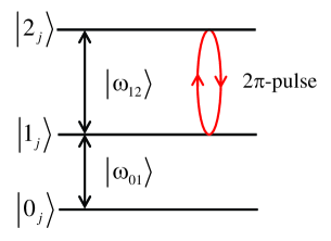
Figure 1: (Color online) Scheme of the working atomic levels, which are used for preparing subradiant collective states.

Let us divide a sample into two parts, $A$ and $B$, each containing $\frac{N}{2}$ atoms. It is convenient to represent superradiant states (15) and (16) in the form

$$\lvert 1_{A+B}\rangle = \frac{1}{\sqrt{2}}\big{(}\lvert 1_{A},0_{B}\rangle+\lvert 0_{A},1_{B}\rangle\big{)},$$ (17)

$$\lvert 2_{A+B}\rangle = \frac{1}{2\sqrt{N-1}}[\sqrt{N-2}(\lvert 2_{A},0_{B}\rangle+\lvert 0_{A},2_{B}\rangle)$$ (18)

$$+\sqrt{2N}\lvert 1_{A},1_{B}\rangle].$$

Upon irradiation of atoms in, for example, part B, by a coherent $2\pi$-pulse the atomic system passes from states (17) and (18) to the antisymmetric single-mode subradiant states

$$\lvert 1_{A-B}\rangle = \frac{1}{\sqrt{2}}(\lvert 1_{A},0_{B}\rangle-\lvert 0_{A},1_{B}\rangle),$$ (19)

$$\lvert 2_{A-B}\rangle = \frac{1}{2\sqrt{N-1}}[\sqrt{N-2}(\lvert 2_{A},0_{B}\rangle+\lvert 0_{A},2_{B}\rangle)$$ (20)

$$-\sqrt{2N}\lvert 1_{A},1_{B}\rangle].$$

The rate of photon emission from state (19) is identically zero, while that from state (20) is $2(N-1)^{-1}\mu T_{1}^{-1}$, i.e., goes to zero for large $N$.

Now assume that the atomic system in state (19) absorbs a photon and passes to the state

$$\lvert 2^{\prime}_{A-B}\rangle=\frac{1}{\sqrt{2}}(\lvert 2_{A},0_{B}\rangle-\lvert 0_{A},2_{B}\rangle).$$ (21)

The rate of photon emission in this case is $(N-2)\mu T_{1}^{-1}$, i.e., in fact essentially the same as the superradiant spontaneous decay from the state $\lvert 1\rangle$ at large $N$. To convert the state in Eq. (21) into a subradiant state, it is necessary to irradiate half of the atoms, whose phase was changed after absorption of the first photon, and half atoms, whose phase was not changed, by additional $2\pi$-pulses. As a result, the atomic system will be divided into four parts, which we denote $A$, $B$, $C$, and $D$, and the state of the system will take the form

$$\lvert 2_{A-B+C-D}\rangle=\frac{1}{\sqrt{2}}(\lvert 2_{A-B},0_{C+D}\rangle-\lvert 0_{A+B},2_{C-D}\rangle).$$ (22)

The rate of collective spontaneous emission from this state is equal to $4(N-2)^{-1}\mu T_{1}^{-1}$.

Therefore, by irradiating the system of atoms by $2\pi$ pulses through auxiliary transition after each absorption of a photon, we can transfer it into the next higher excited subradiant state, where the spontaneous transition from this state to the previous subradiant state will be forbidden. When transfering the atomic system into subradiant states repeatedly the action of the $2\pi$ pulses can be described using Hadamard matrixes

$$H_{2}=\left[\begin{array}[]{cc}1&1\\ 1&-1\\ \end{array}\right],\quad H_{2k}=\left[\begin{array}[]{cc}H_{k}&H_{k}\\ H_{k}&-H_{k}\\ \end{array}\right],$$ (23)

where $k=2,4,8,$ etc. The scheme for the preparation of different subradiant states can be seen directly from the matrix where each column correspond to one specific spatial part and, with the exception of the first row, each row shows the phase of all the spatial parts for a specific subradiant state. Transformation from one row to another is accomplished by phase shift $\lvert 1_{j}\rangle\to-\lvert 1_{j}\rangle$ for half of the atoms. The size $2k$ is equal to the number of the spatial parts and the total number of orthogonal subradiant states which can be prepare in such a way is $2k-1$.

IV Quantum memory applications and single-photon pulse shaping

Now, consider the writing and reading of a single-photon wave packet with a duration $T$ satisfying the condition $\tau_{R}\ll T$. The writing process will be divided into several time intervals, the duration of which is of the order of $\tau_{R}$ and much less than that of the single-photon wave packet $T$. Between the intervals, the atomic system is subjected to $2\pi$ pulses, which transfer it to different subradiant states. The duration of these pulses $t_{p}$ should be short in comparison with $\tau_{R}$. The probability of the failure of such a transformation is (see Appendix B)

$$p_{\text{failure}}=|c_{0}|^{2}\left(\frac{g_{a}\Omega_{R}}{g_{a}^{2}+(\Omega_{R}/2)^{2}}\right)^{2},$$ (24)

where $|c_{0}|^{2}$ is the probability that the atomic system is in the ground state and the field in a single-photon state, at the beginning of the transformation, $\Omega_{R}$ is the Rabi frequency of the coherent pulse and $g_{a}$ is the atom-field coupling constant on the transition $\lvert 0_{j}\rangle-\lvert 1_{j}\rangle$. Therefore if $\Omega_{R}\gg g_{a}$, $p_{\text{failure}}$ becomes close to 0.

The probability amplitude of photon absorption in each time interval is proportional to the wave-function amplitude of the photon in accordance with Eq. (11). Therefore, at the end of the writing process, the state of the atomic system will be determined by a superposition of orthogonal subradiant states, each corresponding to that the photon was absorbed in the corresponding time interval with a weight proportional to the single photon wave-function amplitude. If now the atomic system is subjected to a sequence of $2\pi$ pulses, which convert it back from the subradiant states to the superradiant states, the single-photon wave packet will be reconstructed, since the probability amplitude of a spontaneous photon emission is proportional to the amplitude of the excited atomic state at the start of the corresponding time intervals in accordance with Eq. (12). The simple example of single-photon writing and reconstruction is shown in Fig. 2.

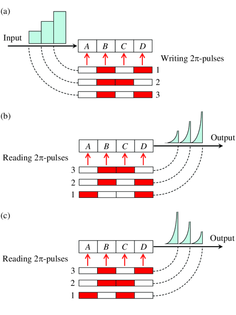
Figure 2: (Color online) Geometry and the temporal order of the action of $2\pi$-pulses preparing the subradiant states of an extended medium in the case of four spatial parts and three possible subradiant states. A filled area indicates the action of a $2\pi$-pulse in the corresponding spatial domain: (a) upon writing the quantum state of the single-photon wave packet, (b) upon read-out without time reversal, and (c) upon read-out with time reversal.

In this case the atomic system is divided into four spatial parts so that the preparation of three orthogonal subradiant states is possible, which corresponds to the following Hadamard matrix

$$H_{4}=\left(\begin{array}[]{cccc}1&1&1&1\\ 1&-1&1&-1\\ 1&1&-1&-1\\ 1&-1&-1&1\\ \end{array}\right).$$ (25)

Let $c_{n}$ be the probability amplitude that a photon has been captured during the $n$-th time interval. It is convenient to write the photon state in the following form

$$\lvert F\rangle=\sum_{n}f_{n}\lvert 1_{n}\rangle,$$

where $\lvert 1_{n}\rangle$ is an elementary single-photon wave packet propagating through the sample during the $n$-th time interval and $f_{n}$ is the probability amplitude to find a photon in the state $\lvert 1_{n}\rangle$. $\sum_{n}|c_{n}|^{2}=1$ and in the ideal case $c_{n}=f_{n}$ (within a phase factor insensitive to $n$). Then the evolution of the atomic-field system during the application of $2\pi$-pulses in accordance with the scheme (25) may be described as follows

$$\lvert 0\rangle(f_{1}\lvert 1_{1}\rangle+f_{2}\lvert 1_{2}\rangle+f_{3}\lvert 1_{3}\rangle)\to\\ c_{1}\lvert 1_{A-B+C-D}\rangle\lvert\text{vac}\rangle+\lvert 0\rangle(f_{2}\lvert 1_{2}\rangle+f_{3}\lvert 1_{3}\rangle)\to(c_{1}\lvert 1_{A+B-C-D}\rangle+c_{2}\lvert 1_{A-B-C+D}\rangle)\lvert\text{vac}\rangle+\lvert 0\rangle f_{3}\lvert 1_{3}\rangle\to\\ (c_{1}\lvert 1_{A-B-C+D}\rangle+c_{2}\lvert 1_{A+B-C-D}\rangle+c_{3}\lvert 1_{A-B+C-D}\rangle)\lvert\text{vac}\rangle.$$

The first pulse acts on parts $BD$, the second on $BC$, and the third on $BD$ again [Fig. 2(a)]. Now the shape of a single-photon wave packet is stored as the set of amplitudes $c_{n}$. In order to reconstruct the single-photon state we apply three $2\pi$-pulses, which act on parts $AD$, $BD$, and $BC$, respectively [Fig. 2(b)]. It should be noted that after the action of the first read-out pulse the phase of the emitted wave-packet becomes the same as for the incoming one. Let $e_{n}$ be the probability amplitude that the photon has been emitted between the application of the $n$-th and $(n+1)$-th read-out pulses. Then the evolution of the atomic-field system upon the reading of information reads

$$(c_{1}\lvert 1_{A-B-C+D}\rangle+c_{2}\lvert 1_{A+B-C-D}\rangle+c_{3}\lvert 1_{A-B+C-D}\rangle)\lvert\text{vac}\rangle\to\\ \lvert 0\rangle e_{1}\lvert 1_{1}\rangle+(c_{2}\lvert 1_{-A+B-C+D}\rangle+c_{3}\lvert 1_{-A-B+C+D}\rangle)\lvert\text{vac}\rangle\to\lvert 0\rangle(e_{1}\lvert 1_{1}\rangle+e_{2}\lvert 1_{2}\rangle)+c_{3}\lvert 1_{-A+B+C-D}\rangle\lvert\text{vac}\rangle\to\\ \lvert 0\rangle(e_{1}\lvert 1_{1}\rangle+e_{2}\lvert 1_{2}\rangle+e_{3}\lvert 1_{3}\rangle),$$

where $e_{n}=f_{n}$ in the ideal case. Moreover, by rearranging the coherent $2\pi$ pulses at the reading stage, we can permute the superradiant states and form a preassigned shape of the emitted single-photon wave packet. For example, the application of reading $2\pi$ pulses to the parts $AC$, $BC$ and $BD$ leads to the reversal of a single photon wave packet [see Fig. 2(c)]. Besides, it is possible to modulate the phase of the emitted photon at each elementary act of read-out by applying $2\pi$-pulses to spatial regions, which are complimentary to those used for the writing.

The number of subradiant states used for the storage of a single photon wave packet determines the time resolution of the quantum memory. The reconstructed pulse shape in general case is different from the original one, but the probability distribution within the time intervals between $2\pi$-pulses is the same. Therefore, such a quantum memory may be useful, for example, for a quantum communication using time-bin qubits or, more generally, time-bin qudits. The procedure described here for the case of a single photon may be extended in a straightforward way in order to write and reconstruct a sequence of photons. In this case it is necessary to increase the total number of orthogonal subradiant states and corresponding number of spatial parts as was described in Sec. III. By rearranging the read-out pulses we can form not only a preassigned shape of the emitted single-photon wave packets, but also a preassigned sequence of them.

In order to estimate the efficiency of the writing and reading processes consider the solution (11) for the case when all atoms are in the ground state at time $t=0$ and the single-photon wave packet has a quasi-rectangular form with a duration $\tau_{\text{ph}}$ and amplitude $F_{\text{in}}(t)=\sqrt{\tau_{E}/\tau_{\text{ph}}}$. The term ’quasi-rectangular form’ means that the leading and trailing fronts of the pulse are not shorter than $\tau_{E}$. (If this would not be the case the one-mode approximation becomes invalid.) Then from Eq. (11) we obtain

$$c(t)=\left\{\begin{array}[]{ll}2\sqrt{\dfrac{\tau_{R}}{\tau_{\text{ph}}}}\left[\exp\left(-\dfrac{t}{2\tau_{R}}\right)-1\right],&\text{$t\leq\tau_{\text{ph}}$,}\\ c(\tau_{\text{ph}})\exp\left(-\dfrac{t-\tau_{\text{ph}}}{2\tau_{R}}\right),&\text{$t>\tau_{\text{ph}}$.}\\ \end{array}\right.$$ (26)

The maximum of $|c(t)|$ is equal to 0.9 and is attained when $\tau_{\text{ph}}\approx 2.5\tau_{R}$. The population of the excited atomic state $|c(t)|^{2}$ as a function of time for the case when the incoming wave packet has a rectangular shape is shown in Fig. 3.

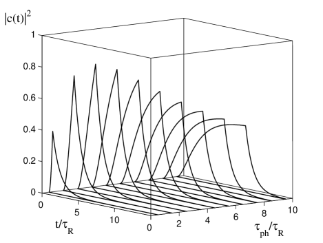
Figure 3: The population of the excited atomic state $|c(t)|^{2}$ as a function of time $t$ and duration of rectangular incoming wave packet $\tau_{ph}$.

Thus, the efficiency of the writing process for a wave packet of duration $T\gg\tau_{R}$ is equal to 81% when the $2\pi$-pulses separated by $2.5\tau_{R}$, which is the optimal value. Since the duration of the elementary read-out act is also equal to $2.5\tau_{R}$, the efficiency of read-out of information is equal to $1-\exp(-2.5)$, i.e., 91%. Therefore the total efficiency of the scheme proves to be about 75%. It is also possible to find pulse shapes that will enable storage and recall with a similar overall efficiency of 75% in a self-consistent regime, where the output pulse has the same shape as the input pulse.

However, if each pulse only need to be stored and read once the memory can be operated in a nearly 100% efficient mode. In accordance with Eq. (11) the probability of absorption is maximal for a propagating pulse like

$$F_{\text{in}}(t)=\left\{\begin{array}[]{ll}\sqrt{\dfrac{\tau_{E}}{\tau_{R}}}\exp\left(\dfrac{t-t_{\text{end}}}{2\tau_{R}}\right),&\text{$t\leq t_{\text{end}}$,}\\ 0,&\text{$t>t_{\text{end}}$,}\\ \end{array}\right.$$ (27)

where $t_{\text{end}}\gg\tau_{R}$. In this case we have

$$c(t)=\left\{\begin{array}[]{ll}-\exp\left(\dfrac{t-t_{\text{end}}}{2\tau_{R}}\right),&\text{$t\leq t_{\text{end}}$,}\\ -\exp\left(-\dfrac{t-t_{\text{end}}}{2\tau_{R}}\right),&\text{$t>t_{\text{end}}$.}\\ \end{array}\right.$$ (28)

Therefore, $|c(t)|^{2}=1$ at the end of the pulse $t=t_{\text{end}}$. Now, if we apply a $2\pi$-pulse to half the atoms at this time, a subradiant state is created with unit probability. Upon read-out we obtain (with unit probability) the pulse shape

$$F(t)=\sqrt{\frac{\tau_{E}}{\tau_{R}}}\exp\left(-\frac{t-t_{\text{read}}}{2\tau_{R}}\right),\quad t\geq t_{\text{read}},$$ (29)

corresponding to spontaneous emission after the application of a short read-out pulse at the time $t=t_{\text{read}}$ (the phase of the emitted photon can be changed by $\pi$ at the read-out as was considered above). Thus, nearly unit efficiency quantum storage with time reversal is possible for wave-packets of the form in Eq. (27). Such a regime may be useful, for example, for a long-distance quantum communication using quantum repeaters Briegel et al. (1998), when the qubits are only stored and recalled once before being measured. Assuming that faint laser pulses are used for carrying the information Gisin et al. (2002), the preparation of a time-bin qubit, which is a superposition of well separated exponential wave packets like (27), is not a challenging experimental task. Each of the wave-packets may be recorded (reconstructed) using only one transformation to (from) a subradiant state.

In conclusion of this section, it should be noted that the simple model of quantum storage with time reversal may be generalized to include propagation effects. In this case the shape of pulses to be stored should be determined by the time-reversed response function of a sample. As a result, both recorded and reconstructed wave-packets prove to be modulated in time, but the unit efficiency of quantum storage is maintained.

V Implementing the scheme in a solid state medium

Solids and especially rare-earth-ion-doped crystals are attractive materials for optical and quantum optical memories. At cryogenic temperatures optical transitions of rare-earth-ion-doped crystals have very narrow homogeneous lines, which correspond to long phase relaxation of the optical transitions, up to milliseconds Macfarlane (2002). But observation of collective spontaneous emission in solids as well as related effects such as superradiant forward scattering considered above is a nontrivial experimental problem. Since inhomogeneous broadening of optical transitions is usually several GHz and oscillator strengths are small, it is in order to fulfill the condition $\tau_{R}\ll T_{2}^{\ast}$, necessary to use very high densities of impurities and perform observations in the ps regime or to use frequency selective excitation of the inhomogeneous profile, which significantly limits the superradiant effect. From this point the technique of preparing of narrow absorbing peaks on a non-absorbing background, i.e. isolated spectral features corresponding to a group of ions absorbing at a specific frequency, in rare-earth-ion-doped crystals Pryde et al. (2000); Sellars et al. (2000); Nilsson et al. (2002); de Sèze et al. (2003); Nilsson et al. (2004); Rippe et al. (2005) can be very useful. Such specific structures can be created as follows. First, spectral pits, i.e. wide frequency intervals within the inhomogeneous absorption profile that are completely empty of all absorption, are created using hole-burning techniques. The maximum width of the pits is determined by the hyperfine level separations Nilsson et al. (2004). Then narrow peaks of absorption can be created by pumping ions absorbing within a narrow spectral interval back into the emptied region. It is possible to select only a subset of ions absorbing on a transition between specific hyperfine levels in the ground and excited states Nilsson et al. (2004). The peaks can have a width of the order of the homogeneous linewidth, if a laser with a sufficiently narrow linewidth is used for the preparation.

We now turn to a specific example of how to realize quantum state storage under the optical subradiance regime, using the ${}^{3}H_{4}(1)-{}^{1}D_{2}(1)$ transition of $\text{Pr}^{3+}$ ions in $\text{Y}_{2}\text{SiO}_{5}$. The optical properties of this crystal has been studied extensively and the preparation of narrow absorption peaks have already been demonstrated on this transition in experiments mentioned above. The ground state is split into three doubly degenerate states, which are usually labeled $\lvert\pm 1/2\rangle$, $\lvert\pm 3/2\rangle$, and $\lvert\pm 5/2\rangle$, separated by 10.2 and 17.3 MHz Holliday et al. (1993); Equall et al. (1995) for ions in site 1. A narrow absorption peak with a line-width of less than $\Gamma_{\text{inh}}=100$ kHz is usually created in one of these states on a $10-15$ MHz wide pit in the absorption profile. The life-time of the excited optical state $T_{1}=164\;\mu\text{s}$ and the homogeneous line-width is 2.4 kHz. These values correspond to crystals at liquid helium temperature. The total inhomogeneous broadening of the optical transition is of the order of 4 GHz, so that the Pr ion density within a 100 kHz frequency interval is roughly equal to $2\times 10^{20}\;\text{m}^{-3}$ for crystals with Pr doping concentration of 0.05% ($9\times 10^{24}\;\text{m}^{-3}$). The principal point here is the possibility of changing this density from that maximum value down to zero when preparing the narrow absorption peaks. This can be a convenient way to investigate a transition from incoherent spontaneous emission to superradiance in a given crystal by adjusting the superradiant life-time $\tau_{R}$ to the desirable value. Taking the wavelength of the optical transition $\lambda=606$ nm, the length of a sample $L_{z}=5$ mm, the diameter of a focal spot $100\;\mu\text{m}$, we obtain $\tau_{E}=17$ ps, $\mu=0.5\times 10^{-5}$ and $\tau_{R}=3.7$ ns. The last value is too short because the pit width is equal to 10 MHz so that the duration of superradiant decay should be longer than 20 ns. If we decrease the ion density down to $2\times 10^{19}\;\text{m}^{-3}$, we obtain obviously $\tau_{R}=37$ ns, which may be considered as the shortest possible value. On the other hand, the upper limit for the superradiant decay time is given by the inhomogeneous life-time $T_{2}^{\ast}=(\pi\Gamma_{\text{inh}})^{-1}$, which in this case is equal $3\;\mu\text{s}$. With the parameters mentioned above we obtain $\tau_{R}=1.9\;\mu\text{s}$ for an ion density of $4\times 10^{17}\;\text{m}^{-3}$, which may be considered as a lower bound. Thus, we can conclude that the observation of optical superradiance in the time scale $10^{2}-10^{3}$ ns is possible. It should be noted that by decreasing the inhomogeneous broadening of the absorption peak down to 10 kHz we obtain an inhomogeneous life-time of $T_{2}^{\ast}=30\;\mu\text{s}$. Therefore, in principle, it is possible to make $\tau_{R}$ of the order of several microseconds, which may be very useful for initial investigations of subradiant states in such a system. Since dipole moments of optical transitions are rather small (for example, 0.0078 D for the transition ${}^{3}H_{4}(1)-{}^{1}D_{2}(1)$ Nilsson et al. (2004)), such values of $\tau_{R}$ allow the use of $2\pi$-pulses with a duration up to $100-200$ ns, thereby reducing the intensity of excitation pulses.

V.1 Active preparation of subradiant states

The active preparation implies that the phases of atomic states are modulated by excitation pulses, such as the $2\pi$-pulses considered above. A scheme for preparing orthogonal subradiant states that may be simpler from an experimental point of view is shown in Fig. 4(a). In this case two non-collinear $\pi$-pulses are applied in sequence instead of a single $2\pi$-pulse. Suppose that $\bm{\mathrm{k}}_{1}$ and $\bm{\mathrm{k}}_{2}$ are wave vectors of the first and second pulses, respectively, in a pair and the vector $\bm{\mathrm{k}}_{1}-\bm{\mathrm{k}}_{2}$ is directed along the sample $z$ axis. After the excitation the collective atomic state $\lvert 1_{\bm{\mathrm{q}}}\rangle$ becomes $-\lvert 1_{\bm{\mathrm{q}}+\bm{\mathrm{k}}_{1}-\bm{\mathrm{k}}_{2}}\rangle$. It follows that such an excitation leads to an added phase shift while propagating through the medium. If this phase shift is a multiple of $2\pi$, i.e. $|\bm{\mathrm{k}}_{1}-\bm{\mathrm{k}}_{2}|=2\pi mL_{z}^{-1}$, where $m$ is an integer, a subradiant state is obtained. The rate of collective spontaneous emission into the longitudinal mode proves to be zero due to destructive interference between various spatial parts. (We propose here that $m$ is small, i.e. $|\bm{\mathrm{k}}_{1}-\bm{\mathrm{k}}_{2}|\ll\omega_{0}/c$.) Different values of $m$ correspond to different orthogonal subradiant states. In order to convert the system back from the subradiant state into the superradiant state the same pulses need to be applied in reverse order, i.e. the wave vectors of the first and second read-out pulses should be $\bm{\mathrm{k}}_{2}$ and $\bm{\mathrm{k}}_{1}$ respectively.

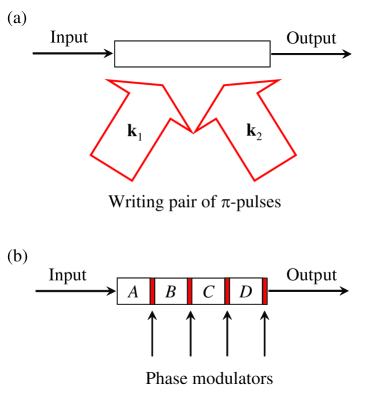
Figure 4: (Color online) Scheme for the preparation of subradiant states in an extended atomic ensemble using (a) pairs of non-collinear and non-simultaneous coherent $\pi$-pulses and (b) controllable bi-phase modulators in the case of four spatial parts.

Compared to the excitation by $2\pi$-pulses the advantage of such an excitation is that the second $\pi$-pulse in a pair can transfer an atomic state from the excited level to another long-lived ground level. In this case the storage time may be much longer than the life-time of the excited states.

V.2 Passive preparation of subradiant states

On the other hand, it is not necessary to create a phase shift using coherent excitation pulses. We can create it by controllable phase modulators inserted into the atomic ensemble as shown in Fig. 4(b). Suppose that each of the modulators may be in one of two possible states: an off-state, when it does not create a phase shift, and an on-state, when a $\pi$ phase shift is created. Now, we turn on and turn off these bi-phase modulators in a definite order instead of application of $2\pi$-pulses. A subradiant state is obtained if destructive interference of radiation emitted from various spatial parts occurs at the exit of the sample and, of course, if the emission process remains collective for the whole system. In the case of four spatial parts, if we want to obtain the sequence of subradiant states which corresponds to the Hadamard matrix (25), we should switch the phase modulators in the following order: $ABCD\to\bar{A}B\bar{C}D\to A\bar{B}C\bar{D}$, where $A$ ($\bar{A}$) means that the modulator after the part $A$ is turned on (turned off) and so on. The read out without time reversal is described by the following scheme: $\bar{A}\bar{B}\bar{C}{D}\to ABC\bar{D}\to\bar{A}{B}\bar{C}\bar{D}$.

Compared to the active preparation scheme such a passive preparation scheme may have several advantages. Single-photon wave packets propagating in optical fibers or wave guides can be stored and reconstructed without using transverse coherent excitation. The only condition is that photon propagation time through the whole system should be shorter than $\tau_{R}$. Further, an atomic ensemble (or each optical center) may be placed in a confined space or artificial structure like a photonic crystal such that spontaneous emission into transverse modes is inhibited. In this case controlling the emission and creating subradiant states for the longitudinal modes may enable storage of qubit states in decoherence free substates in the ensemble during times which may be longer than the excited state life-time of a free atom.

VI Conclusion

It is shown that single-photon wave packets with arbitrary pulse shape resonant with a transition in an ensemble of atoms may be recorded and reconstructed in a regime of optical subradiance also in the absence of inhomogeneous broadening of the resonant transition. Homogeneously broadened lines are more prone to superradiance than inhomogeneously broadened lines but the technique described here allows the writing and reconstruction of time-bin qubits in an optically dense medium also when the time-bin qubit duration exceeds the superradiant life-time for the ensemble. This approach could therefore open a new window in the search of materials for quantum memories.

Appendix A

To solve the equations (8) and (9) we use the Laplace transformation

$$\bar{y}(z) =\int_{0}^{\infty}e^{-zt}y(t)\,dt,$$ (30)

$$z\bar{y}(z)-y(0) =\int_{0}^{\infty}e^{-zt}\dot{y}(t)\,dt$$ (31)

and obtain

$$z\bar{f}_{\bm{\mathrm{k}},s}(z)-f_{\bm{\mathrm{k}},s}(0) = -ig_{\bm{\mathrm{k}},s}\sqrt{N}\phi(\bm{\mathrm{q}}-\bm{\mathrm{k}})$$ (32)

$$\times\bar{c}(z+i(\omega_{0}-\omega)),$$

$$z\bar{c}(z)-c(0) = -i\sum_{\bm{\mathrm{k}},s}g_{\bm{\mathrm{k}},s}^{\ast}\sqrt{N}\phi^{\ast}(\bm{\mathrm{q}}-\bm{\mathrm{k}})$$ (33)

$$\times\bar{f}_{\bm{\mathrm{k}},s}(z-i(\omega_{0}-\omega)).$$

For the atomic excitation amplitude we find

$$\bar{c}(z)=\frac{c(0)-i\sum_{\bm{\mathrm{k}},s}\dfrac{g_{\bm{\mathrm{k}},s}^{\ast}\sqrt{N}\phi^{\ast}(\bm{\mathrm{q}}-\bm{\mathrm{k}})f_{\bm{\mathrm{k}},s}(0)}{z-i(\omega_{0}-\omega)}}{z+\sum_{\bm{\mathrm{k}},s}\dfrac{|g_{\bm{\mathrm{k}},s}|^{2}N|\phi(\bm{\mathrm{q}}-\bm{\mathrm{k}})|^{2}}{z-i(\omega_{0}-\omega)}}.$$ (34)

In the Born-Markov approximation we can evaluate the sum in the denominator by first converting it to an integral

$$\sum_{\bm{\mathrm{k}}}\to\frac{L^{3}}{(2\pi)^{3}c^{3}}\sum_{0}^{\infty}\omega^{2}\,d\omega\int d\Omega_{\bm{\mathrm{k}}}$$ (35)

and then employing the identity

$$\lim_{z\to 0}\frac{1}{z-i(\omega_{0}-\omega)}=\pi\,\delta(\omega_{0}-\omega)+i\frac{P}{\omega_{0}-\omega}$$

with $P$ denoting the principal value. As a result we obtain

$$\sum_{\bm{\mathrm{k}},s}\frac{|g_{\bm{\mathrm{k}},s}|^{2}N|\phi(\bm{\mathrm{q}}-\bm{\mathrm{k}})|^{2}}{z-i(\omega_{0}-\omega)}=\Gamma+i\Delta,$$ (36)

where

$$\Gamma=\frac{d^{2}N\mu\omega_{0}^{3}}{6\pi\hbar\varepsilon_{0}c^{3}}$$

is the collective atomic linewidth and $\Delta$ is the collective frequency shift, which may be neglected. Here $\mu=3\lambda^{2}(8\pi S)^{-1}$ is a geometrical factor Rehler and Eberly (1971), which describes the result of the integration

$$\int d\Omega_{\bm{\mathrm{k}}}\sum_{s}(\bm{\mathrm{d}}\cdot\bm{\mathrm{\varepsilon}}_{\bm{\mathrm{k}},s})^{2}\phi^{2}(\bm{\mathrm{q}}-\bm{\mathrm{k}})=\frac{8\pi}{3}\mu d^{2}$$ (37)

for a pencil-shaped cylindrical volume with the cross-section $S$, a vector $\bm{\mathrm{q}}$ lying along the axis of the cylinder and dipole moments oriented perpendicular to the axis. With the help of (36) the inverse Laplace transformation yields

$$c(t)=c(0){\,e}^{-\Gamma t} - i\sum_{\bm{\mathrm{k}},s}\frac{g_{\bm{\mathrm{k}},s}^{\ast}\sqrt{N}\phi^{\ast}(\bm{\mathrm{q}}-\bm{\mathrm{k}})f_{\bm{\mathrm{k}},s}(0)}{\Gamma+i(\omega_{0}-\omega)}$$ (38)

$$\times\left[e^{i(\omega_{0}-\omega)t}-{e}^{-\Gamma t}\right].$$

It is convenient to define the incoming single-photon wave packet shape by the dimensionless photon density in the origin of the reference frame

$$F_{\text{in}}(t)=\left(\frac{L_{x}L_{y}L_{z}}{L^{3}}\right)^{1/2}\sum_{\bm{\mathrm{k}},s}f_{\bm{\mathrm{k}},s}(0){\,e}^{i(\omega_{0}-\omega)t}.$$ (39)

Then with the help of approximations (iv-vi) the equation (38) may be rewritten as

$$c(t) = c(0){\,e}^{-t/2\tau_{R}}$$ (40)

$$-\frac{1}{\sqrt{\tau_{R}\tau_{E}}}\Bigg{[}\int_{0}^{\infty}d\tau F_{\text{in}}(t-\tau){\,e}^{-\tau/2\tau_{R}}$$

$$-{e}^{-t/\tau_{R}}\int_{0}^{\infty}d\tau F_{\text{in}}(-\tau){\,e}^{-\tau/2\tau_{R}}\Bigg{]},$$

where $\tau_{R}=(2\Gamma)^{-1}$ is the superradiant life-time. The second term in the brackets obviously equal to zero since the interaction between the atomic system and the radiation field is turned on at the moment $t=0$. Thus we obtain the solution Eq. (11).

In order to obtain the solution for $F(t)$ we integrate equation (8), which gives

$$f_{\bm{\mathrm{k}},s}(t)=f_{\bm{\mathrm{k}},s}(0)-ig_{\bm{\mathrm{k}},s}\sqrt{N}\phi(\bm{\mathrm{q}}-\bm{\mathrm{k}})\int_{0}^{t}c(t^{\prime}){\,e}^{-i(\omega_{0}-\omega)t^{\prime}}dt^{\prime}.$$ (41)

Then we substitute this result into the general formula

$$F(t)=\left(\frac{L_{x}L_{y}L_{z}}{L^{3}}\right)^{1/2}\sum_{\bm{\mathrm{k}},s}f_{\bm{\mathrm{k}},s}(t){\,e}^{i(\omega_{0}-\omega)t},$$ (42)

and take into account that

$$\int_{0}^{t}dt^{\prime}{\,e}^{i(\omega_{0}-\omega)t^{\prime}}=\pi\,\delta(\omega_{0}-\omega)+i\frac{P}{\omega_{0}-\omega},$$ (43)

where the imaginary part may be neglected, and

$$\int d\Omega_{\bm{\mathrm{k}}}\sum_{s}(\bm{\mathrm{d}}\cdot\bm{\mathrm{\varepsilon}}_{\bm{\mathrm{k}},s})\phi(\bm{\mathrm{q}}-\bm{\mathrm{k}})=\frac{16\pi}{3}\mu d.$$ (44)

As a result after some calculations we obtain Eq. (12).

Appendix B

Let us consider a three-level atom interacting with a two-mode electromagnetic field. The Hamiltonian of the system in the interaction picture is

$$H=\hbar(g_{a}R_{10}a+g_{b}R_{21}b)+\text{H.c.},$$ (45)

where $R_{ij}=\lvert i\rangle\langle j\rvert$ is the atomic transition operator ($i$, $j=0,1,2$), $a$, $b$ are the photon annihilation operators for modes with frequency $\omega_{01}$ and $\omega_{12}$, respectively, $g_{a}$, $g_{b}$ are atomic-field coupling constants. In the photon number representation an arbitrary pure state of the system may be written as

$$\lvert\psi(t)\rangle=\sum_{i=0}^{2}\sum_{n_{a},n_{b}=0}^{\infty}c_{i,n_{a},n_{b}}\lvert i\rangle\lvert n_{a},n_{b}\rangle,$$ (46)

and its evolution in time is given by

$$\lvert\psi(t)\rangle=\exp(-i\hbar^{-1}Ht)\lvert\psi(0)\rangle=U(t)\lvert\psi(0)\rangle.$$ (47)

The evolution operator $U(t)$ may be written as Puri (2001)

$$U(t)=\sum_{i,j=0}^{2}\phi_{ij}(t)R_{ij},$$ (48)

where

$$\phi_{00} = 1+g_{a}^{2}a^{\dagger}\Gamma^{-2}[\cos(\Gamma t)-1]a,$$

$$\phi_{01} = -ig_{a}a^{\dagger}\Gamma^{-1}\sin(\Gamma t),$$

$$\phi_{02} = g_{a}g_{b}a^{\dagger}\Gamma^{-2}[\cos(\Gamma t)-1]b^{\dagger},$$

$$\phi_{11} = \cos(\Gamma t),$$

$$\phi_{12} = -i\Gamma^{-1}\sin(\Gamma t)g_{b}b^{\dagger},$$

$$\phi_{22} = 1+g_{b}^{2}b\Gamma^{-2}[\cos(\Gamma t)-1]b^{\dagger},$$

$\phi_{ij}=-\phi_{ji}^{\dagger}$ and $\Gamma=(g_{a}^{2}aa^{\dagger}+g_{b}^{2}b^{\dagger}b)^{1/2}$.

Let the initial state of the system be

$$\lvert\psi(0)\rangle=c_{0}\lvert 0\rangle\lvert 1,\alpha\rangle+c_{1}\lvert 1\rangle\lvert 0,\alpha\rangle,\quad|c_{0}|^{2}+|c_{1}|^{2}=1,$$ (49)

where $\lvert\alpha\rangle=\exp(-\frac{1}{2}|\alpha|^{2})\sum_{n_{b}=0}^{\infty}\alpha^{n_{b}}(n_{b}!)^{-1/2}\lvert n_{b}\rangle$ is a coherent state with an amplitude $\alpha$ ($|\alpha|^{2}=\langle n_{b}\rangle$). This means that at the moment $t=0$ the atom being in an entangled state $c_{0}\lvert 0\rangle\lvert 1,0\rangle+c_{1}\lvert 1\rangle\lvert 0,0\rangle$ with the mode $\omega_{01}$ starts to interact with a coherent state of the mode $\omega_{12}$. With the help of equation (48) we find

$$\lvert\psi(t)\rangle = \Big{[}c_{0}\{1+g_{a}^{2}\Omega^{-2}[\cos(\Omega t)-1]\}$$

$$-ic_{1}g_{a}\Omega^{-1}\sin(\Omega t)\Big{]}\lvert 0\rangle\lvert 1,\alpha\rangle$$

$$+\Big{[}-ic_{0}g_{a}\Omega^{-1}\sin(\Omega t)+c_{1}\cos(\Omega t)\Big{]}\lvert 1\rangle\lvert 0,\alpha\rangle$$

$$+\Big{[}c_{0}\alpha g_{a}g_{b}\Omega^{-2}[\cos(\Omega t)-1]$$

$$-ic_{1}\alpha g_{b}\Omega^{-1}\sin(\Omega t)\Big{]}\lvert 2\rangle\lvert 0\alpha\rangle,$$

where $\Omega=[g_{a}^{2}+(\Omega_{R}/2)^{2}]^{1/2}$ and $\Omega_{R}=2g_{b}|\alpha|$ is the Rabi frequency of the coherent field. Consequently at time $t_{p}=\pi\Omega^{-1}$ we have

$$\lvert\psi(t_{p})\rangle = c_{0}(1-2g_{a}^{2}\Omega^{-2})\lvert 0\rangle\lvert 1,\alpha\rangle$$ (50)

$$-c_{1}\lvert 1\rangle\lvert 0,\alpha\rangle$$

$$-2c_{0}\alpha g_{a}g_{b}\Omega^{-2}\lvert 2\rangle\lvert 0\alpha\rangle.$$

Thus, the atom proves to be in the upper state $\lvert 2\rangle$ with the probability

$$p=|c_{0}|^{2}\left(\frac{g_{a}\Omega_{R}}{g_{a}^{2}+(\Omega_{R}/2)^{2}}\right)^{2}$$ (51)

and returns to the initial state $\lvert\psi(0)\rangle$ (having a $\pi$ phase shift for the state $\lvert 1\rangle$ amplitude) with the probability $1-p$. For high Rabi frequencies $\Omega_{R}\gg g_{a}$ the probability for a successful phase shift operation, $1-p$, becomes close to 1.

References

- (1) P. Kok, W. J. Munro, K. Nemoto, T. C. Ralph, J. P. Dowling, and G. J. Milburn, Linear optical quantum computing, e-print quant-ph/0512071.
- Braunstein and van Loock (2005) S. L. Braunstein and P. van Loock, Rev. Mod. Phys. 77, 513 (2005).
- Chaneliére et al. (2005) T. Chaneliére, D. N. Matsukevich, S. D. Jenkins, S.-Y. Lan, T. A. B. Kennedy, and A. Kuzmich, Nature (London) 438, 833 (2005).
- Julsgaard et al. (2004) B. Julsgaard, J. Sherson, J. I. Cirac, J. Fiurášek, and E. S. Polzik, Nature (London) 432, 482 (2004).
- Kessel’ and Moiseev (1993) A. R. Kessel’ and S. A. Moiseev, Pis’ma Zh. Eksp. Teor. Fiz. 58, 77 (1993), [JETP Lett. 58, 80 (1993)].
- Moiseev and Kröll (2001) S. A. Moiseev and S. Kröll, Phys. Rev. Lett. 87, 173601 (2001).
- Moiseev et al. (2003) S. A. Moiseev, V. F. Tarasov, and B. S. Ham, J. Opt. B: Quantum semiclass. Opt. 5, S497 (2003).
- Kraus et al. (2006) B. Kraus, W. Tittel, N. Gisin, M. Nilsson, S. Kröll, and J. I. Cirac, Phys. Rev. A 73, 020302(R) (2006).
- Nilsson and Kröll (2005) M. Nilsson and S. Kröll, Opt. Commun. 247, 393 (2005).
- Lukin (2003) M. D. Lukin, Rev. Mod. Phys. 75, 457 (2003).
- Duan et al. (2001) L.-M. Duan, M. D. Lukin, J. I. Cirac, and P. Zoller, Nature (London) 414, 413 (2001).
- Eisaman et al. (2004) M. D. Eisaman, L. Childress, A. André, F. Massou, A. S. Zibrov, and M. D. Lukin, Phys. Rev. Lett. 93, 233602 (2004).
- Dicke (1954) R. H. Dicke, Phys. Rev. 93, 99 (1954).
- Gross and Haroche (1982) M. Gross and S. Haroche, Physics Reports 93, 301 (1982).
- Benedict et al. (1996) M. G. Benedict, A. M. Ermolaev, V. A. Malyshev, I. V. Sokolov, and E. D. Trifinov, Super-radiance: Multiatomic coherent emission (IOP Publishing, Bristol and Philadelphia, 1996).
- Agarwal et al. (2001) G. S. Agarwal, M. O. Scully, and H. Walther, Phys. Rev. Lett. 86, 4271 (2001).
- Mandel and Wolf (1995) L. Mandel and E. Wolf, Optical Coherence and Quantum Optics (Cambridge University Press, New York, 1995).
- DeVoe and Brewer (1996) R. G. DeVoe and R. G. Brewer, Phys. Rev. Lett. 76, 2049 (1996).
- (19) D. A. Lidar and K. B. Whaley, in Irreversible Quantum Dynamics, edited by F. Benatti and R. Floreanini, (Springer Lecture Notes in Physics Vol. 622, Berlin, 2003), p. 83; e-print quant-ph/0301032.
- Kalachev and Samartsev (2005) A. A. Kalachev and V. V. Samartsev, Kvant. Elektron. (Moscow) 35, 679 (2005), [Sov. J. Quantum Electron. 35, 679 (2005)].
- Bonifacio and Lugiato (1975) R. Bonifacio and L. A. Lugiato, Phys. Rev. A 11, 1507 (1975).
- Banfi and Bonifacio (1975) G. Banfi and R. Bonifacio, Phys. Rev. A 12, 2068 (1975).
- Arecchi and Courtens (1970) F. T. Arecchi and E. Courtens, Phys. Rev. A 2, 1730 (1970).
- Hoy (1997) G. R. Hoy, J. Phys.: Condens. Matter 9, 8749 (1997).
- Crisp (1970) M. D. Crisp, Phys. Rev. A 1, 1604 (1970).
- Smirnov (1999) G. V. Smirnov, Hyperfine Interactions 123/124, 31 (1999).
- Odeurs and Hoy (2005) J. Odeurs and G. R. Hoy, Phys. Rev. B 71, 224301 (2005).
- Scully et al. (2006) M. O. Scully, E. S. Fry, C. H. Raymond Ooi, and K. Wódkiewicz, Phys. Rev. Lett. 96, 010501 (2006).
- Bonifacio et al. (1971) R. Bonifacio, P. Schwendimann, and F. Haake, Phys. Rev. A 4, 302 (1971).
- Briegel et al. (1998) H.-J. Briegel, W. Dür, J. I. Cirac, and P. Zoller, Phys. Rev. Lett. 81, 5932 (1998).
- Gisin et al. (2002) N. Gisin, G. Ribordy, W. Tittel, and H. Zbinden, Rev. Mod. Phys. 74, 145 (2002).
- Macfarlane (2002) R. M. Macfarlane, J. Lumin. 100, 1 (2002).
- Pryde et al. (2000) G. J. Pryde, M. J. Sellars, and N. B. Manson, Phys. Rev. Lett. 84, 1152 (2000).
- Sellars et al. (2000) M. J. Sellars, G. J. Pryde, N. B. Manson, and E. R. Krausz, J. Lumin. 87–89, 833 (2000).
- Nilsson et al. (2002) M. Nilsson, L. Rippe, N. Ohlsson, T. Christiansson, and S. Kröll, Physica Scripta T102, 178 (2002).
- de Sèze et al. (2003) F. de Sèze, V. Lavielle, I. Lorgeré, and J.-L. L. Gouët, Opt. Commun. 223, 321 (2003).
- Nilsson et al. (2004) M. Nilsson, L. Rippe, S. Kröll, R. Klieber, and D. Suter, Phys. Rev. B 70, 214116 (2004), 171; 149902(E) (2005).
- Rippe et al. (2005) L. Rippe, M. Nilsson, S. Kröll, R. Klieber, and D. Suter, Phys. Rev. A 71, 062328 (2005).
- Holliday et al. (1993) K. Holliday, M. Croci, E. Vauthey, and U. P. Wild, Phys. Rev. B 47, 14741 (1993).
- Equall et al. (1995) R. W. Equall, R. L. Cone, and R. M. Macfarlane, Phys. Rev. B 52, 3963 (1995).
- Rehler and Eberly (1971) N. E. Rehler and J. H. Eberly, Phys. Rev. A 3, 1735 (1971).
- Puri (2001) R. R. Puri, Mathematical methods of quantum optics (Springer, Berlin, 2001).