Efficient Quantum State Estimation by Continuous Weak Measurement and Dynamical Control
Abstract
We demonstrate a fast, robust and non-destructive protocol for quantum state estimation based on continuous weak measurement in the presence of a controlled dynamical evolution. Our experiment uses optically probed atomic spins as a testbed, and successfully reconstructs a range of trial states with fidelities of . The procedure holds promise as a practical diagnostic tool for the study of complex quantum dynamics, the testing of quantum hardware, and as a starting point for new types of quantum feedback control.
pacs:
03.65.Wj, 03.65.Ta, 03.67.-a, 32.80.QkFast, accurate and robust quantum state estimation (tomography) is important for the study of complex quantum systems and dynamics, and promises to be an essential tool in the design and testing of hardware for quantum information processing Nielsen and Chuang (2000). Previous demonstrations range from optical Smithey et al. (1993) to atomic Leibfried et al. (1996) and molecular systems Dunn et al. (1995), but with few exceptions these procedures have proven too cumbersome to be of use as practical laboratory tools. The procedure of quantum state estimation is usually formulated in terms of strong measurements of an informationally complete set of observables. Each such measurement erases the original quantum state, so the ensemble must be reprepared and the measurement apparatus reconfigured at each step. Here we demonstrate a general approach based instead on continuous weak measurement Silberfarb et al. (2005). Using a weak measurement spreads quantum backaction across the ensemble and dilutes it to the point where it does not significantly affect any individual member. In the absence of backaction the quantum state remains largely intact, subject only to minimal damage from errors in the external drive fields and coupling to the environment. This allows us to estimate the state in a single interrogation of the ensemble, based on the measurement of a fixed observable and a carefully designed system evolution.
In the Heisenberg picture the chosen dynamics leads to a time-dependent observable, , and the measurement history can be made informationally complete if the system is controllable, i. e. the dynamics can generate any unitary in where is the dimensionality of Hilbert space. With a non-destructive measurement and near-reversible dynamics, the entire ensemble remains available at the end of the estimation procedure, in a known quantum state that can be restored close to its initial form if desired. In principle, this means that the knowledge gained can be used as a basis for further action, for example real-time feedback control Doherty et al. (2000) or error correction Nielsen and Chuang (2000). From a practical viewpoint our procedure is highly efficient: the interrogation time is limited only by the control and measurement bandwidths, and data analysis is performed offline. It is also robust, in the sense that imperfections in the experiment can be included in the analysis if known, or estimated along with the state if they fluctuate in real time.
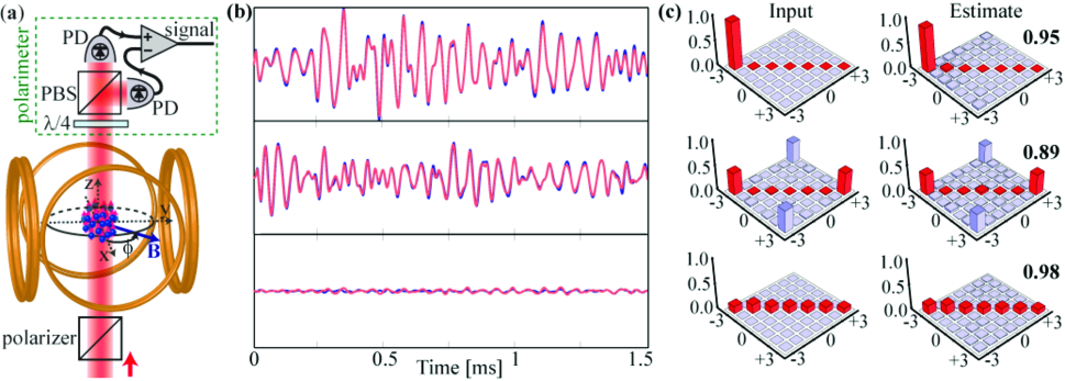
The quantum system used in our laboratory implementation is the total spin-angular momentum (electron plus nuclear) of an atom in the electronic ground state, here the hyperfine manifold of 133Cs. A detailed theoretical description of our estimation procedure and how to model this system can be found in Silberfarb et al. (2005). Our Cs ensemble is prepared by laser cooling and optical pumping, and consists of a few million atoms in a cloud with radius . The spins are coupled to the polarization of an off-resonance probe beam that serves as a meter for the measurement and can be read out in an arbitrary basis with a shot-noise limited polarimeter Smith et al. (2003), as illustrated in fig. 1a.

The spin-probe coupling depends on the atomic tensor polarizability, and can be expressed in terms of the single-atom spin F and the probe Stokes vector S,
| (1) |
where the coupling constants depend on the probe frequency, the cloud optical density, and the atomic transition Silberfarb et al. . Terms containing , , and lead to rotation of the Stokes vector around the 1, 2 and 3-axis of the Poincaré sphere, by angles proportional to the ensemble-averaged values of the respective spin observables. We use a probe initially polarized along the -axis, corresponding to an input Stokes vector , and measure the induced ellipticity, or component of the output. For the moderate optical density clouds used here all angles of rotation are small, the polarization measurement is sensitive only to rotations around the 2-axis, and the measured observable is . Coupling the entire spin ensemble to a common probe can, in principle, produce correlations between individual spins JM Geremia et al. (2004), but this effect is negligible for our optical densities.
To extract information we evolve the spins to obtain a time varying observable . Coarse-graining over time yields a discrete set and a measurement record , where Tr. Here is the quantum state to be estimated, and is a Gaussian white noise process. Full system controllability is required to make informationally complete, and can be achieved with a Hamiltonian of the form produced by a time-dependent magnetic field and the probe-induced tensor light shift (eq. 1) Smith et al. (2004). Note that for alkali atoms with an electronic ground state, the tensor light shift is proportional to the photon scattering rate and therefore comes at the cost of decoherence. By probing Cs atoms on the D1 line we achieve , enough to allow significant coherent evolution before optical pumping affects the spin state. We model our system dynamics with a master equation that fully accounts for optical pumping and experimental imperfections. The latter include bandwidth limits for our magnetic coil drivers and detection system, a 6% spatial inhomogeneity in the magnitude of the light shift which can be independently estimated, and a drift in our magnetic coil calibrations which must be included as free parameters in the estimation procedure.
We have evaluated the performance of our state estimation procedure by applying it to a range of test states. Nearly pure test states with were produced by optical pumping, and verified by Stern-Gerlach measurements of the magnetic populations. Geometric rotations of these states were obtained by Larmor precession, and more general test states were produced by evolving the system with a magnetic field and the tensor light shift. A strongly mixed state was obtained by omitting the optical pumping step and working directly with the laser cooled sample. Figure 1b compares the measurement record observed in a single ensemble interrogation to the one predicted by our model, for three representative inputs corresponding to a spin-polarized state , a coherent superposition , and a nearly maximally mixed state . Two key features are immediately apparent: the measurement records differ substantially for different input states, and the observed and calculated measurement records agree very closely. Both conditions are clearly necessary for the procedure to generate unique and accurate state estimates.
Based on our model we can determine the probability distribution for the measurement record, , conditioned on the initial quantum state and any unknown experimental parameters . We use this to obtain a maximum likelihood estimate for the state, corresponding to the peak of the posterior distribution, , where is the prior information and is a normalization constant. Here we include as prior information only that must be a physical state, i. e. a positive Hermitian operator with unit trace. The conditional distribution is a multi-parameter Gaussian centered on , the ordinary least-squares fit to the measurement record. Its covariance matrix determines the uncertainty in each of the real-valued parameters required to specify , and consequently how well an arbitrary state can be estimated. In setting up the procedure, the control magnetic field was optimized to minimize these widths and reduce their sensitivity to errors. In practice the state estimate is obtained from the measurement record in a two-step process. First we determine the least-squares fit , which is frequently non-positive due to mismatch between the modeled and actual dynamics, and then we find the positive density matrix that lies closest to . This is our maximum likelihood estimate . Figure 1c compares density matrices for the input and maximum likelihood estimates for each of our three representative test states. Visual inspection clearly shows the excellent agreement achieved by our procedure. A more quantitative performance measure can be obtained by calculating the fidelity Uhlmann (1976) which for these three states fall in the range 0.89 – 0.98. Averaging over our entire sample of test states we achieve a mean fidelity for estimates based on a single measurement record, and a slightly improved for estimates based on the average of 128 measurement records.
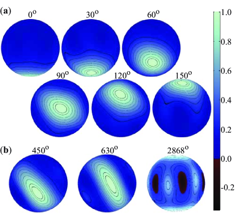
An alternative visualization of spin states can be given in terms of Wigner function representations Agarwal (1981). Figure 2a shows the estimated states for six discrete time steps during Larmor precession of an initial state .

As expected for these so-called spin-coherent states, the Wigner functions resemble Gaussian “wavepackets” moving on a sphere. A slight but visible sheering of the quasi-probability distribution occurs due to the term in the probe-induced light shift, which is expected since this is a well known mechanism for spin squeezing Kitagawa and Ueda (1993). Figure 2b shows estimated states at later times when the effects of squeezing are more pronounced. As the squeezing ellipse wraps around the sphere it eventually evolves into the coherent superposition Sanders (1989), the state used as input in fig. 1b&c. This series of snapshots demonstrates that our technique can be used to observe and visualize quite complex dynamical evolution.
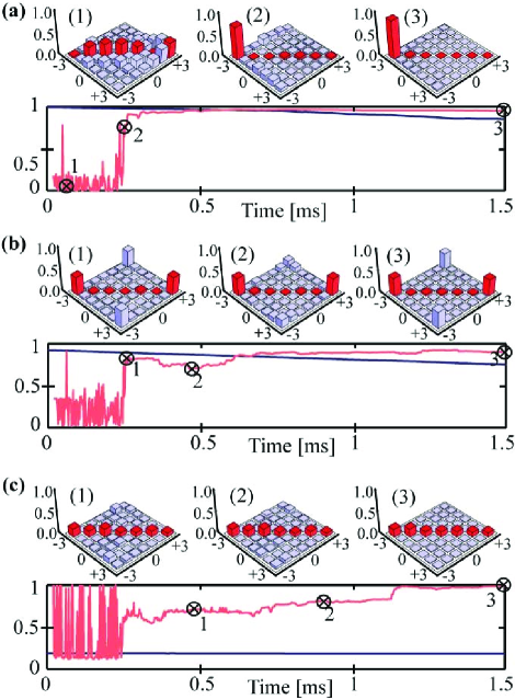
With known input states we can observe how the state estimate converges as the measurement record builds up. Figure 3 shows examples of the evolving fidelity and state estimate for pure and mixed inputs.

In all cases, the estimation starts with an unbiased guess, corresponding to a maximally mixed state. At short times, the dynamics has explored only a small part of the set , and the measurement record provides good information only about a few of the parameters that go into specifying the state. As a result the estimate fluctuates randomly with each time step, subject to noise and model/experiment discrepancies. With increasing time, the dynamics explores a larger set of observables, and the probability distributions are narrowed for every parameter. At approximately the constraints become strong enough that only a limited family of similar density matrices are consistent with the measurement record, at which point the estimate stabilizes and the fidelity improves. Figures 3a&b show the behaviors for inputs and , where the transition at brings the fidelity close to its final value. The details of the jump depend on the semidefinite program solver used to enforce positivity, but it is always dramatic for pure states where the positivity requirement excludes most nearby points in parameter space. Fig. 3c shows the behavior for an input , where most nearby points in parameter space fulfill the positivity requirement. As a result the initial jump is less dramatic and the fidelity increases more gradually to its maximum value at the end of the measurement period.
In the Heisenberg picture the state is time independent, and the estimate evolves only because more information becomes available in the measurement record. Once the measurement is complete the estimate also becomes time independent. Because the dynamics are known we can then transform to the Schrödinger picture, where the estimate becomes valid for any time, . During the measurement period there is, of course, a gradual and irreversible — but entirely predictable — loss of information from the randomizing effects of optical pumping and drive field errors. As a result an initially pure state will become mixed, and the damage can be quantified by keeping track of the largest eigenvalue of . Figure 3 shows a small decline for the input , a slightly larger decline for the more fragile superposition , and essentially no damage to the mixed state which is already randomized. Irrespective of the input state, optical pumping transfers of the ensemble into the manifold during the interrogation, but these atoms are invisible to the probe and do not contribute to the estimate or its purity.
With this work we have shown that fast, accurate and non-destructive quantum state estimation can be achieved with continuous weak measurement and dynamical control. In our current implementation the estimation fidelity is limited by imperfect control of the slowly varying magnetic field and tensor light shift used to drive the atomic spins. Our experience suggests that it may be possible to achieve far more precise control of the atomic ground state by driving the ensemble with radio-frequency and microwave radiation in the presence of a static bias magnetic field. This would eliminate optical pumping as a source of decoherence and loss, further reduce the modest loss of state purity, and make the evolution almost completely reversible. It could also allow robust state estimation without invoking extraneous parameters and the positivity requirement for , and this could shorten our data processing time from currently hour to perhaps a few seconds on a desktop computer. At that point, further improvements in the algorithm and computing hardware — for example the use of programmable logic devices Stockton et al. (2002) — could plausibly allow quantum state estimation and state-based feedback control in real time.
Acknowledgements.
This work was supported by the NSF (PHY-0355073 and PHY-0355040), ONR (N00014-05-1-0420) and NSA/DTO.References
- Nielsen and Chuang (2000) M. A. Nielsen and I. L. Chuang, Quantum Computation and Quantum Information (Cambridge University Press, Cambridge, 2000).
- Smithey et al. (1993) D. T. Smithey et al., Phys. Rev. Lett. 70, 1244 (1993); A. G. White et al., Phys. Rev. Lett. 83, 3103 (1999).
- Leibfried et al. (1996) D. Leibfried et al., Phys. Rev. Lett. 77, 4281 (1996); C. Kurtsiefer, T. Pfau, and J. Mlynek, Nature 386, 150 (1997); J. F. Kanem et al., J. Opt. B: Quant. Semiclass. Opt. 7, S705 (2005); G. Klose, G. Smith, and P. S. Jessen, Phys. Rev. Lett. 86, 4721 (2001).
- Dunn et al. (1995) T. J. Dunn, I. A. Walmsley, and S. Mukamel, Phys. Rev. Lett. 74, 884 (1995); E. Skovsen et al., Phys. Rev. Lett. 91, 090406 (2003); I. L. Chuang, N. Gershenfeld, and M. Kubinec, Phys. Rev. Lett. 80, 3408 (1998).
- Silberfarb et al. (2005) A. Silberfarb, P. S. Jessen, and I. H. Deutsch, Phys. Rev. Lett 95, 030402 (2005).
- Doherty et al. (2000) A. C. Doherty et al., Phys. Rev. A 62, 012105 (2000); S. Lloyd and J. E. Slotine, Phys. Rev. A 62, 012307 (2000).
- Smith et al. (2003) G. A. Smith, S. Chaudhury, and P. S. Jessen, J. Opt. B: Quant. Semiclass. Opt. 5, 323 (2003).
- (8) A. Silberfarb, P. S. Jessen, and I. H. Deutsch, to be published. See also JM Geremia, J. K. Stockton, and H. Mabuchi, Phys. Rev. A 73, 042112 (2006).
- JM Geremia et al. (2004) JM Geremia, J. K. Stockton, and H. Mabuchi, Science 304, 270 (2004).
- Smith et al. (2004) G. A. Smith et al., Phys. Rev. Lett. 93, 163602 (2004).
- Uhlmann (1976) A. Uhlmann, Rep. Math. Phys. 9, 273 (1976).
- Agarwal (1981) G. S. Agarwal, Phys. Rev. A 24, 2889 (1981).
- Kitagawa and Ueda (1993) M. Kitagawa and M. Ueda, Phys. Rev. A 47, 5138 (1993).
- Sanders (1989) B. Sanders, Phys. Rev. A 40, 2417 (1989).
- Stockton et al. (2002) J. Stockton, M. Armen, and H. Mabuchi, J. Opt. Soc. Am. B 19, 3019 (2002).