Semi-spectral Chebyshev method in Quantum Mechanics

Abstract

Traditionally, finite differences and finite element methods have been by many regarded as the basic tools for obtaining numerical solutions in a variety of quantum mechanical problems emerging in atomic, nuclear and particle physics, astrophysics, quantum chemistry, etc. In recent years, however, an alternative technique based on the semi-spectral methods has focused considerable attention. The purpose of this work is first to provide the necessary tools and subsequently examine the efficiency of this method in quantum mechanical applications. Restricting our interest to time independent two-body problems, we obtained the continuous and discrete spectrum solutions of the underlying Schrödinger or Lippmann-Schwinger equations in both, the coordinate and momentum space. In all of the numerically studied examples we had no difficulty in achieving the machine accuracy and the semi-spectral method showed exponential convergence combined with excellent numerical stability.

I Introduction

The exact solutions of the Schrödinger equation are known to exist only in a few rather idealized examples. Since in all remaining cases one has to be content with the numerically generated solutions, the importance of numerical methods in quantum mechanics can hardly be overestimated. Broadly speaking, one may distinguish two schools of thought fornberg boyd : (i) the local approach comprising the finite differences and finite element methods, and, (ii) the global approach encompassing a variety of spectral methods. The local methods usually require much larger grids than other methods as the convergence of these schemes is generally algebraic. By contrast, the global methods have been shown to provide exponential convergence delivering smooth solutions which in most cases are preferable.

The local methods approximate the unknown function by a sequence of overlapping low order polynomials which are used to interpolate the function at a small sub-set of the grid points. The derivative of the unknown function is then approximated by the derivative of the interpolating polynomial so that the former takes the form of a weighted sum of the function values at the interpolation points. The method is designed to be exact for polynomials of low order and the form of the difference quotient is chosen such that certain order of the truncation error is maintained (in the lowest order $\textstyle{\rm d}u(x)/\textstyle{\rm d}x\approx[u(x+h)-u(x-h)]/(2h)+O(h^{2})$ where $h$ is a small grid spacing). In the simplest version this procedure converts a differential equation into a three-term recurrence, as may be exemplified by the popular Numerov algorithm taopang , easy to program and implement but relatively low in accuracy.

The strategy of the global or spectral methods is very different. Here, the unknown function is sought in the form of a generalized Fourier expansion, truncated for practical reasons, using global basis functions which usually are polynomials or trigonometric polynomials of a high degree. This approach may be viewed as the limit of the finite difference method whose order of accuracy has been pushed to infinity.

The semi-spectral Chebyshev method – a prominent representative of the global approach – provides effective means to solve a generic equation of the form $L\,u(x)=f(x)$ where the independent variable $x$ belongs to some interval $[a,b]$, $L$ is a differential or integral operator, $f(x)$ is a given function and $u(x)$ is the unknown function satisfying some, as yet unspecified boundary conditions. For the sake of simplicity of the exposition we consider just a single independent variable $x$. The underlying idea is exceedingly simple: to obtain the solution, first the problem is discretized by introducing a grid consisting of $N$ points $t_{i}\in[a,b],\,i=1,2,\dots N$, then the underlying equation is solved exactly at all of the grid points, and, finally with the solutions $u(t_{i})$ in hand, an interpolating procedure is invoked to get $u(x)$ at an arbitrarily chosen $x$ value. Obviously, the key issue here would be the choice of the grid and the interpolation method but it turns out that the scheme based on Chebyshev polynomials provides the best offer on both accounts. It would be instructive to compare this approach with other methods and put it in a historical perspective but this is not so simple because the abundant mathematical literature is lacking a generally accepted standardization boyd and quite often different methods bear the same tag, or else, the same thing appears under different names. Accordingly, the semi-spectral method might be called orthogonal collocation, Petrov-Galerkin, or even Rayleigh-Ritz method. The common point of departure in all of the methods is the effort to minimize the error distribution given by the reminder or the residue function $R(x)\equiv L\,u(x)-f(x)$ and there is a number of possible strategies to achieve this goal. It is convenient to seek the solution as a superposition of some trial functions $\phi_{i}(x)$

$$u(x)=\sum_{i=1}^{N}c_{i}\,\phi_{i}(x),$$ (1)

where $c_{i}$ are hitherto unknown generalized Fourier expansion coefficients. The trial functions are expected to be easy to get by apart from the usual indispensable requirements of completeness and orthogonality. Local methods like finite difference or finite element methods use for this purpose low order partially overlapping polynomials defined on a grid whereas the global methods employ trigonometric functions (Fourier methods) or high order polynomials spanning over the whole domain. The global methods are also known as the spectral methods. In order to minimize the residue function another set of the so called test functions $\chi_{i}(x)$ is needed together with a definition of a scalar product of two functions $f(x)$ and $g(x)$ which is taken to be given as

$$(f,g)=\int_{a}^{b}f(x)\,g(x)\,\rho(x)\,\textstyle{\rm d}x,$$ (2)

where $\rho$ is a weighting function and the interval $[a,b]$ specifies the domain. When $u$ were the exact solution the residue function would identically vanish but with an approximate solution we can only try making the error distribution as small as possible by minimizing the residue function. This can be effected by stipulating the conditions $(R,\chi_{i})=0,\;i=1,2,\dots N$. Indeed, since the test functions form a complete set, the vector $R$ orthogonal to all members of such a set must be a null vector. The above orthogonality conditions lead to a linear set of algebraic equations

$$\sum_{i=1}^{N}(\chi_{j},L\phi_{i})c_{i}=(\chi_{j},f),\quad j=1,2,\dots N$$ (3)

for the expansion coefficients $c_{i}$ which can be solved by standard methods. It will be convenient to distinguish three possible implementations of the above scheme.

1. Semi-spectral method. A grid $t_{i}$ is introduced and the test functions are adopted in the form $\chi_{i}(x)=\delta(x-t_{i})$.

2. Galerkin, or spectral method. The test functions and the trial functions are identical $\chi_{i}(x)=\phi_{i}(x)$ for all $i$.

3. Petrov-Galerkin method. The test functions and the trial functions are different.

It has to be noted that the grid is indispensable only in the semi-spectral method whereas the remaining two methods can do without it. In the following we shall concentrate on the semi-spectral and the Galerkin method.

As far as the basis functions are concerned, it is a common practice taking for $\phi_{j}(x)$ any of the sets of the orthogonal polynomials collected in abramowitz . Indeed, since all of them result as eigenfunctions of a certain Sturm-Liouville problem their completeness and orthogonality are guaranteed. There are also additional advantages following from taking polynomials as the expansion basis: firstly, this immediately sets an important correspondence linking the generalized Fourier expansion with an interpolating scheme, and, secondly, it simplifies all the necessary integrations by using the highly accurate Gauss integration scheme. We shall take on both of these issues, assuming that from now on $\phi_{j}(x)$ stands for a polynomial of the order $(j-1)$. For an approximation of the order $N$ and assigned polynomial type the grid points $t_{j},\;j=1,2,\dots N$ will be identical with the Gauss abscissas which are given as the zeros of the polynomial $\phi_{N+1}(x)$.

Integration. The Gauss integration formula, takes the form

$$\int_{a}^{b}u(x)\,\rho(x)\,\textstyle{\rm d}x=\displaystyle\sum_{j=1}^{N}w_{j}\,u(t_{j})$$ (4)

and is known to be exact if $u(x)$ is a polynomial whose order is not greater than $(2\,N+1)$. The weights $w_{j},\,j=1,2,\dots N$ are obtained by solving the linear system

$$\sum_{j=1}^{N}t_{j}^{n}\,w_{j}=\int_{a}^{b}x^{n}\,\rho(x)\,\textstyle{\rm d}x;\quad n=0,1,\dots(N-1).$$ (5)

Interpolation. The truncated Fourier expansion can be converted into an interpolative formula with the aid of the cardinal function $G_{j}(x)$ with the property $G_{j}(t_{i})=\delta_{ij}$. This function can be obtained by construction

$$G_{j}(x)=\phi_{N+1}(x)/[\phi^{\prime}_{N+1}(t_{j})(x-t_{j})]$$ (6)

where prime denotes the derivative and the interpolative formula reads

$$u(x)=\sum_{j=1}^{N}\,u(t_{j})\,G_{j}(x).$$ (7)

The cardinal function is a polynomial of order $(N-1)$ and may be written as a superposition of the basis functions

$$G_{j}(x)=\sum_{i=1}^{N}M_{ji}^{-1}\,\phi_{i}(x)$$ (8)

where the coefficient matrix $\bm{M}^{-1}$ can be determined by taking advantage of the orthogonality of the basis. Using the Gauss integration formula, we obtain

$$M^{-1}_{ij}=\phi_{i}(t_{j})\,w_{j}/(\phi_{i},\phi_{i})$$ (9)

This matrix can be immediately inverted by applying Gauss integration formula for expressing the orthogonality condition for the basis

$$\int_{a}^{b}\phi_{i}x)\,\phi_{k}(x)\,\rho(x)\,\textstyle{\rm d}x=\delta_{ik}(\phi_{i},\phi_{i})=\displaystyle\sum_{j=1}^{N}\phi_{i}(t_{j})\,w_{j}\,\phi_{k}(t_{j})$$ (10)

and this result is exact. Since the orthogonality condition has here the form $\bm{M}^{-1}\cdot\bm{M}=\bm{1}$, it remains to read off the the matrix $\bm{M}$

$$M_{ij}=\phi_{j}(t_{i}).$$ (11)

The function $u(x)$ is determined by supplying the coefficients $c_{j}$ occurring in the spectral expansion formula but the latter is completely equivalent to the interpolative formula that instead of the $c_{j}$ employs the grid values $u(t_{j})$. There is a linear relation between these two arrays provided by the $\bm{M}$ matrix which can be written in a concise form

$$[u]=\bm{M}\cdot[c].$$ (12)

The array of the coefficients $[c]$ is obtained by solving the linear system (3). In the semi-spectral method, this gives

$$\sum_{j=1}^{N}\{L\phi_{j}(x)\}_{x=t_{i}}\,c_{j}=f(t_{i}),\quad i=1,2,\dots N$$ (13)

whereas the Galerkin scheme yields

$$\sum_{j=1}^{N}(\phi_{k},L\phi_{j})\,c_{j}=(\phi_{k},f),\quad k=1,2,\dots N$$ (14)

However, if the integration in (14) is effected by the Gauss method, the resulting equations in both, semi-spectral and Galerkin schemes turn out to be identical and the two methods are completely equivalent. Indeed, multiplying both sides of (13) by $\phi_{k}(t_{i})\,w_{i}$ and carrying out a summation over $i$, we immediately obtain (14). In many applications the interpolative form (7) might be more convenient, in which case $u(t_{j})$ play the role of the unknowns. The latter are determined by solving the linear system

$$\sum_{j=1}^{N}\{L\,G_{j}(x)\}_{x=t_{i}}\,u(t_{j})=f(t_{i}),\quad i=1,2,\dots N$$ (15)

The resulting $u(t_{j})$ are subsequently used in (7) to obtain the ultimate solution of the problem, as advertised at the beginning of this section.

In this paper we are going to use the Chebyshev polynomials as the basis functions. There are strong arguments corroborating this choice. Firstly, the Chebyshev polynomials optimize the interpolative procedure, as will be discussed shortly. Secondly, the values of the grid points $t_{j}$ for all $N$ are given by an elementary analytic expression whereas for other polynomials they would have to be computed numerically for every $N$. Thirdly, the Fourier coefficients of the function and the appropriate coefficients specifying the derivative are connected by a simple linear transformation. Fourthly, the same is true for the antiderivatives. Simplifying matters, one may say that by differentiating or integrating a set of Chebyshev polynomials we always obtain a set of Chebyshev polynomials and therefore these operations can be reduced to simple matrix manipulations. In the next Section we have presented all the necessary tools for solving some typical differential and integral equations occurring in quantum mechanics. Subsequently, we consider the application of the semi-spectral Chebyshev method. Due to space limitations some selection was inevitable and we decided to confine our interest to the time independent non-relativistic two-body problems. We concentrate our attention on the situation when the forces take the form of a short ranged potential considering in sequence the continuous and the discrete spectrum. The solutions are obtained both in configuration and in momentum space using the appropriate Schrödinger, or the Lippmann-Schwinger (from now on referred to as L-S) equation, with and without the Coulomb interaction. These kind of problems are often encountered in nuclear and particle physics and we offer a variety of complete solutions.

In the last part we present some numerically solved examples. The short-range interaction is modelled by three different spherically symmetric potentials. The first of them, the exponential potential can be viewed as the simplest prototype of the forces rapidly falling off with the distance morsefeshbach . More complicated shapes can be obtained by taking suitable superpositions of exponential potentials with different ranges. Our second choice, the Morse potential morse , is a particular combination of two exponential potentials of different ranges where one of them is repulsive while the other is attractive. This potential has been very popular rawitscher02 as a model for vibrational states of diatomic molecules but it has been also used in nuclear physics to simulate a repulsive core nucleon-nucleon interaction darewychgreen . As the other extreme one may take an infinite superposition of exponential potentials forming a geometric series. The explicit summation of this series leads to our third choice, the familiar Hulthén potential hulthen which close to the origin develops a $1/r$ singularity, like the Coulomb potential, and yet exhibits an exponential fall-off at large distances. The meaning of the Hulthén potential goes far beyond academic interest as it has been widely used in nuclear and particle phenomenology durand vandijk , atomic physics solid state lamvarshni , quantum chemistry olsonmicha etc. Here, for us the important fact is that for $L=0$ all the three potentials mentioned above admit analytic solutions and the situation has been summarized in the Appendix morsefeshbach fluge . In most instances the semi-spectral method turns out to be so accurate that the standard procedure, where the convergence is examined by comparison with the results obtained by ”other methods”, almost certainly would be meaningless. Therefore, for calculating the relative errors we always utilized the exact results.

II Chebyshev interpolation

II.1 Chebyshev cardinal function

Let us consider an independent variable $t$ defined in the $[-1,1]$ interval (our conventions and notation in this section are consistent with recipes ) The Chebyshev polynomial $T_{N}(t)$ of the first kind and of degree $N$ is defined mason rivlin by the formula

$$T_{N}(t)=\cos(N\arccos(t)).$$ (16)

It is evident that $T_{N}(t)$ has $N$ zeros in the $[-1,1]$ interval and they are located at the points

$$t_{k}=\cos[\pi(k-\textstyle\frac{1}{2})/N];\quad k=1,2,\dots,N$$ (17)

The Chebyshev polynomials can be also generated from the recurrence relation

$$T_{n}(t)=2t\,T_{n-1}(t)-T_{n-2}(t)$$

with $T_{0}(t)=1$ and $T_{1}(t)=t$. The Chebyshev polynomials of the second kind, denoted as $U_{n}(t)$, are obtained from the same recurrence relation but with different starting values: $U_{-1}(t)=0$ and $U_{0}(t)=1$.

Usually, two choices of grids are considered: (i) the classical Chebyshev mesh-points given in (17), or, (ii) the zeros of the derivatives of $T_{N}(t)$ which is the same as the zeros of $U_{N-1}(t)$. The choice (ii) is called Lobatto mesh, for it was shown by Lobatto that the zeros of the derivative $T^{\prime}_{N}(t)$ supplemented by the end-points $\pm 1$ have all the advantageous features of the Chebyshev mesh. Furthermore, if a function is approximated by Chebyshev polynomials supplying the boundary values of the function immediately pins down two coefficients. The other attractive feature shows up when the Lobatto mesh is used in quadratures and when $N$ and subsequently $2N$ points are taken to obtain useful and computable error estimate. In the bigger mesh half of the points coincide with those of the smaller mesh and therefore the function values calculated at the smaller mesh can be later reused reducing thereby the total number of function evaluation. The Lobatto mesh, however, is not always preferable and especially for functions which exhibit end-point singularities more convenient might be the classical Chebyshev mesh. Apart from personal prejudices, there is little difference between these two schemes in terms of accuracy, or convergence boyd .

The Chebyshev polynomials are orthogonal in the interval $[-1,1]$ over a weighting factor $1/\sqrt{1-t^{2}}$ and from the continuous orthogonality relation a discrete orthogonality relation can be derived. In this work we shall use the classical Chebyshev mesh (17) and the appropriate orthogonality relations, take the form

$$\dfrac{\pi}{N}\sum_{k=1}^{N}T_{i}(t_{k})\,T_{j}(t_{k})=\delta_{ij}\;\dfrac{\pi}{2}(1+\delta_{0i})$$ (18)

where $i<N$ and $j<N$.

A continuous and bounded function $f(t)$ can be approximated in $[-1,1]$ interval by the expression

$$f(t)=\sum_{j=1}^{N}{\rm{}^{\prime}\mbox{}}\ c_{j}\,T_{j-1}(t)$$ (19)

where the primed sigma denotes hereafter a summation in which the first term should be halved. The spectral coefficients $c_{j}$ can be obtained by multiplying (19) by $T_{i-1}(t)$ and then setting $t$ equal to $t_{k}$ and, finally, performing a summation over $k$. Making use of (18), we get

$$c_{j}=\dfrac{2}{N}\sum_{k=1}^{N}\,M_{jk}\,f(t_{k}),$$ (20)

with $M_{jk}=T_{j-1}(t_{k})$ where

$$T_{j-1}(t_{k})=\cos[\pi(k-\textstyle\frac{1}{2})(j-1)/N].$$ (21)

We may regard (19) as a generalized truncated Fourier expansion. Recalling that $T_{N}(t)$ vanishes at all $t=t_{j}$, (19) can be rewritten as

$$f(t)=\sum_{j=1}^{N}\dfrac{T_{N}(t)}{T_{N}^{\prime}(t_{j})(t-t_{j})}\;f(t_{j}),$$ (22)

where prime stands for the derivative. This is nothing else but an interpolating formula, which may be cast to the familiar Lagrange form

$$f(t)=\sum_{j=1}^{N}\;G_{j}(t)\;f(t_{j}),$$ (23)

where we have introduced the Chebyshev cardinal functions $G_{j}(t)$, with the property $G_{j}(t_{i})=\delta_{ij}$. Indeed, inserting (20) into (19), we obtain

$$G_{j}(t)=\dfrac{2}{N}\sum_{i=1}^{N}{\rm{}^{\prime}\mbox{}}\ T_{i-1}(t_{j})\,T_{i-1}(t).$$ (24)

It is evident that there are two options for reconstructing the function $f(t)$: either from the expansion (19) knowing the coefficients $c_{i}$, or by supplying the values of $f(t_{j})$ and using (23). These options are completely equivalent and knowing the mesh-point values $f(t_{j})$ of the function, the corresponding Fourier coefficients can be obtained from (20).

Similar procedure may be applied for a function of two, or more, variables. Thus, a simple extension of (23) to the case when the function depends upon two variables $x$ and $y$, is

$$f(x,y)=\sum_{i,j=1}^{N}\;G_{i}(x)\;f(t_{i},t_{j})\;G_{j}(y).$$ (25)

Owing to their rapid, often exponential, convergence rate when the number of mesh-points $N$ increases, the Chebyshev interpolation methods have proved to be extremely efficient in solving various problems of mathematical physics. This success has a very solid background resting on two celebrated theorems which we quote here without proof boyd .

Theorem 1 (Cauchy interpolation error theorem).

Let $f(t)$ be a function sufficiently smooth so that it has at least $N+1$ continuous derivatives on the interval $[-1,1]$ and let $P_{N}(t)$ be its Lagrangian interpolant of degree $N$ for $t\in[-1,1]$. Then, for any grid ${t_{i}}\in[-1,1]$ and any $t\in[-1,1]$ the upper bound of the interpolation error is given by

$$f(t)-P_{N}(t)\leq\dfrac{1}{(N+1)!}\;f^{(N+1)}(\xi)\;\prod_{i=1}^{N}(t-t_{i})$$ (26)

for some $\xi(t)\in[a,b]$.

It is worth noting that the product term in (26) is itself a monic polynomial (leading term coefficient equal unity). The above Cauchy theorem indicates that without specifying the function $f(t)$, the only way to minimize the interpolation error is to minimize the product term in (26) and this in turn can be achieved by a judicious choice of the interpolation points. The answer how to accomplish that brings the following Chebyshev theorem boyd .

Theorem 2 (Chebyshev minimal amplitude theorem).

Out of all monic polynomials of degree $N$, the unique polynomial which has the smallest maximum on $[-1,1]$ is the Chebyshev polynomial $T_{N}(t)$ divided by $2^{N-1}$, i.e. all monic polynomials $Q_{N}(t)$ of degree $N$ satisfy the inequality

$$\max|Q_{N}(t)|\geq\max|T_{N}(t)/2^{N-1}|=1/2^{N-1}$$ (27)

for all $t\in[-1,1]$.

II.2 Anti-derivative

The optimized interpolation is highly satisfactory but there is much more to come. As we shall see in a moment, by using the spectral representation simple operations like differentiation or integration can be reduced to matrix multiplication. We start with integration, introducing the anti-derivative of $f(t)$, defined as

$$F^{-}(t)=\int_{-1}^{t}\,f(x)\,\textstyle{\rm d}x.$$ (28)

The anti-derivative might be sought in the form of an appropriate Chebyshev expansion

$$F^{-}(t)=\sum_{j=1}^{N}{\rm{}^{\prime}\mbox{}}\ C_{j}\,T_{j-1}(t).$$ (29)

in which case our objective would be to calculate the coefficients $C_{j}$ occurring in (29). If the function in the integrand of (28) is represented by its Chebyshev expansion (19), the integration in (28) can be done analytically (Curtis-Clenshaw integration clenshaw ). This solves the problem because the coefficients $C_{j}$ in (29) must be expressible in terms of $c_{j}$ but these relations are not particularly simple. El-gendi observed elgendi that much simpler relations would be obtained if instead of the spectral coefficients the function values at the mesh-points were used elgendi mihaila . In the latter case the array of the mesh values of the anti-derivative $F^{-}(t_{i})$ would be connected with the array of the integrand mesh values $f(t_{j})$ by a simple linear transformation which bears a universal character being independent upon the shape of $f(t)$. Indeed, by inserting (23) in (28), we end up with a remarkably simple quadrature rule

$$F^{-}(t_{i})=\sum_{j=1}^{N}\ W^{-}_{ij}\,f(t_{j})$$ (30)

where $W^{-}_{ij}$ may be viewed as a generalized weighting factor. For a fixed $N$, this is a constant matrix, viz.

$$W^{-}_{ij}=\int_{-1}^{t_{i}}\,G_{j}(t)\,\textstyle{\rm d}t$$ (31)

which will be obtained in an analytic form. Inserting (24) in (31), we get

$$W^{-}_{ij}=\dfrac{2}{N}\sum_{k=1}^{N}{\rm{}^{\prime}\mbox{}}\ \int_{-1}^{t_{i}}\,T_{k-1}(t)\,\textstyle{\rm d}t\;T_{k-1}(t_{j})$$ (32)

and, as seen from (32), the matrix $\bm{W}^{-}$ may be written as a product $\bm{W}^{-}=\bm{S}^{-}\cdot\bm{d}^{-1}\cdot\bm{M}$, where $\bm{M}$ is given in (21), $\bm{d}=\text{diag}(N,\,\textstyle\frac{1}{2}N,\,\textstyle\frac{1}{2}N,\,\dots,\,\textstyle\frac{1}{2}N)$, and $\bm{S}^{-}$, is

$$S^{-}_{ij}=\int_{-1}^{t_{i}}\,T_{j-1}(t)\,\textstyle{\rm d}t.$$ (33)

The integral in (33) can be obtained from an analytic expression

$$\int_{-1}^{t_{i}}\,T_{j-1}(t)\,\textstyle{\rm d}t=\begin{cases}T_{1}(t_{i})+1;\quad&\text{for $j=1$}\\ [T_{2}(t_{i})-1]/4;\quad&\text{for $j=2$}\\ T_{j}(t_{i})/(2j)-T_{j-2}(t_{i})/2(j-2)+(-1)^{j}/j(j-2);\quad&\text{for $j>2$}\end{cases}$$ (34)

where the right hand sides of (34) are readily computed with the aid of (21). It is worth noting that the discrete orthogonality relation (18) can be written in matrix form as $\bm{M}\cdot\tilde{\bm{M}}=\bm{d}$ with tilde denoting the transposed matrix. Since the matrix $\bm{M}$ has orthogonal columns, we have $\bm{M}^{-1}=\tilde{\bm{M}}\cdot\bm{d}^{-1}$. When the array $F^{-}(t_{i})$ has been determined, the expansion coefficients of the anti-derivative may computed from

$$C_{i}=\dfrac{2}{N}\sum_{j=1}^{N}\,M_{ij}\,F^{-}(t_{j})$$ (35)

and the anti-derivative $F^{-}(t)$ could be reconstructed at any point either from (29), or from (23) after making the substitution $f\to F^{-}$.

Alternatively, we could have defined the anti-derivative as

$$F^{+}(t)=-\int_{t}^{1}\,f(x)\,\textstyle{\rm d}x$$ (36)

in which case the appropriate integration rule, takes the form

$$F^{+}(t_{i})=-\sum_{j=1}^{N}\ W^{+}_{ij}\,f(t_{j})$$ (37)

where $\bm{W}^{+}=\bm{S}^{+}\cdot\bm{d}^{-1}\cdot\bm{M}$ and for $\bm{S}^{+}$, we obtain

$$\int_{t_{i}}^{1}\,T_{j-1}(t)\,\textstyle{\rm d}t=\begin{cases}-T_{1}(t_{i})+1;\quad&\text{for $j=1$}\\ -[T_{2}(t_{i})-1]/4;\quad&\text{for $j=2$}\\ -T_{j}(t_{i})/(2j)+T_{j-2}(t_{i})/2(j-2)-1/j(j-2);\quad&\text{for $j>2$}\end{cases}$$ (38)

In the following we shall need both forms of the anti-derivatives.

II.3 Integration

A definite integral in the $[-1,1]$ limits might be calculated in a similar way as the anti-derivative but we wish to consider the numerical evaluation of a slightly more general integral

$$I[f]=\int_{-1}^{1}\,k(t)\,f(t)\,\textstyle{\rm d}t$$ (39)

where $k(t)$ is a real absolutely integrable function, which need not be continuous or of one sign, while $f(t)$ is any continuous function. The integration will be performed by using the product integration form

$$I_{N}[f]=\sum_{i=1}^{N}\,w_{i}\,f(t_{i})$$ (40)

where the weights $w_{i}$ are determined by requiring the above rule to be exact when $f(t)$ is any polynomial of degree $\leq N$. This can be regarded as a variation of the Clenshaw-Curtis integration and indeed reduces to that method when the mesh-points are taken to be the Lobatto points an $k(t)$ is set to unity. It has been shown sloan that the integration rule (40) for $N\to\infty$ converges to the exact result for all continuous functions $f(t)$, provided $k(t)$ satisfies a rather mild integrability condition, namely

$$\int_{-1}^{1}\,|k(t)|^{p}\,\textstyle{\rm d}t<\infty$$ (41)

for some $p>1$. Two choices of $k(t)$ are of particular interest. The first is when $k(t)$ is taken to be the Chebyshev weighting function $k(t)\equiv 1/\sqrt{1-t^{2}}$ and we end up with the standard Gauss-Chebyshev quadrature abramowitz

$$\int_{-1}^{1}\,f(t)\,\dfrac{\textstyle{\rm d}t}{\sqrt{1-t^{2}}}=\dfrac{\pi}{N}\displaystyle\sum_{j=1}^{N}\,f(t_{j}),$$ (42)

with $w_{j}=\pi/N$ for all $j$. The second case of practical interest is that in which $k(t)\equiv 1$ and we have

$$\int_{-1}^{1}\,f(t)\,\textstyle{\rm d}t=\displaystyle\sum_{j=1}^{N}\,w_{j}\,f(t_{j})$$ (43)

with the Chebyshev weights

$$w_{j}=\dfrac{2}{N}\sum_{k=1}^{N}{\rm{}^{\prime}\mbox{}}\ T_{k-1}(t_{j})\int_{-1}^{1}\,T_{k-1}(t)\,\textstyle{\rm d}t.$$ (44)

The integral occurring in (44) can be easily evaluated, viz.

$$\int_{-1}^{1}\,T_{k-1}(t)\,\textstyle{\rm d}t=[(-1)^{k}-1]/[k(k-2)]$$ (45)

and inserting (45) in (44), we arrive at the ultimate expression for the weights

$$w_{j}=-\dfrac{4}{N}\;\;\sideset{}{\,{}^{\prime}}{\sum}_{i=0}^{[(N-1)/2]}\;\;\dfrac{T_{2i}(t_{j})}{4i^{2}-1}.$$ (46)

It can be proved that the weights (46) are all positive and setting $f(t)\equiv 1$ in (43), we obtain the sum rule

$$\sum_{i=1}^{N}w_{i}=2.$$

II.4 Singular integrals

The Chebyshev quadrature can be extended to comprise also singular integrals. To this end we consider product integration (39) in which $k(t)$ may contain isolated singularities hasegawa . Perhaps the most important of them is the Cauchy integral, and we wish to establish the quadrature rule for the principal value integral of the form

$$\int_{-1}^{1}\dfrac{f(t)}{t-z}\,\textstyle{\rm d}t=\displaystyle\sum_{j=1}^{N}\omega_{j}(z)\,f(t_{j})$$ (47)

where the weights $\omega_{j}(z)$ depend upon the location of the singularity. It is assumed in the following that $|z|<1$ and that the function $f(t)$ is free from singularities on the $<-1,1>$ interval of the real axis. Our goal is to calculate the generalized weights $\omega_{j}(z)$ and inserting (23) in the left hand side of (47), we have

$$\omega_{j}(z)=\dfrac{2}{N}\sum_{k=1}^{N}{\rm{}^{\prime}\mbox{}}\;T_{k-1}(t_{j})\,I_{k-1}(z)$$ (48)

with $I_{k-1}(z)$ denoting the principal value integral

$$I_{k-1}(z)=\int_{-1}^{1}\dfrac{T_{k-1}(t)}{t-z}\,\textstyle{\rm d}t$$ (49)

which will be calculated in an analytic form. Indeed, a simple subtraction, yields

$$\int_{-1}^{1}\dfrac{T_{k-1}(t)}{t-z}\,\textstyle{\rm d}t=\displaystyle\int_{-1}^{1}\dfrac{T_{k-1}(t)-T_{k-1}(z)}{t-z}\,\textstyle{\rm d}t+T_{k-1}(z)\,\log{\dfrac{1-z}{1+z}}$$ (50)

and the integrand on the right hand side of (50) being now regular, can be represented as a superposition of Chebyshev polynomials

$$\dfrac{T_{k-1}(t)-T_{k-1}(z)}{t-z}=2\sum_{i=0}^{k-2}{\rm{}^{\prime}\mbox{}}\;U_{k-2-i}(z)\,T_{i}(t)$$ (51)

rendering the t-integration straightforward. With the aid of (45), we obtain the ultimate expression

$$I_{k-1}(z)=S_{k-1}(z)+T_{k-1}(z)\,\log{[(1-z)/(1+z)]};$$ (52)

with

$$S_{k-1}(z)\equiv-2\displaystyle\sum_{i=0}^{k-2}{\rm{}^{\prime}\mbox{}}\;\dfrac{(-1)^{i}+1}{i^{2}-1}\;U_{k-2-i}(z)$$ (53)

and (52)-(53) used in (48) allows to calculate explicitly the weights. The presence of the end-point logarithmic singularities is apparent in (52) and at these values the principal value integral (49) becomes undefined. It is interesting to note that the relation between the function $I_{n}(z)$ and $T_{n}(z)$ is analogous to that between the Legendre function $Q_{n}(z)$ and the Legendre polynomial $P_{n}(z)$. It will be convenient to separate the singular term writing the weights in the form

$$\omega_{j}(z)=\tilde{\omega}_{j}(z)+G_{j}(z)\,\log{[(1-z)/(1+z)]};$$ (54)

where $G_{j}(z)$ is the cardinal function and the regular part, given by

$$\tilde{\omega}_{j}(z)=\dfrac{2}{N}\sum_{k=1}^{N}{\rm{}^{\prime}\mbox{}}\;T_{k-1}(t_{j})\,S_{k-1}(z)$$ (55)

is just a polynomial in $z$. The ultimate quadrature rule for a general integral of the Cauchy type, reads

$$\int_{-1}^{1}\dfrac{f(t)\,\textstyle{\rm d}t}{t-z\mp\textstyle{\rm i}\epsilon}=\begin{cases}\displaystyle\sum_{j=1}^{N}\dfrac{w_{j}}{t_{j}-z}\,f(t_{j}),&|z|>1\\ \displaystyle\sum_{j=1}^{N}\tilde{\omega}_{j}(z)\,f(t_{j})+f(z)\left(\log{\dfrac{1-z}{1+z}}\pm\textstyle{\rm i}\pi\right).&|z|<1\end{cases}$$ (56)

Setting $f(t)\equiv 1$ in (47), a sum rule is obtained

$$\sum_{j=1}^{N}\omega_{j}(z)=\log{\dfrac{1-z}{1+z}}$$

providing a convenient check of the computed weights.

The other important case to be considered here is that of the logarithmic singularity. The appropriate automatic quadrature, takes the form

$$\int_{-1}^{1}f(t)\,\log{|t-z|}\,\textstyle{\rm d}t=\begin{cases}\displaystyle\sum_{j=1}^{N}w_{j}\,f(t_{j})\log{|t_{j}-z|},&|z|>1\\ \displaystyle\sum_{j=1}^{N}\Omega_{j}(z)\,f(t_{j}),&|z|\leq 1\end{cases}$$ (57)

and our goal is to determine the weights $\Omega_{j}(z)$. The assumptions concerning $f(t)$ and $z$ remain the same as in the Cauchy integral case (47). In particular, for the time being, we assume that $|z|\neq 1$ but eventually this restriction will be lifted. Upon inserting (23) in the left hand side of (57), the dedicated weights $\Omega_{j}(z)$ can be written in the form

$$\Omega_{j}(z)=\dfrac{2}{N}\sum_{k=1}^{N}{\rm{}^{\prime}\mbox{}}\;T_{k-1}(t_{j})\,J_{k-1}(z)$$ (58)

with $J_{k-1}(z)$ denoting the integral

$$J_{k-1}(z)=\int_{-1}^{1}T_{k-1}(t)\;\log{|t-z|}\,\textstyle{\rm d}t,$$ (59)

which can be evaluated analytically. In order to do that, we take advantage of the identity rivlin which holds for non-negative $n$

$$T_{n}(t)=\begin{cases}\dfrac{1}{2(n+1)}\,T_{n+1}^{\prime}(t)-\dfrac{1}{2(n-1)}\,T_{|n-1|}^{\prime}(t),\quad&n\neq 1\\ \frac{1}{4}\,T_{2}^{\prime}(z),&n=1.\end{cases}$$

with prime denoting the derivative. Inserting the above identity in (59), the integration by parts, gives

$$J_{k-1}(z)=\begin{cases}-\dfrac{\log{|1-z|}-(-1)^{k}\log{|1+z|}}{k(k-2)}-\dfrac{I_{k}(z)}{2k}+\dfrac{I_{|k-2|}(z)}{2(k-2)},&k\neq 2\\ \frac{1}{4}\left\{\log{\left|\dfrac{1-z}{1+z}\right|}-I_{2}(z)\right\},&k=2,\end{cases}$$ (60)

where $k=1,2,\cdots,N$. Substituting the explicit forms of $J_{k-1}(z)$ in (58) completes the derivation of the weighting functions $\Omega_{j}(z)$.

The integral containing a logarithmic singularity (57), unlike the Cauchy integral, does exist even when the singularity coincides with either of the integration end points. Therefore, all $J_{k-1}(z)$ in (60) go, as they should, to a finite limit when $z\to\pm 1$ and the explicit expressions, are

$$J_{k-1}(\pm 1)=\begin{cases}2\log 2-2,&k=1\\ \mp 1,&k=2\\ -\dfrac{[1+(-1)^{k-1}]\,\log 2}{k(k-2)}-\dfrac{1}{2k}\,S_{k}(\pm 1)+\dfrac{1}{2(k-2)}\,S_{k-2}(\pm 1),&k\geq 3\end{cases}$$ (61)

where $S_{k}(\pm 1)$ and $S_{k-2}(\pm 1)$ are computed from (53). With (61) in hand, we can evaluate $\Omega_{j}(\pm 1)$ from (58), establishing the automatic quadrature (57) for the case when the singularity is located at the integration end points.

Setting $f(t)\equiv 1$ in (57), we arrive at the sum rule

$$\sum_{j=1}^{N}\,\Omega_{j}(z)=J_{0}(z)=(1-z)\log{(1-z)}+(1+z)\log{(1+z)}-2$$

which might be useful for checking purposes. The automatic quadrature just presented has usually a very high rate of convergence and compares favorably with a direct method of calculating the integral (57) where the singularity is eliminated by subtraction.

II.5 Differentiation

The Chebyshev expansion is also well suited for performing differentiation. In fact, we could invert our formulae for integration to derive the appropriate expressions for differentiation. It is better, however, to provide an ab initio derivation. Upon differentiating (19), we have

$$\dfrac{\textstyle{\rm d}f(t)}{\textstyle{\rm d}t}=\sum_{j=1}^{N}{\rm{}^{\prime}\mbox{}}\ c_{j}\,\dfrac{\textstyle{\rm d}T_{j-1}(t)}{\textstyle{\rm d}t}$$ (62)

but this function has also a standard Chebyshev expansion

$$\dfrac{\textstyle{\rm d}f(t)}{\textstyle{\rm d}t}\equiv f^{\prime}(t_{)}=\sum_{j=1}^{N}{\rm{}^{\prime}\mbox{}}\ c_{j}^{\prime}\,T_{j-1}(t)$$ (63)

where $c^{\prime}_{j}$ denote the appropriate Fourier-Chebyshev expansion coefficients. Clearly, $c^{\prime}_{j}$ denote the appropriate are related to the expansion coefficients for the function $c_{j}$. The same is true for the $f^{\prime}(t_{i})$ and $f(t_{i})$ and there is a linear transformation connecting these two arrays. To find the transformation matrix explicitly we set in (62) $t=t_{i}$ inserting for $c_{j}$ formula (20). As a result, we obtain

$$f^{\prime}(t_{i})=\sum_{j=1}^{N}\ D_{ij}\,f(t_{j}).$$ (64)

where the matrix $D_{ij}$ is

$$D_{ij}=\dfrac{2}{N}\sum_{k=1}^{N}{\rm{}^{\prime}\mbox{}}\ \,T_{k-1}^{\prime}(t_{i})\;T_{k-1}(t_{j}).$$ (65)

The derivative of the Chebyshev polynomial occurring in (65) can be can be easily computed as

$$T_{k-1}^{\prime}(t_{i})=(k-1)\,U_{k-2}(t_{j})$$ (66)

where $U_{k-2}(t_{j})$ denotes a Chebyshev polynomial of the second kind.

When the array $f^{\prime}(t_{i})$ is known, the expansion coefficients are computed from

$$c^{\prime}_{i}=\dfrac{2}{N}\sum_{j=1}^{N}\,M_{ij}\,f^{\prime}(t_{j})$$ (67)

and the function $f^{\prime}(t)$ can obtained form (63).

II.6 Arbitrary interval $[a,b]$

In the above considerations the independent variable $t$ was confined to the $[-1,1]$ interval. This restriction may be lifted by introducing a new independent variable $x$ defined in an arbitrary interval $[a,b]$. A linear mapping generates the appropriate Chebyshev mesh in $[a,b]$

$$x_{j}=\textstyle\frac{1}{2}(b+a)+\textstyle\frac{1}{2}(b-a)\;t_{j};\quad j=1,2,3,\dots,N$$ (68)

The cardinal functions (24) constituting the basis for the interpolation formula depend now upon the argument obtained by the inverse transformation. The extension of (23), is

$$f(x)=\sum_{j=1}^{N}\;G_{j}\left(\dfrac{2x-a-b}{b-a}\right)\;f(x_{j})$$ (69)

and the Gauss-Chebyshev quadrature reads

$$\int_{a}^{b}f(x)\textstyle{\rm d}x=\textstyle\frac{1}{2}(b-a)\displaystyle\sum_{j=1}^{N}w_{j}f(x_{j})$$ (70)

with the weights given in (46). The modifications for other automatic integrations are rather obvious.

The anti-derivative is obtained in a similar way: the weights acquire the $\textstyle\frac{1}{2}(b-a)$ factor, induced by the change of variable, and the integrand must be evaluated at the mesh-points (68). Thus, the extension of (30), is

$$F^{-}(x_{i})=\int_{a}^{x_{i}}f(x)\,\textstyle{\rm d}x=\textstyle\frac{1}{2}(b-a)\displaystyle\sum_{j=1}^{N}\ W^{-}_{ij}\,f(x_{j}).$$ (71)

where the weighting matrix $\bm{W}^{-}$ once and for all is given in (32).

In order to apply the Chebyshev method for calculating semi-definite integrals there are two possibilities: (i) truncation followed by a linear mapping, or (ii) non-linear mapping. Truncation method replaces the infinite integration domain $[0,\infty]$ by a large albeit finite domain $[0,R]$. Non-linear mapping consists in a change of variables devised in such a way that the original integral is converted into an integral which is in the $[-1,1]$ limits. Clearly, there would be a countless number of such transformations but the simplest one is the rational mapping

$$r=R(1+t)/(1-t),$$ (72)

which relates the original variable $r\in[0,\infty]$ with a new variable $t\in[-1,1]$. Dealing with improper integrals has its price: in both cases an adjustable parameter $R$ appears, in one case as a cut-off in the other (72) as a scaling, or a slope parameter, whose value could be optimized at the expense of some trial-and-error procedure. In general, the truncation method is more sensitive to the variation of $R$. Actually, the two numerical parameters $N$ and $R$ are correlated and some experimentation is inevitable if one wants to minimize the error by increasing them simultaneously. In addition to the appearance of the truncation or scaling parameter $R$ the infinite integration range induces also another unwelcome feature in that the increase of $R$ brings all the poles and branch point singularities of the integrand (or its derivatives) closer to the real axis after the original variable has been rescaled to the $[-1,1]$ interval. The presence of singularities close to the integration region in consequence leads to a deterioration of the convergence rate.

III Applications

The implementation of the semi-spectral Chebyshev method is very simple because all that is needed is a standard linear system solver plus a set of procedures calculating the cardinal functions $G_{j}(t)$, the anti-derivative matrices $\bm{W}^{\pm}$, the differentiation matrix $\bm{D}$ and the dedicated weights $w_{j},\omega_{j}(z),\Omega_{j}(z)$. Explicit means for getting all of them have been described in detail in Sec. II. Assuming then that the toolbox specified above is available, we are going to review some applications of the semi-spectral method that are of relevance to quantum mechanics. The scheme remains the same in all problems: the equation to be solved is first discretized and on the grid the integration and differentiation operators are represented by appropriate matrices. As a result, the mesh-point values of the sought for function can be pined down by solving a linear system of algebraic equations. Finally, by feeding the interpolation formula (23) with the mesh-point function values, the solution at any point can be obtained.

III.1 Second order differential equation

The second order differential equation of considerable interest in physics (Schrödinger equation), has the form

$$y^{\prime\prime}(x)+p(x)\,y(x)=q(x);\quad a\leq x\leq b$$ (73)

where $p(x)$ and $q(x)$ are given functions. The unknown function $y(x)$ and its derivative are assumed to satisfy some boundary conditions at $a$ or/and at $b$ depending on the nature of the physical problem at issue. We consider first the case when the values of $y(a)$ and $y^{\prime}(a)$ have been assigned. When (73) is integrated twice from $a$ to $x$, we obtain

$$y(x)-y(a)-y^{\prime}(a)(x-a)+\int_{a}^{x}\textstyle{\rm d}s\displaystyle\int_{a}^{s}\textstyle{\rm d}t\,p(t)\,y(t)=\displaystyle\int_{a}^{x}\textstyle{\rm d}s\displaystyle\int_{a}^{s}\textstyle{\rm d}t\,q(t).$$ (74)

Introducing the Chebyshev mesh (68) for the external variable $x$ and performing Gauss-Chebyshev integration over the internal variables $s$ and $t$, (74) takes the form of a matrix equation

$$\begin{split}\left\{\bm{1}+\textstyle\frac{1}{4}(b-a)^{2}\,\bm{W}^{-}\cdot\bm{W}^{-}\circ[p]\right\}\cdot[y]=\hskip 56.9055pt\\ =y(a)[1]+y^{\prime}(a)[x-a]+\textstyle\frac{1}{4}(b-a)^{2}\,\bm{W}^{-}\cdot\bm{W}^{-}\cdot[q]\end{split}$$ (75)

We use the notation where a vector $[f]$ contains the values of the function $f(x)$ at the mesh points (68), i.e. $[f]$ stands for the array $[f(x_{1}),f(x_{2}),\dots,f(x_{N})]^{\dagger}$. The symbol and $[\bm{A}\circ\bm{B}]_{ij}\equiv A_{ij}B_{ij}$ denotes the Schur product of the matrices $\bm{A}$ and $\bm{B}$ and $\bm{1}$ is a unit matrix. Writing the Schrödinger equation (73) in the form (75), the problem has been reduced to that of solving a linear system easily handled by standard methods. When the vector $[y]$ has been obtained by solving the system (75), the function $y(x)$ can be reconstructed at any point $x\in[a,b]$ with the aid of the interpolative formula (69). Knowing $y(x)$, the derivative $y^{\prime}(x)$ can be calculated either by Chebyshev differentiation (64) or from the integral expression

$$y^{\prime}(x)=y^{\prime}(a)-\int_{a}^{x}\textstyle{\rm d}t\,p(t)\,y(t)+\displaystyle\int_{a}^{x}\textstyle{\rm d}t\,q(t)$$ (76)

which after discretization involves only a matrix times vector multiplication. The derivative is then obtained by interpolation. It has to be noted that in the above considerations the interval $[a,b]$ has been arbitrary. This means that eq. (73) may be solved using composite Chebyshev integration that introduces a partition of the interval $[a,b]$. Performing integration in the first subinterval provides us with the values of $y(x)$ and $y^{\prime}(x)$ at the end-point. Subsequently, they can be used to specify the initial conditions for the integration in the second subinterval, and so on until integration in the last partition has been accomplished. This option might be particularly useful when the functions $p(x$) and $q(x)$ are rapidly varying and their representation would require exceedingly large Chebyshev mesh. Composite integration is in such a case the simplest remedy.

With different boundary conditions the procedure is similar. Often we know $y(a)$ and $y^{\prime}(b)$ in which case eq. (73) is first integrated from $x$ to $b$ and next from $a$ to $x$. As a result, we obtain

$$y(x)-y(a)-y^{\prime}(b)(x-a)-\int_{a}^{x}\textstyle{\rm d}s\displaystyle\int_{s}^{b}\textstyle{\rm d}t\,p(t)\,y(t)=-\displaystyle\int_{a}^{x}\textstyle{\rm d}s\displaystyle\int_{s}^{b}\textstyle{\rm d}t\,q(t).$$ (77)

Putting the external variable $x$ on the Chebyshev mesh (68) and using Gauss-Chebyshev quadratures, (77) takes the form

$$\begin{split}\left\{\bm{1}-\textstyle\frac{1}{4}(b-a)^{2}\,\bm{W}^{-}\cdot\bm{W}^{+}\circ[p]\right\}\cdot[y]=\hskip 56.9055pt\\ =y(a)[1]+y^{\prime}(b)[x-a]-\textstyle\frac{1}{4}(b-a)^{2}\,\bm{W}^{-}\cdot\bm{W}^{+}\cdot[q].\end{split}$$ (78)

It is evident that also in this case we end up with a linear system which, naturally, is different from (75). In either case, when the vector $[y]$ has been determined the ultimate solution of (73) is given by the interpolative formula (69).

III.2 Volterra integral equation of the second kind

We write the Volterra integral equation of the second kind, as

$$y(x)-\lambda\int_{a}^{x}k(x,s)\,y(s)\,\textstyle{\rm d}s=f(x)$$ (79)

where $a\leq s,x\leq b$ and $\lambda$ is a given parameter, Both, the function $f(x)$ and the kernel $k(x,s)$ are also assumed to be provided, whereas the function $y(x)$ is the sought for solution of (79). Using Gauss-Chebyshev quadrature in (79), we are led to a system of $N$ linear algebraic equations

$$\left\{\bm{1}-\lambda\textstyle\frac{1}{2}(b-a)\,\bm{K}\circ\bm{W}^{-}\right\}\cdot[y]=[f].$$ (80)

The solution $[y]$ of the system (80) used in the interpolative formula (69) yields $y(x)$ at an arbitrary point from the $[a,b]$ interval.

When the independent variable $x$ appears instead as the lower integration limit, i.e. if (79) is replaced by the Volterra equation

$$y(x)-\lambda\int_{x}^{b}k(x,s)\,y(s)\,\textstyle{\rm d}s=f(x)$$ (81)

the procedure is similar and the only change required is $\bm{W}^{-}\to\bm{W}^{+}$. In the end we arrive at the system of equations

$$\left\{\bm{1}-\lambda\textstyle\frac{1}{2}(b-a)\,\bm{K}\circ\bm{W}^{+}\right\}\cdot[y]=[f].$$ (82)

III.3 Fredholm integral equation of the second kind

The Fredholm integral equation of the second kind can be written, as

$$y(x)-\lambda\int_{a}^{b}k(x,s)\,y(s)\,\textstyle{\rm d}s=f(x)$$ (83)

where $f(x)$ and $k(x,s)$ are known functions assumed to be regular in $[a,b]$ whereas $y(x)$ is the unknown function. The Chebyshev method is formally akin to the Nystrom method in which Gauss-Chebyshev quadrature has been adopted. Similarly as in the Volterra eq. case just considered, we end up with a system of linear equations

$$\left\{\bm{1}-\lambda\textstyle\frac{1}{2}(b-a)\,\bm{K}\circ w\right\}[y]=[f].$$ (84)

where $[\bm{K}\circ w]_{ij}=k(x_{i},x_{j})\,w_{j}$ with the weights $w_{j}$ given by (46).

In many physical applications the kernel $k(x,s)$ in (83) might be continuous on the diagonal $x=s$ but the derivative of the kernel exhibits a discontinuity at this point. A typical situation occurs when

$$k(x,s)=\begin{cases}k_{1}(x,s)\quad&\text{for $s\leq x$}\\ k_{2}(x,s)\quad&\text{for $s\geq x$}\end{cases}$$ (85)

and if $k_{1}$ and $k_{2}$ are different functions, the kernel is referred to as semi-continuous. The Chebyshev method is well suited to handle such situation and the appropriate extension of (84), reads

$$\left\{\bm{1}-\lambda\,\textstyle\frac{1}{2}(b-a)\,\left(\bm{K}^{(1)}\circ\bm{W}^{-}+\bm{K}^{(2)}\circ\bm{W}^{+}\right)\right\}\cdot[y]=[f]$$ (86)

where $\bm{K}^{(1)}_{ij}=k_{1}(x_{i},x_{j})$ and $\bm{K}^{(2)}_{ij}=k_{2}(x_{i},x_{j})$.

III.4 Singular integral equation

The singular integral equation with a Cauchy type singularity, can be written as

$$y(x)-\lambda\int_{a}^{b}\dfrac{k(x,s)}{s-z}\,y(s)\,\textstyle{\rm d}s=f(x)$$ (87)

where $z$ is a real parameter and the integral is defined in the principal value sense. When $z$ falls outside the integration limits the integral is not singular and eq. (87) becomes a Fredholm equation considered above. Therefore, we confine our attention to the case when $z$ lies within the integration limits ($b>z>a$). Apart from the pole at $s=z$ the kernel is assumed to be regular on the real axis in the integration range. The singular quadrature rule introduced in (47) allows to apply the Chebyshev method in the same way as in the Fredholm equation case. This procedure may be viewed as an extension of the Nystrom approach and we end up with a system of linear algebraic equations

$$\left\{\bm{1}-\lambda\,\bm{K}\circ\omega(\tau)\right\}\cdot[y]=[f].$$ (88)

where $[\bm{K}\circ\omega(\tau)]_{ij}=k(x_{i},x_{j})\,\omega_{j}(\tau)$ and $\tau=[2z-(b+a)]/(b-a)$. Formally, the solution of eq. (87) and the solution of (83) look very much the same and what differs them are the weighting factors: the singular quadrature employs dedicated $z$-dependent weights $\omega_{j}(\tau)$ given in (48). For a singular integral equation, however, the Fredholm alternative does not hold and the particular solution of the inhomogeneous equation obtained above has to be supplemented by the general solution of the homogeneous equation which must be obtained by a different method.

The weakly singular integral equations can be handled in a similar manner. We shall mention briefly the case when the kernel has a logarithmic singularity

$$y(x)-\lambda\int_{a}^{b}k(x,s)\,\log|s-z|\,y(s)\,\textstyle{\rm d}s=f(x)$$ (89)

where $a\leq z\leq b$ and the function $k(x,s)$ is taken to be regular within the integration range. The integral in (89) can be approximated by the automatic quadrature (57) and we are led to a linear system of algebraic equations

$$\left\{\bm{1}-\lambda\textstyle\frac{1}{2}(b-a)\,\bm{K}\circ[w\,\log\textstyle\frac{1}{2}(b-a)+\Omega(\tau)]\right\}\cdot[y]=[f].$$ (90)

where $\{\bm{K}\circ[w\,\log\textstyle\frac{1}{2}(b-a)+\Omega(\tau)]\}_{ij}=k(x_{i},x_{j})\,[w_{j}\,\log\textstyle\frac{1}{2}(b-a)+\Omega_{j}(\tau)]$. Here $w_{j}$ are the Gauss-Chebyshev weights and the dedicated weights $\Omega_{j}(\tau)$ are given in (58) with $\tau=[2z-(b+a)]/(b-a)$.

An example of (87) is the Omnes equation omnes which arises in the dispersion theory of final state interaction. The equation (89) appears in the Faddeev approach to a three-body problem liu . Although the above results could be immediately applied in these problems, a discussion of these topics is beyond the scope of the present paper.

III.5 Integro-differential equation

The Chebyshev method is also very well suited to handle integro-differential equations. As an example we may consider the equation

$$y^{\prime}(x)+p(x)\,y(x)=q(x)+\int_{a}^{b}k(x,s)\,y(s)\,\textstyle{\rm d}s;\quad a\leq x\leq b$$ (91)

where $p(x),q(x)$ and $k(x,s)$ are given functions. We also assume that the value of $y(a)$ has been assigned. Upon integration of (91) in the limits from $a$ to $x$, we obtain

$$y(x)-y(a)+\int_{a}^{x}p(s)\,y(s)\,\textstyle{\rm d}s=\displaystyle\int_{a}^{x}q(s)\,\textstyle{\rm d}s+\displaystyle\int_{a}^{x}\displaystyle\int_{a}^{b}k(t,s)\,y(s)\,\textstyle{\rm d}t\,\textstyle{\rm d}s.$$ (92)

Introducing Chebyshev mesh, we are led to a linear system

$$\left\{\bm{1}+\textstyle\frac{1}{2}(b-a)\bm{W}^{-}\circ[p]-\textstyle\frac{1}{2}(b-a)\bm{W}^{-}\cdot\bm{K}\circ[w]\right\}\cdot[y]=y(a)[1]+\textstyle\frac{1}{2}(b-a)\bm{W}^{-}\cdot[q].$$ (93)

Another type of integro-differential equation that might be encountered in physical applications is the Schrödniger equation with exchange interaction. Consider then a second order homogeneous equation

$$y^{\prime\prime}(x)+p(x)\,y(x)=\int_{a}^{b}k(x,s)\,y(s)\,\textstyle{\rm d}s;\quad a\leq x\leq b$$ (94)

where $p(x),q(x)$ and $k(x,s)$ are given functions. We also assume that $y(a)$ and $y^{\prime}(a)$ take assigned values. When (94) is integrated twice from $a$ to $x$, we obtain

$$y(x)-y(a)-y^{\prime}(a)(x-a)+\int_{a}^{x}\textstyle{\rm d}s\displaystyle\int_{a}^{s}\textstyle{\rm d}t\,p(t)\,y(t)=\displaystyle\int_{a}^{x}\displaystyle\int_{a}^{b}k(t,s)\,y(s)\,\textstyle{\rm d}t\,\textstyle{\rm d}s.$$ (95)

Upon introducing the Chebyshev mesh, we end up with a liner system of equations

$$\begin{split}\left\{\bm{1}-\textstyle\frac{1}{4}(b-a)^{2}\,\bm{W}^{-}\cdot\bm{W}^{-}\circ[p]-\textstyle\frac{1}{4}(b-a)^{2}\,\bm{W}^{-}\cdot\bm{K}\circ[w]\right\}\cdot[y]=\hskip 28.45274pt\\ =y(a)[1]+y^{\prime}(a)[x-a].\end{split}$$ (96)

In the Chebyshev approach the inclusion of exchange forces brings only a minor complication. The amount of labor required to obtain the solution of the integro-differential equation (94) is about the same as in the case of the differential equation (73).

IV Quantum mechanical two-body problem

IV.1 Configuration space

We wish to examine the effectiveness of the pseudo-spectral Chebyshev method by solving explicitly a number of scattering and bound states problems but before we do that, we need to establish our notation and assemble some well known theoretical tools. For the sake of clarity, we confine our attention to a single channel, time independent two-body problem. To simplify matters even further, we assume that the ”particles” are deprived of any internal degrees of freedom. The adopted interaction has a form of a local, short-ranged, spherically symmetric potential $V(r)$ which depends only upon the mutual separation $r$ between the particles. The shape of $V(r)$ is arbitrary and a singular behavior when $r\to 0$ is not excluded with the restriction that this singularity would be not worse than $1/r$. Since the $1/r$ singularity requires special care, at the top of $V(r)$ we introduce explicitly a point charge Coulomb potential $V_{C}(r)=\alpha Z/r$ where $\alpha$ is the fine structure constant and $Z$ is the charge number.

The radial part of the appropriate Schrödinger equation, is

$$\textstyle{\rm d}^{2}\psi(p,r)/\textstyle{\rm d}r^{2}+\left[\,p^{2}-\ell(\ell+1)/r^{2}-2\mu\,V_{C}(r)\right]\psi(p,r)=2\mu\,V(r)\,\psi(p,r),$$ (97)

where $p,\;\mu$ and $\ell$ denote, respectively, the center-of-mass momentum, the reduced mass and the orbital momentum. Since in (97) different $\ell$ do not mix, the label $\ell$ on the wave function $\psi(p,r)$ has been dropped. The regular solution of (97) is defined by the boundary condition

$$\psi(p,r)\sim r^{\ell+1}\quad\text{for}\quad r\to 0.$$ (98)

In a scattering problem the momentum $p$ takes real non-negative values whereas in a bound state problem the momentum will be imaginary. We shall deal with both problems in sequence commencing with the continuous spectrum case where our objective is to calculate the scattering phase shift.

In absence of $V(r)$, the two linearly independent solutions of (97), and referred to in the following as the ”free solutions”, are

$$f(\rho)\equiv F_{\ell}(\eta,\rho),$$

$$g(\rho)\equiv G_{\ell}(\eta,\rho),$$

where $F_{\ell}(\eta,\rho)$ and $G_{\ell}(\eta,\rho)$ are the standard Coulomb wave functions defined in abramowitz , $\rho=p\,r$ and $\eta=\mu\alpha Z/p$ is the familiar Sommerfeld parameter. When both, the Coulomb interaction is switched off ($Z=0$), and $V(r)=0$, the free solutions simplify to the form

$$f(\rho)\equiv\rho\,j_{\ell}(\rho),$$

$$g(\rho)\equiv-\rho\,n_{\ell}(\rho),$$

where $j_{\ell}$ and $n_{\ell}$ denote the usual spherical Bessel functions.

For $r>R$ where $R$ is some cutoff radius which is sufficiently large as compared with the range of the potential $V(r)$, the potential term on the right hand side in (97) gives negligible contribution and $\psi(p,r)$ is a superposition of the free solutions

$$\psi(p,r)\approx A[f(pr)+\tan\delta\,g(pr)],\quad\text{for}\quad r>R,$$ (99)

where $A$ is a constant amplitude and $\delta$ denotes the phase shift (suppressing the $\ell$ label). Given the logarithmic derivative of $\psi(p,R)$, the phase shift is computed from

$$\tan\delta=-\dfrac{f(pR)\,\psi^{\prime}(p,R)/\psi(p,R)-f^{\prime}(pR)}{g(pR)\,\psi^{\prime}(p,R)/\psi(p,R)-g^{\prime}(pR)}$$ (100)

where prime denotes the derivative with respect to $R$. The free solutions can be also utilized in constructing the standing-wave Green’s function $G_{p}(r,r^{\prime})$

$$G_{p}(r,r^{\prime})=-(1/p)\,f(pr_{\scriptscriptstyle<})\,g(pr_{\scriptscriptstyle>})$$ (101)

where $r_{\scriptscriptstyle<}=\min(r,r^{\prime})$ and $r_{\scriptscriptstyle>}=\max(r,r^{\prime})$. Because the Green’s function (101) is a solution of the inhomogeneous wave equation

$$\textstyle{\rm d}^{2}G_{p}(r,r^{\prime})/\textstyle{\rm d}r^{2}+\left[\,p^{2}-\ell(\ell+1)/r^{2}-2\mu\,V_{C}(r)\right]\,G_{p}(r,r^{\prime})=\delta(r-r^{\prime}),$$ (102)

the Schrödinger equation (97) may be immediately converted into the L-S equation

$$\psi(p,r)=f(pr)+2\mu\,\int_{0}^{\infty}G_{p}(r,r^{\prime})\,V(r^{\prime})\,\psi(p,r^{\prime})\,\textstyle{\rm d}r^{\prime}.$$ (103)

This integral equation incorporates the boundary conditions (98) and (99). Since the incident wave has amplitude equal to one, given the solution of (103), the phase shift is obtained from the formula

$$\tan\delta=-\frac{2\mu}{p}\int_{0}^{\infty}f(pr)\,V(r)\,\psi(p,r)\,\textstyle{\rm d}r.$$ (104)

It will be advantageous casting the equation into a Volterra equation. Indeed, the Fredholm equation (103) can be rewritten, as

$$\psi(p,r)=C\,f(pr)-\frac{2\mu}{p}\int_{0}^{r}\left[f(pr^{\prime})\,g(pr)-g(pr^{\prime})\,f(pr)\right]\,V(r^{\prime})\,\psi(p,r^{\prime})\,\textstyle{\rm d}r^{\prime}$$ (105)

where

$$C\equiv 1-\frac{2\mu}{p}\int_{0}^{\infty}g(pr)\,V(r)\,\psi(p,r)\,\textstyle{\rm d}r$$ (106)

is a constant which does not depend on $r$. At first sight, (105) involving an unknown constant $C$ does not appear to be of much use, but in fact it is possible to get rid of $C$ and eventually pin down its value. Indeed, introducing a new wave function function $u(p,r)$, defined by the formula $\psi(p,r)=C\,u(p,r)$, eq. (105) reduces to a Volterra equation of the second kind for the function $u(p,r)$ and this equation is free from unknown constants

$$u(p,r)=f(pr)-\frac{2\mu}{p}\int_{0}^{r}\left[f(pr^{\prime})\,g(pr)-g(pr^{\prime})\,f(pr)\right]\,V(r^{\prime})\,u(p,r^{\prime})\,\textstyle{\rm d}r^{\prime}.$$ (107)

Solving eq. (107) for $u(p,r)$, the value of $C$ can be determined by first substituting $\psi=Cu$ in (106) and then solving the resulting equation for $C$. We get

$$C=\left\{1+\frac{2\mu}{p}\int_{0}^{\infty}g(pr)\,V(r)\,u(p,r)\,\textstyle{\rm d}r\right\}^{-1}$$ (108)

and the ultimate formula for the phase shift obtained by substituting $\psi=Cu$ in (104), is

$$\tan\delta=-C\;\dfrac{2\mu}{p}\displaystyle\int_{0}^{\infty}f(pr)\,V(r)\,u(p,r)\,\textstyle{\rm d}r,$$ (109)

with $C$ given in (108). This formula makes reference only to the solution of eq. (107). The possibility that the configuration space non-relativistic scattering problem might be formulated in terms of an inhomogeneous Volterra equation of the second kind was first noted by Drukarev drukarev more than half a century ago. Although his method soon received the necessary mathematical background brysk , the Volterra equation approach went into oblivion to be revived only recently gonzales kang1 kang2 .

The above scheme based on the Volterra integral equation may be also applied for calculating the scattering length but the calculation of the Coulomb corrected scattering length is slightly more complicated and for this purpose one needs a different set of Coulomb wave functions which are analytic and entire functions of $p^{2}$. Such functions, denoted here as $\Phi_{\ell}(p,r)$ and $\Theta_{\ell}(p,r)$, are particular superpositions of $F_{\ell}$ and $G_{\ell}$, and are available in the literature. Following lambert , for $p=0$ the regular function takes the form

$$\Phi_{\ell}(0,r)=\begin{cases}[(2\ell+1)!/\beta^{\ell+1}]\sqrt{\beta\,r}\;I_{2\ell+1}(2\sqrt{\beta\,r})&Z>0\\ r^{\ell+1}&Z=0\\ [(2\ell+1)!/\beta^{\ell+1}]\sqrt{\beta\,r}\;J_{2\ell+1}(2\sqrt{\beta\,r})&Z<0\end{cases}$$ (110)

where $\beta=2\mu\alpha|Z|$, and $(J_{2\ell+1},I_{2\ell+1})$ are Bessel and modified Bessel functions, respectively abramowitz . The irregular function $\Theta_{\ell}(0,r)$ is given in terms of the Neuman $Y_{2\ell+1}$ and modified Neuman function $K_{2\ell+1}$, respectively abramowitz

$$\Theta_{\ell}(0,r)=\begin{cases}2\,[\beta^{\ell}/(2\ell+1)!]\sqrt{\beta\,r}\;K_{2\ell+1}(2\sqrt{\beta\,r})&Z>0\\ r^{-\ell}/(2\ell+1)&Z=0\\ -\pi\,[\beta^{\ell}/(2\ell+1)!]\sqrt{\beta\,r}\;Y_{2\ell+1}(2\sqrt{\beta\,r})&Z<0\end{cases}$$ (111)

and with the adopted normalization the Wronskian $W[\Theta_{\ell},\Phi_{\ell}]$ is equal unity. The Coulomb corrected scattering length $A_{C}$ is then obtained lambert from the formula

$$A_{C}=-2\mu\displaystyle\int_{0}^{\infty}\Phi_{0}(0,r)\,V(r)\,\phi(r)\,\textstyle{\rm d}r\left\{1+2\mu\displaystyle\int_{0}^{\infty}\Theta_{0}(0,r)\,V(r)\,\phi(r)\,\textstyle{\rm d}r\right\}^{-1},$$ (112)

where the function $\phi(r)$ is a solution of the Volterra equation

$$\phi(r)=\Phi_{0}(0,r)-2\mu\int_{0}^{r}[\Phi_{0}(0,r^{\prime})\,\Theta_{0}(0,r)-\Phi_{0}(0,r)\,\Theta_{0}(0,r^{\prime})]\,V(r^{\prime})\,\phi(r^{\prime})\,\textstyle{\rm d}r^{\prime}.$$ (113)

The above scheme remains valid in absence of Coulomb interaction.

Although the method outlined above does not seem to have been tried for bound state calculations, such extension is perfectly feasible. Bound states are identified with poles of the T-matrix that are located on the positive part of the imaginary axis in the complex momentum plane. Therefore, formula (109) must be replaced by the appropriate T-matrix expression in which the physical momentum $p$ will be analytically continued to the complex momentum plane $k$. Using the T-matrix scheme for scattering requires the outgoing wave Green’s function $G^{(+)}_{p}(r,r^{\prime})=-h(pr_{\scriptscriptstyle>})\;f(pr_{\scriptscriptstyle<})/p$ where $h(x)=g(x)+\textstyle{\rm i}\,f(x)$. The corresponding wave function $\psi^{+}(p,r)$ is obtained as the solution of the equation

$$\psi^{+}(p,r)=f(kr)+2\mu\,\int_{0}^{\infty}G^{(+)}_{p}(r,r^{\prime})\,V(r^{\prime})\,\psi^{+}(p,r^{\prime})\,\textstyle{\rm d}r^{\prime}.$$ (114)

Passing to the asymptotic limit $r\to\infty$ in (114) immediately yields the on-shell T-matrix formula

$$T(p)=\textstyle{\rm e}^{\textstyle{\rm i}\delta}\,\sin\delta=-\dfrac{2\mu}{p}\displaystyle\int_{0}^{\infty}f(pr)\,V(r)\,\psi^{+}(p,r)\,\textstyle{\rm d}r.$$ (115)

Similarly as before, eq. (114) can be converted to a Volterra equation

$$\psi^{+}(p,r)=D\,f(pr)-\frac{2\mu}{p}\int_{0}^{r}\left[f(pr^{\prime})g(pr)-g(pr^{\prime})f(pr)\right]\,V(r^{\prime})\,\psi^{+}(p,r^{\prime})\,\textstyle{\rm d}r^{\prime}$$ (116)

which has the same kernel as (105) but the constant $D$ is different from $C$ and reads

$$D=1-\frac{2\mu}{p}\int_{0}^{\infty}h(pr)\,V(r)\,\psi^{+}(p,r)\,\textstyle{\rm d}r.$$ (117)

The unknown constant $D$ may be removed by setting $\psi^{+}(p,r)=D\,u(p,r)$ where the function $u(p,r)$ is a solution of (107), the very same equation which was used in the calculation of $\tan\delta$. Eliminating $\psi^{+}$ in favor of $u$ in (115), the ultimate T-matrix formula takes the form

$$T(p)=-\dfrac{2\mu}{p}\displaystyle\int_{0}^{\infty}f(pr)\,V(r)\,u(p,r)\,\textstyle{\rm d}r\left\{1+\dfrac{2\mu}{p}\displaystyle\int_{0}^{\infty}h(pr)\,V(r)\,u(p,r)\,\textstyle{\rm d}r\right\}^{-1}.$$ (118)

The T-matrix (118) satisfies elastic unitarity constraint $\Im\,T^{-1}=-1$. The expression occurring in the denominator of (118) is recognized as the Fredholm determinant whose zeros located on the positive imaginary axis in the complex k-plane would be identified with bound states. Therefore, we need to make an analytic continuation from the physical region onto the imaginary axis $p\to\textstyle{\rm i}\kappa$ where $\kappa$ is real and non-negative. As a result, the Coulomb wave functions $F_{\ell}$ and $H^{+}_{\ell}$ will be modified, and we have

$$F_{\ell}(\eta,pr) \to \textstyle{\rm i}^{\ell+1}\;\exp{(\textstyle{\rm i}\,\textstyle\frac{1}{2}\pi\tilde{\eta})}\;\tilde{f}(\kappa r),$$ (119)

$$H^{+}_{\ell}(\eta,pr) \to \textstyle{\rm i}^{-\ell}\;\exp{(-\textstyle{\rm i}\,\textstyle\frac{1}{2}\pi\tilde{\eta})}\;\tilde{h}(\kappa r),$$ (120)

where $\tilde{\eta}=\mu\alpha Z/\kappa$. The new functions $\tilde{f}$ and $\tilde{h}$ are both real and are given in analytic form

$$\tilde{f}(\kappa r) = C\,(2\kappa r)^{\ell+1}\;\textstyle{\rm e}^{-\kappa r}\;M(\ell+1+\tilde{\eta},\,2\ell+2,\,2\kappa r);$$ (121)

$$\tilde{h}(\kappa r) = (2\kappa r)^{\ell+1}\;\textstyle{\rm e}^{-\kappa r}\;U(\ell+1+\tilde{\eta},\,2\ell+2,\,2\kappa r),$$ (122)

with $C=|\Gamma(\ell+1+\tilde{\eta})|/[2(2\ell+1)!]$ where $M(a,b,x)$ and $U(a,b,x)$ denote, respectively, the Kummer and Tricomi confluent hypergeometric functions abramowitz in which all arguments are real (numerical methods of calculating negative energy Coulomb wave functions have been presented in noble1 ,noble2 and koval ). In the charge-less case ($Z=0$), the above functions simplify to the form

$$\tilde{f}(\kappa r)=(\kappa r)\,i_{\ell}(\kappa r);$$ (123)

$$\tilde{h}(\kappa r)=(2/\pi)(\kappa r)\,k_{\ell}(\kappa r),$$ (124)

where $i_{\ell}(x)$ and $k_{\ell}(x)$ are the modified spherical Bessel functions defined in abramowitz . The adopted normalization is such that the Wronskian $\tilde{h}(x)\,\tilde{f}^{\prime}(x)-\tilde{f}(x)\,\tilde{h}^{\prime}(x)$ is equal to unity.

The kernel in (105) analytically continued onto the imaginary axis remains real and we infer that $u(\textstyle{\rm i}\kappa,r)$ acquires merely a constant phase factor equal $\textstyle{\rm i}^{\ell+1}\,\exp{(\textstyle{\rm i}\,\textstyle\frac{1}{2}\pi\tilde{\eta})}$. Therefore, we set $u(\textstyle{\rm i}\kappa,r)=\textstyle{\rm i}^{\ell+1}\,\exp{(\textstyle{\rm i}\,\textstyle\frac{1}{2}\pi\tilde{\eta})}\,\tilde{u}(\kappa,r)$ with real $\tilde{u}$. On the imaginary axis the Fredholm determinant $\Delta(\kappa)$ is real, and we have

$$\Delta(\kappa)=1+\dfrac{2\mu}{\kappa}\;\int_{0}^{\infty}\tilde{h}(\kappa r)\,V(r)\,\tilde{u}(\kappa,r)\,\textstyle{\rm d}r,$$ (125)

where $\tilde{u}$ is the solution of the Volterra equation involving only real quantities

$$\tilde{u}(\kappa,r)=\tilde{f}(\kappa r)-\dfrac{2\mu}{\kappa}\int_{0}^{r}[\tilde{f}(\kappa r^{\prime})\,\tilde{h}(\kappa r)-\tilde{h}(\kappa r^{\prime})\,\tilde{f}(\kappa r)]\,V(r^{\prime})\,\tilde{u}(\kappa,r^{\prime})\,\textstyle{\rm d}r^{\prime}.$$ (126)

The bound states are located by finding the roots of the equation

$$\Delta(\kappa)=0.$$ (127)

Denoting such root as $\kappa_{0}$ the corresponding binding energy $B$ will be obtained as $B=-\kappa_{0}^{2}/2\mu$.

In the literature, the usual method of locating the binding energies utilizes the homogeneous equation (114). The configuration space is rather unwieldy for this purpose because the Green’s function exhibits a cusp behavior at $r=r^{\prime}$, which in general leads to a loss of accuracy. Therefore, momentum space methods have been given preference and the task of solving the homogeneous equation reduces to that of an algebraic eigenvalue problem easily handled by standard methods. Although, the pseudo-spectral method can cope with such a situation when the kernel is semi-continuous (86), but owing to the presence of the $\bm{W}^{\pm}$ matrices the resulting eigenvalue problem in configuration space would involve non-symmetric matrices. Unfortunately, the standard methods of solving eigenvalue problems are in this case much less accurate than for symmetric matrices, rendering the configuration space method a less attractive option. Thus, in the homogeneous equation case the momentum space approach is still preferable.

IV.2 Momentum space

In momentum space the partial wave Schrödinger equation, takes the form

$$k^{2}\;\phi(k)+\dfrac{2}{\pi}\int_{0}^{\infty}\,U_{\ell}(k,k^{\prime})\,\phi(k^{\prime})\,k^{\prime 2}\,\textstyle{\rm d}k^{\prime}=2\mu\,E\,\phi(k),$$

where $U_{\ell}(k,k^{\prime})$ denotes the $\ell$-th wave projection of the local potential $2\mu\,V(r)$

$$U_{\ell}(k^{\prime},k)=2\mu\int_{0}^{\infty}j_{\ell}(k^{\prime}r)\,V(r)\,j_{\ell}(kr)\,r^{2}\,\textstyle{\rm d}r.$$ (128)

Setting $E=-\kappa^{2}/2\mu$ for a bound state problem and introducing a new unknown function

$$u(k)=k\,\sqrt{k^{2}+\kappa^{2}}\,\phi(k)$$

we obtain a homogeneous Fredholm integral equation

$$u(k)=\int_{0}^{\infty}{\cal K}(k,k^{\prime})\,u(k^{\prime})\,\textstyle{\rm d}k^{\prime},$$

with a manifestly symmetric kernel

$${\cal K}(k,k^{\prime})=-(2/\pi)\,(k/\sqrt{k^{2}+\kappa^{2}})\,U_{\ell}(k,k^{\prime})\,(k^{\prime}/\sqrt{k^{\prime 2}+\kappa^{2}}).$$

Following the customary procedure, this kernel may be multiplied by a constant ”eigenvalue” $\lambda$ which for an assigned $\kappa$ is in fact a function $\lambda(\kappa)$. At a particular value $\kappa=\kappa_{0}$ for which $\lambda(\kappa_{0})=1$ we would have a bound state. In practice, after discretization we end up with an algebraic eigenvalue problem in which $\kappa$ is a parameter.

The solution to the non-relativistic potential theory scattering problem is obtained from the L-S equation for the t-matrix. It is much easier to deal with real quantities and therefore a convenient starting point is the partial wave L-S equation for the off-shell K-matrix

$$\mbox{$\langle k^{\prime}\!\mid$}K_{\ell}(p^{2})\mbox{$\mid\!k\rangle$}=U_{\ell}(k^{\prime},k)-\dfrac{2}{\pi}\int_{0}^{\infty}U_{\ell}(k^{\prime},q)\;\dfrac{q^{2}\,\textstyle{\rm d}q}{q^{2}-p^{2}}\;\mbox{$\langle q\!\mid$}K_{\ell}(p^{2})\mbox{$\mid\!k\rangle$}$$ (129)

which is valid for spherically symmetric potentials. When eq. (129) has been solved, the t-matrix can be recovered from the off-shell unitarity constraint and the resulting fully off-shell t-matrix reads

$$\mbox{$\langle k^{\prime}\!\mid$}T_{\ell}(p^{2}\pm\textstyle{\rm i}\epsilon)\mbox{$\mid\!k\rangle$}=\mbox{$\langle k^{\prime}\!\mid$}K_{\ell}(p^{2})\mbox{$\mid\!k\rangle$}\mp\textstyle{\rm i}p\;\dfrac{\mbox{$\langle k^{\prime}\!\mid$}K_{\ell}(p^{2})\mbox{$\mid\!p\rangle$}\;\mbox{$\langle p\!\mid$}K_{\ell}(p^{2})\mbox{$\mid\!k\rangle$}}{1\pm\textstyle{\rm i}p\;\mbox{$\langle p\!\mid$}K_{\ell}(p^{2})\mbox{$\mid\!p\rangle$}}.$$ (130)

Finally, the on-shell K-matrix is related to the phase shift $\delta_{\ell}(p)$, by

$$\mbox{$\langle p\!\mid$}K_{\ell}(p^{2})\mbox{$\mid\!p\rangle$}=-p^{-1}\,\tan\delta_{\ell}(p).$$ (131)

The presence of the Coulomb potential creates the well known conceptual difficulties, and e.g., the Coulomb scattering amplitude becomes singular on-shell. For $(V+V_{C})$, a two-potential problem the scattering amplitude can be written rigorously as a sum of the purely Coulomb amplitude plus the Coulomb corrected amplitude associated with the short-ranged potential. To escape the difficulties inherent in the ab initio calculation of the Coulomb amplitude in momentum space, the latter is usually regarded as known. When this is accepted, the remaining amplitude can be obtained quite easily from an extended L-S equation in which the Coulomb Green’s function replaces the free Green’s function. For a repulsive Coulomb interaction the spectral representation of the Coulomb Green’s function contains only the continuous spectrum and the L-S equation for the Coulomb corrected T-matrix retains its standard form

$$\mbox{$\langle k^{\prime}\!\mid$}T_{\ell}(p^{2})\mbox{$\mid\!k\rangle$}_{c}=U_{\ell}(k^{\prime},k)_{c}-\dfrac{2}{\pi}\int_{0}^{\infty}U_{\ell}(k^{\prime},q)_{c}\;\dfrac{q^{2}\,\textstyle{\rm d}q}{q^{2}-p^{2}-\textstyle{\rm i}\epsilon}\;\mbox{$\langle q\!\mid$}T_{\ell}(p^{2})\mbox{$\mid\!k\rangle$}_{c}$$

where the subscript $c$ indicates that Coulomb representation has been used. In particular, the potential term in this representation is given as

$$U_{\ell}(k^{\prime},k)_{c}=(2\mu/kk^{\prime})\int_{0}^{\infty}F_{\ell}(\eta_{k^{\prime}},\,k^{\prime}r)\;V(r)\;F_{\ell}(\eta_{k},\,kr)\;\textstyle{\rm d}r$$ (132)

and involves explicitly the Coulomb wave functions with $\eta_{k}=\mu\alpha Z/k$ and $\eta_{k^{\prime}}=\mu\alpha Z/k^{\prime}$ . The T-matrix on-shell yields directly the Coulomb corrected phase shift

$$\mbox{$\langle p\!\mid$}T_{\ell}(p^{2})\mbox{$\mid\!p\rangle$}_{c}=-p^{-1}\;\exp{(\textstyle{\rm i}\delta_{\ell}^{c}(p))}\,\sin\delta_{\ell}^{c}(p).$$

V Solution of the Schrödinger equation

V.1 Continuous spectrum

In principle, the scattering problem based on the Schrödinger equation could be solved by directly applying (75) where the appropriate boundary conditions are $y(a)=0$ and $y^{\prime}(a)=1$. However, there is a better alternative in which the proper threshold behavior of the wave function is enforced from the onset by setting $\psi(p,r)=r^{\ell+1}\phi(p,r)$ where the unknown function $\phi(p,r)$ is a solution of the differential equation

$$\textstyle{\rm d}^{2}\phi(p,r)/\textstyle{\rm d}r^{2}=-[p^{2}-2\mu\,V(r)]\,\phi(p,r)-[(\ell+1)/r]\,\textstyle{\rm d}\phi(p,r)/\textstyle{\rm d}r.$$ (133)

Following the well known procedure, the derivative of the wave function with respect to $r$ would be regarded as a second function to be determined putting $\chi(p,r)=\phi^{\prime}(p,r)$. The wave equation (133), takes then the matrix form

$$\binom{\phi^{\prime}(p,r)}{\chi^{\prime}(p,r)}=\begin{pmatrix}&0&1\\ &-\left[p^{2}-2\mu\,V(r)\right]&-2(\ell+1)/r\end{pmatrix}\binom{\phi(p,r)}{\chi(p,r)}.$$ (134)

The system of equations (134) will be solved using the pseudo-spectral method by introducing the Chebyshev mesh $x_{j}=\textstyle\frac{1}{2}R[1+\cos(\pi(j-\textstyle\frac{1}{2})/N)]$ in the interval $[0,R]$. In order to obtain a system of linear equations for the $[\phi]$ and $[\chi]$ vectors, we need to impose the boundary conditions at the origin. In view of the fact that the centrifugal barrier factor has been already taken care of, the wave function $\phi$ goes to a constant at the origin. Since in the calculation of the phase shift we need only the logarithmic derivative of $\phi$, a common normalizing factor in $\phi$ and $\phi^{\prime}$ is irrelevant, and we set $\phi(p,0)=1$ and $\chi(p,0)=c$ where $c$ is a constant. For potentials which are less singular than $1/r$, setting $c=0$ would be sufficient to neutralize the singular behavior of the $(\ell+1)/r$ term. The ultimate choice, comprising the case when $V(r)$ exhibits a $1/r$ singularity, is $c=\mu\,\lim_{r\to 0}rV(r)/(\ell+1)$. Integrating (134) on the Chebyshev mesh, the resulting system of $2N$ algebraic equations can be written in matrix form

$$\begin{pmatrix}&\bm{1}&-\textstyle\frac{1}{2}R\,\bm{W}^{-}\\ &\textstyle\frac{1}{2}R\,\bm{W}^{-}\circ[p]&\bm{1}+\textstyle\frac{1}{2}R\,\bm{W}^{-}\circ[q]\end{pmatrix}\binom{[\phi]}{[\chi]}=\binom{[1]}{[c]},$$ (135)

where $[p]_{i}=\{p^{2}-2\mu\,V([x]_{i})\}$ and $[q]_{i}=2(\ell+1)/[x]_{i}$. When the system (135) has been solved, the wave function and its derivative are provided by the interpolative formula

$$\phi(p,r)=\sum_{j=1}^{N}{\rm{}^{\prime}\mbox{}}\ G_{j}(2r/R-1)\,\phi(p,x_{j}),$$ (136)

and

$$\chi(p,r)=\sum_{j=1}^{N}{\rm{}^{\prime}\mbox{}}\ G_{j}(2r/R-1)\,\chi(p,x_{j}),$$ (137)

respectively. Knowing the logarithmic derivative of $\phi(p,R)$, the phase shift is obtained from

$$\tan\delta=-\dfrac{f(pR)\,[(\ell+1)/R+\chi(p,R)/\phi(p,R)]-f^{\prime}(pR)}{g(pR)\,[(\ell+1)/R+\chi(p,R)/\phi(p,R)]-g^{\prime}(pR)},$$ (138)

where prime denotes derivative with respect to $r$.

The above scheme may be used to calculate the scattering length by going to the limit $p\to 0$. Dividing both sides of (138) by $p$ and subsequently by letting $p$ go to zero, we obtain the scattering length ($\ell=0$)

$$A=-R\;{\cal L}(R)/[1+{\cal L}(R)],$$ (139)

where ${\cal L}(R)=R\chi(0,R)/\phi(0,R)$ and $\phi(0,R)$ and $\chi(0,R)$ are the solutions of the system (134) in which the momentum $p$ has been set equal to zero.

When the potential $V(r)$ is given as a sum of a short ranged ”nuclear” potential plus a point charge Coulomb potential, formula (138) remains valid and the resulting phase shift becomes then Coulomb distorted nuclear phase shift. In this case the free solutions $f$ and $g$ must be replaced by the appropriate Coulomb wave functions $F_{\ell}(\eta,\rho)$ and $G_{\ell}(\eta,\rho)$, respectively, and the same must be repeated for the derivatives. The Coulomb corrected scattering length is given by a more complicated expression

$$A=-\{R\Phi_{0}^{\prime}(0,R)-[1+{\cal L}(R)]\Phi_{0}(0,R)\}/\{R\Theta_{0}^{\prime}(0,R)-[1+{\cal L}(R)]\Theta_{0}(0,R)\}$$ (140)

where prime denotes the derivative with respect to $r$ and the calculated ${\cal L}(R)$ takes also account of the Coulomb potential.

V.2 Bound states

In the case of a bound state the momentum is imaginary $p\to\textstyle{\rm i}\kappa$ and the wave function will be a function of $\kappa$ and $r$. Our goal is to calculate $\kappa$ which determines the binding energy. In order to enforce the proper threshold behavior of the wave function, we set $\psi(\kappa,r)=r^{\ell+1}\,\phi(\kappa,r)$ where the hitherto unknown function $\phi(\kappa,r)$, satisfies the Schrödinger equation

$$\textstyle{\rm d}^{2}\phi(\kappa,r)/\textstyle{\rm d}r^{2}=-[2(\ell+1)/r]\;\textstyle{\rm d}\phi(\kappa,r)/\textstyle{\rm d}r+\left[\kappa^{2}+2\mu\,V(r)\right]\,\phi(\kappa,r).$$ (141)

For $V(r)=0$ eq. (141) has two linearly independent solutions $(\kappa r)^{-\ell}\,i_{\ell}(\kappa r)$ and $(\kappa r)^{-\ell}\,k_{\ell}(\kappa r)$. The sought for function $\phi(\kappa,r)$ is the regular solution of (141) decaying exponentially for large $r$. It will be convenient replacing the single second order equation (141) by a system of two, first order differential equations, which is accomplished by introducing formally a second function $\chi(\kappa,r)$ and equal to the derivative of the wave function $\chi(\kappa,r)=\textstyle{\rm d}\phi(\kappa,r)/\textstyle{\rm d}r$. The wave equation (141), takes the matrix form

$$\binom{\phi^{\prime}(\kappa,r)}{\chi^{\prime}(\kappa,r)}=\begin{pmatrix}&0&1\\ &\left[\kappa^{2}+2\mu\,V(r)\right]&-2(\ell+1)/r\end{pmatrix}\binom{\phi(\kappa,r)}{\chi(\kappa,r)}.$$ (142)

Although the variable $r$ varies between zero and infinity, for practical reasons infinity must be replaced by some cutoff radius $R$ which is much bigger than the range of the potential. Thus, in the following it will be assumed that $r$ belongs to the interval $[0,R]$. We are interested in the regular solution of (141) and in view of the fact that the threshold factor controls the rate of the fall off down to zero of the wave function, $\phi(\kappa,r)$ must go to a constant for $r\to 0$. Since this constant would be absorbed in the normalization, we take its value to be equal to unity. At $r=0$ we have $\chi(\kappa,0)=c$ where $c=\mu\,\lim_{r\to 0}rV(r)/(\ell+1)$.

Integrating eq. (142) in the limits $[0,R]$ and introducing the Chebyshev grid, we are presented with a system of algebraic equations

$$\begin{pmatrix}&\bm{1}&-\textstyle\frac{1}{2}R\,\bm{W}^{-}\\ &-\textstyle\frac{1}{2}R\,\bm{W}^{-}\circ[p]&\bm{1}+\textstyle\frac{1}{2}R\,\bm{W}^{-}\circ[q]\end{pmatrix}\binom{[\phi]}{[\chi]}=\binom{[1]}{[c]}$$ (143)

where $[p]_{i}=\kappa^{2}+2\mu\,V([x]_{i});\;[q]_{i}=2(\ell+1)/[x]_{i}$. When the system of linear algebraic equations (143) has been solved, the wave function and its derivative can be reconstructed at any point from (136) and (137), respectively making the substitution $p\to\kappa$.

To locate a bound state we impose the requirement that the wave function falls off exponentially at large separations. In the asymptotic region $r\geq R$ the potential $V(r)$ becomes negligible and the wave function must be a superposition of the free solutions

$$\phi(\kappa,r)\approx(\kappa r)^{-\ell}\,[A(\kappa)\,k_{\ell}(\kappa r)+B(\kappa)\,i_{\ell}(\kappa r)],$$ (144)

where the two coefficients $A(\kappa)$ and $B(\kappa)$ may be determined by matching at $r=R$ the form (144) and its derivative to the functions (136) and (137), respectively. This gives two algebraic equations from which $A(\kappa)$ and $B(\kappa)$ are calculated. A bound state wave function must be square integrable which implies that the exploding term proportional to $i_{\ell}$ in (144) is inadmissible and therefore the bound state condition ensuring exponential fall-off, is $B(\kappa)=0$. Expressing $B(\kappa)$ in terms of the wave function and its derivative, we obtain

$$\phi(\kappa,R)\,k_{\ell}^{\prime}(\kappa R)-k_{\ell}(\kappa R)\,[\chi(\kappa,R)+\phi(\kappa,R)\,\ell/R]=0$$ (145)

where prime denotes derivative with respect to $R$. Solving eq. (145) for $\kappa$, we are in the position to locate the bound states.

When the Coulomb interaction is present the asymptotic form of the wave function (144) needs to be modified, and the appropriate formula reads

$$\phi(\kappa,r)\approx(\kappa r)^{-\ell-1}\,[A(\kappa)\,\tilde{h}(\kappa r)+B(\kappa)\,\tilde{f}(\kappa r)].$$ (146)

In the case of a bound state we seek the exponentially decaying solution which implies that the term proportional to $\tilde{f}$ must be absent and this provides the condition for the existence of a bound state

$$\phi(\kappa,R)\left[\ell+1-\kappa R\;\tilde{h}^{\prime}(\kappa R)/\tilde{h}(\kappa R)\right]+R\,\chi(\kappa,R)=0.$$ (147)

The presence of negative energy Coulomb wave functions in (147) is only a minor complication owing to the fact that all that is needed is the logarithmic derivative of the function $\tilde{h}$ given by (120). The latter combination can be very efficiently computed using a continued fraction representation.

VI Solution of the Lippmann-Schwinger equation

The L-S equation is an attractive alternative to the Schrödinger equation. The method of solution of the L-S equation in the configuration space presented in this section will be applied exclusively to the Volterra integral equation of the second kind. This is true for the continuous and discrete spectrum alike.

VI.1 Continuous spectrum

To calculate the phase shift from (109), all that is needed is the wave function $u(p,r)$ on the Chebyshev mesh in the interval $[0,R]$. The Fourier-Chebyshev interpolation is never needed because the integrals entering (109) are computed by applying the Chebyshev quadrature (70) which requires the wave function only at the collocation points. The wave function is obtained by solving the Volterra equation (107) following closely the algorithm specified in (80). Introducing the vector $[u]$ containing the values of $u(p,x_{i})$, we are led to a system of algebraic equations

$$\left\{\bm{1}-\textstyle\frac{1}{2}\,R\,\boldsymbol{\mathcal{K}}\circ\bm{W}^{-}\right\}\cdot[u]=[f],$$

where the kernel matrix $\boldsymbol{\mathcal{K}}$, is ${\cal K}_{ij}=(2\mu/p)\,(f_{i}\,g_{j}-g_{i}\,f_{j})\,V(x_{j})$ and the vectors $[f]$ and $[g]$ represent the free solutions $f(px_{i})$ and $g(px_{i})$, respectively.

In some applications, to reduce the storage size, it might be necessary to introduce a composite integration by chopping the integration interval $[0,R]$ into a number of smaller partitions. In order to adapt the above scheme to such a situation we shall need a second linearly independent solution of the wave equation that necessarily would be irregular at the origin. This solution, hereafter denoted as $w(p,r)$, is defined by the appropriate boundary condition at infinity. As a convenient choice we consider the solution of the equation

$$w(p,r)=g(pr)+\frac{2\mu}{p}\int_{r}^{\infty}\left[f(pr^{\prime})\,g(pr)-g(pr^{\prime})\,f(pr)\right]\,V(r^{\prime})\,w(p,r^{\prime})\,\textstyle{\rm d}r^{\prime}.$$ (148)

The Wronskian $W[w,u]$ does not vanish and, similarly to the free propagation case, is equal to $p$. Therefore, any solution of the wave equation can be written as a superposition of the two linearly independent solutions: $u$ and $w$. We wish now to break the interval $[0,R]$ into $M$ partitions $[R_{\lambda-1},R_{\lambda}]$ with $\lambda=1,2,\cdots M$ where $R_{0}=0$ and $R_{M}=R$. For greater clarity, we have reserved hereafter a Greek index $\lambda$ to number the partitions and letting Roman indices to label the Chebyshev mesh points. It is important to distinguish between these two kinds of labels, one enumerating the sub-mesh points (dimension $N$) within a given partition, and the other enumerating different partitions (dimension $M$). Obviously, the size of the whole mesh is $M\times N$ and, accordingly, the collocation points ought to carry labels of both types just mentioned. Since the Greek index $\lambda$ numbers the partitions and Roman indices label the Chebyshev mesh points, the collocation points are denoted as $x_{i}^{\lambda}$ with $\lambda=1,2,\dots,M-1$ and $i=1,2,\dots,N$, and we have

$$x_{i}^{\lambda}=\textstyle\frac{1}{2}(R_{\lambda}+R_{\lambda-1})+\textstyle\frac{1}{2}(R_{\lambda}-R_{\lambda-1})\,\cos[\pi(i-\textstyle\frac{1}{2})/N].$$ (149)

In every partition $\lambda=1,2,\dots,M$ we have two linearly independent local solutions $u_{\lambda}$ and $w_{\lambda}$ satisfying, respectively, the appropriate Volterra equations

$$u_{\lambda}(p,r)=f(pr)-\frac{2\mu}{p}\int_{R_{\lambda-1}}^{r}\left[f(pr^{\prime})\,g(pr)-g(pr^{\prime})\,f(pr)\right]\,V(r^{\prime})\,u_{\lambda}(p,r^{\prime})\,\textstyle{\rm d}r^{\prime};$$ (150)

and

$$w_{\lambda}(p,r)=g(pr)+\frac{2\mu}{p}\int_{r}^{R_{\lambda}}\left[f(pr^{\prime})\,g(pr)-g(pr^{\prime})\,f(pr)\right]\,V(r^{\prime})\,w_{\lambda}(p,r^{\prime})\,\textstyle{\rm d}r^{\prime};$$ (151)

where it is understood that $r$ belongs to the interval $[R_{\lambda-1},R_{\lambda}]$. The general solution in the latter interval may be written as $A_{\lambda}\,u_{\lambda}(p,r)+B_{\lambda}\,w_{\lambda}(p,r)$ where $A_{\lambda}$ and $B_{\lambda}$ are two constants to be determined. Obviously, the global solution constructed from the local solutions is expected to be a continuous and smooth function which implies that the different local solutions, together with their derivatives, should be matched at the partition boundaries $r=R_{\lambda}$. This gives $2(M-1)$ equations for $2M$ coefficients $A_{\lambda}$ and $B_{\lambda}$

$$A_{\lambda}\,u_{\lambda}(p,R_{\lambda})+B_{\lambda}\,w_{\lambda}(p,R_{\lambda})=A_{\lambda+1}\,u_{\lambda+1}(p,R_{\lambda})+B_{\lambda+1}\,w_{\lambda+1}(p,R_{\lambda})$$

$$A_{\lambda}\,u_{\lambda}^{\prime}(p,R_{\lambda})+B_{\lambda}\,w_{\lambda}^{\prime}(p,R_{\lambda})=A_{\lambda+1}\,u_{\lambda+1}^{\prime}(p,R_{\lambda})+B_{\lambda+1}\,w_{\lambda+1}^{\prime}(p,R_{\lambda}),$$

with $\lambda=1,2,\dots,M$, resulting in two recurrences

$$A_{\lambda+1}=a_{\lambda}\;A_{\lambda}+b_{\lambda}\;B_{\lambda};$$ (152)

$$B_{\lambda+1}=\alpha_{\lambda}\;A_{\lambda}+\beta_{\lambda}\;B_{\lambda}$$ (153)

with

$$a_{\lambda} = [u_{\lambda}(p,R_{\lambda})\,w^{\prime}_{\lambda+1}(p,R_{\lambda})-u^{\prime}_{\lambda}(p,R_{\lambda})\,w_{\lambda+1}(p,R_{\lambda})]/d;$$

$$b_{\lambda} = [w_{\lambda}(p,R_{\lambda})\,w^{\prime}_{\lambda+1}(p,R_{\lambda})-w^{\prime}_{\lambda}(p,R_{\lambda})\,w_{\lambda+1}(p,R_{\lambda})]/d;$$

$$\alpha_{\lambda} = [u_{\lambda}^{\prime}(p,R_{\lambda})\,u_{\lambda+1}(p,R_{\lambda})-u_{\lambda}(p,R_{\lambda})\,u^{\prime}_{\lambda+1}(p,R_{\lambda})]/d;$$

$$\beta_{\lambda} = [w_{\lambda}^{\prime}(p,R_{\lambda})\,u_{\lambda+1}(p,R_{\lambda})-w_{\lambda}(p,R_{\lambda})\,u^{\prime}_{\lambda+1}(p,R_{\lambda})]/d;$$

$$d = u_{\lambda+1}(p,R_{\lambda})\,w^{\prime}_{\lambda+1}(p,R_{\lambda})-u^{\prime}_{\lambda+1}(p,R_{\lambda})\,w_{\lambda+1}(p,R_{\lambda}).$$

The above expression involve the derivatives of the two local solutions $u_{\lambda}$ and $w_{\lambda}$ which are obtained by differentiating (150) and (151). Although in both cases the integrand vanishes for $r^{\prime}=r$, but there would be a contribution from the derivative of the kernel. One has

$$u_{\lambda}^{\prime}(p,r)=f^{\prime}(pr)-\dfrac{2\mu}{p}\int_{R_{\lambda-1}}^{r}\left[f(pr^{\prime})\,g^{\prime}(pr)-g(pr^{\prime})\,f^{\prime}(pr)\right]\,V(r^{\prime})\,u_{\lambda}(p,r^{\prime})\,\textstyle{\rm d}r^{\prime};$$

and

$$w_{\lambda}^{\prime}(p,r)=g^{\prime}(pr)+\dfrac{2\mu}{p}\int_{r}^{R_{\lambda}}\left[f(pr^{\prime})\,g^{\prime}(pr)-g(pr^{\prime})\,f^{\prime}(pr)\right]\,V(r^{\prime})\,w_{\lambda}(p,r^{\prime})\,\textstyle{\rm d}r^{\prime};$$

where prime denotes derivative with respect to $r$.

Since the global solution must be regular, the starting values are $A_{1}=1$ and $B_{1}=0$ and this allows to solve the recurrence for all the remaining coefficients. The phase shift is obtained by matching the global solution and its derivative at $r=R$ to the asymptotic form $A[f(pr)+\tan\delta\,g(pr)]$. As a result, the phase shift would be obtained from (138) putting $\psi(p,R)=A_{M}\,u_{M}(p,R)+B_{M}\,w_{M}(p,R)$.

VI.2 Bound states

To locate the bound states we need to calculate the Fredholm determinant $\Delta(\kappa)$ from (125). This, in turn, requires the solution of of the Volterra equation of the second kind (126). This equation is solved for the wave function $\tilde{u}(\kappa,r)$ on the Chebyshev mesh using the algorithm (80). Introducing the vector $[\tilde{u}]$ containing the values of $\tilde{u}(\kappa,x_{i})$, we are led to a system of algebraic equations

$$\left\{\bm{1}-\textstyle\frac{1}{2}R\,\boldsymbol{\mathcal{K}}\circ\bm{W}^{-}\right\}\cdot[\tilde{u}]=[\tilde{f}],$$

where the kernel $\boldsymbol{\mathcal{K}}$, is ${\cal K}_{ij}=(2\mu/\kappa)\,(\tilde{f}_{i}\,\tilde{h}_{j}-\tilde{h}_{i}\,\tilde{f}_{j})\,V(x_{j})$ and the arrays $[\tilde{f}]$ and $[\tilde{h}]$ represent, respectively, the grid values of the free wave functions $\tilde{f}(\kappa x_{i})$ and $\tilde{h}(\kappa x_{i})$. With the solution $[\tilde{u}]$ in hand, the Fredholm determinant, is given as

$$\Delta(\kappa)=1+\dfrac{R\mu}{\kappa}\,\displaystyle\sum_{i=1}^{N}\,\tilde{h}_{i}\,V(x_{i})\,\tilde{u}_{i}\,\tilde{w}_{i}.$$

Finally, the bound states would be determined by finding the zeros of $\Delta(\kappa)$.

If need arises, composite integration algorithm may also be applied, and the procedure is very similar to that used in the continuous spectrum case. Thus, the $[0,R]$ range is divided into $M$ partitions $R_{1},\,R_{2},\dots,\,R_{M}$ and in each partition $\lambda$ we have two linearly independent wave functions $\tilde{u}_{\lambda}$ and $\tilde{w}_{\lambda}$. These wave functions are obtained by solving the appropriate Volterra equations

$$\tilde{u}_{\lambda}(\kappa,r)=\tilde{f}(\kappa r)-\frac{2\mu}{\kappa}\int_{R_{\lambda-1}}^{r}\left[\tilde{f}(\kappa r^{\prime})\,\tilde{h}(\kappa r)-\tilde{h}(\kappa r^{\prime})\,\tilde{f}(\kappa r)\right]\,V(r^{\prime})\,\tilde{u}_{\lambda}(\kappa,r^{\prime})\,\textstyle{\rm d}r^{\prime};$$ (154)

and

$$\tilde{w}_{\lambda}(\kappa,r)=\tilde{h}(\kappa r)+\frac{2\mu}{\kappa}\int_{r}^{R_{\lambda}}\left[\tilde{f}(\kappa r^{\prime})\,\tilde{h}(\kappa r)-\tilde{h}(\kappa r^{\prime})\,\tilde{f}(\kappa r)\right]\,V(r^{\prime})\,\tilde{w}_{\lambda}(\kappa,r^{\prime})\,\textstyle{\rm d}r^{\prime};$$ (155)

where $r$ is in the interval $[R_{\lambda-1},R_{\lambda}]$ with $R_{0}=0$ and $R_{M}=R$. The wave function would be a superposition of the two linearly independent local solutions

$$\tilde{u}(\kappa,r)=\tilde{A}_{\lambda}\,\tilde{u}_{\lambda}(\kappa,r)+\tilde{B}_{\lambda}\,\tilde{w}_{\lambda}(\kappa,r).$$

The coefficients $\tilde{A}_{\lambda}$ and $\tilde{B}_{\lambda}$ can be determined by smoothly matching the different local pieces of $\tilde{u}$ and its derivative with respect to $r$ at all partition boundaries. The matching conditions, are

$$\tilde{A}_{\lambda}\,\tilde{u}_{\lambda}(\kappa,R_{\lambda})+\tilde{B}_{\lambda}\,\tilde{w}_{\lambda}(\kappa,R_{\lambda})=\tilde{A}_{\lambda+1}\,\tilde{u}_{\lambda+1}(\kappa,R_{\lambda})+\tilde{B}_{\lambda+1}\,\tilde{w}_{\lambda+1}(\kappa,R_{\lambda})$$

$$\tilde{A}_{\lambda}\,\tilde{u}_{\lambda}^{\prime}(\kappa,R_{\lambda})+\tilde{B}_{\lambda}\,\tilde{w}_{\lambda}^{\prime}(\kappa,R_{\lambda})=\tilde{A}_{\lambda+1}\,\tilde{u}_{\lambda+1}^{\prime}(\kappa,R_{\lambda})+\tilde{B}_{\lambda+1}\,\tilde{w}_{\lambda+1}^{\prime}(\kappa,R_{\lambda}),$$

and yield the following recurrence relations for the coefficients

$$\tilde{A}_{\lambda+1}=a_{\lambda}\;\tilde{A}_{\lambda}+b_{\lambda}\;\tilde{B}_{\lambda};$$ (156)

$$\tilde{B}_{\lambda+1}=\alpha_{\lambda}\;\tilde{A}_{\lambda}+\beta_{\lambda}\;\tilde{B}_{\lambda}$$ (157)

where

$$a_{\lambda}=[\tilde{u}_{\lambda}(\kappa,R_{\lambda})\,\tilde{w}^{\prime}_{\lambda+1}(\kappa,R_{\lambda})-\tilde{u}^{\prime}_{\lambda}(\kappa,R_{\lambda})\,\tilde{w}_{\lambda+1}(\kappa,R_{\lambda})]/d;$$

$$b_{\lambda}=[\tilde{w}_{\lambda}(\kappa,R_{\lambda})\,\tilde{w}^{\prime}_{\lambda+1}(\kappa,R_{\lambda})-\tilde{w}^{\prime}_{\lambda}(\kappa,R_{\lambda})\,\tilde{w}_{\lambda+1}(\kappa,R_{\lambda})]/d;$$

$$\alpha_{\lambda}=[\tilde{u}_{\lambda}^{\prime}(\kappa,R_{\lambda})\,\tilde{u}_{\lambda+1}(\kappa,R_{\lambda})-\tilde{u}_{\lambda}(\kappa,R_{\lambda})\,\tilde{u}^{\prime}_{\lambda+1}(\kappa,R_{\lambda})]/d;$$

$$\beta_{\lambda}=[\tilde{w}_{\lambda}^{\prime}(\kappa,R_{\lambda})\,\tilde{u}_{\lambda+1}(\kappa,R_{\lambda})-\tilde{w}_{\lambda}(\kappa,R_{\lambda})\,\tilde{u}^{\prime}_{\lambda+1}(\kappa,R_{\lambda})]/d;$$

$$d=\tilde{u}_{\lambda+1}(\kappa,R_{\lambda})\,\tilde{w}^{\prime}_{\lambda+1}(\kappa,R_{\lambda})-\tilde{u}^{\prime}_{\lambda+1}(\kappa,R_{\lambda})\,\tilde{w}_{\lambda+1}(\kappa,R_{\lambda}).$$

The derivatives occurring in the above expressions are obtained by differentiation of the Volterra equations (154) and (155), and we get

$$\tilde{u}_{\lambda}^{\prime}(\kappa,r)=\tilde{f}^{\prime}(\kappa r)-\dfrac{2\mu}{\kappa}\int_{R_{\lambda-1}}^{r}\left[\tilde{f}(\kappa r^{\prime})\,\tilde{h}^{\prime}(\kappa r)-\tilde{h}(\kappa r^{\prime})\,\tilde{f}^{\prime}(\kappa r)\right]\,V(r^{\prime})\,\tilde{u}_{\lambda}(\kappa,r^{\prime})\,\textstyle{\rm d}r^{\prime};$$ (158)

$$\tilde{w}_{\lambda}^{\prime}(\kappa,r)=\tilde{h}^{\prime}(\kappa r)+\dfrac{2\mu}{\kappa}\int_{r}^{R_{\lambda}}\left[\tilde{f}(\kappa r^{\prime})\,\tilde{h}^{\prime}(\kappa r)-\tilde{h}(\kappa r^{\prime})\,\tilde{f}^{\prime}(\kappa r)\right]\,V(r^{\prime})\,\tilde{w}_{\lambda}(\kappa,r^{\prime})\,\textstyle{\rm d}r^{\prime}.$$ (159)

The bound state function must be regular which implies that $A_{1}=1$ and $B_{1}=0$ are the proper starting values in (156) and (157). The wave function in the asymptotic region $r\geq R$, has the form

$$\tilde{u}(\kappa,r)=\tilde{A}(\kappa)\,\tilde{f}(\kappa r)+\tilde{B}(\kappa)\,\tilde{h}(\kappa r)$$ (160)

where $\tilde{A}(\kappa)$ and $\tilde{B}(\kappa)$ are obtained by matching at $r=R$ the asymptotic solution (160) to the wave function from the last partition and subsequently repeating this procedure for the derivatives. For arbitrary value of $\kappa$ the wave function (160) would not be square integrable owing to the presence of exponentially increasing function $\tilde{f}(\kappa,r)$. However, for some particular $\kappa$ values for which $\tilde{A}(\kappa)=0$ the exploding term is absent and the wave function shows exponential fall-off for large $r$. For such $\kappa$ we have a bound state. The ultimate bound state condition is obtained by calculating $\tilde{A}(\kappa)$ from the matching condition and equating it to zero. This gives

$$[\tilde{A}_{M}\,\tilde{u}_{M}(\kappa,R)+\tilde{B}_{M}\,\tilde{w}_{M}(\kappa,R)]\,\tilde{h}^{\prime}(\kappa R)-[\tilde{A}_{M}\,\tilde{u}_{M}^{\prime}(\kappa,R)+\tilde{B}_{M}\,\tilde{w}_{M}^{\prime}(\kappa,R)]\,\tilde{h}(\kappa R)=0.$$ (161)

The bound state algorithm is implemented as follows. Firstly, for each of the $M$ partitions the two sets of $N$ algebraic equations must be solved

$$\left\{\bm{1}-\textstyle\frac{1}{2}(R_{\lambda}-R_{\lambda-1})\;\boldsymbol{\mathcal{K}}_{\lambda}\circ\bm{W}^{-}\right\}\cdot[\tilde{u_{\lambda}}]=[\tilde{f_{\lambda}}],$$

$$\left\{\bm{1}+\textstyle\frac{1}{2}(R_{\lambda}-R_{\lambda-1})\;\boldsymbol{\mathcal{K}}_{\lambda}\circ\bm{W}^{+}\right\}\cdot[\tilde{w_{\lambda}}]=[\tilde{h_{\lambda}}].$$

where for fixed $\lambda$ the kernel $\boldsymbol{\mathcal{K}}_{\lambda}$ is a $N\times N$ matrix

$$[\boldsymbol{\mathcal{K}}_{\lambda}]_{ij}=(2\mu/\kappa)\;[\tilde{f}(\kappa\,x_{i}^{\lambda})\,\tilde{h}(\kappa\,x_{j}^{\lambda})-\tilde{h}(\kappa\,x_{i}^{\lambda})\,\tilde{f}(\kappa\,x_{j}^{\lambda})]\;V(x_{j}^{\lambda})$$

and the arrays $[\tilde{f}_{\lambda}]$ and $[\tilde{h}_{\lambda}]$ represent, respectively, the grid values of the free wave functions $\tilde{f}(\kappa\,x_{i}^{\lambda})$ and $\tilde{h}(\kappa\,x_{i}^{\lambda})$ with $i,j=1,2,\dots,N$. The solutions at the collocation points supply enough information to reconstruct the wave functions locally by Chebyshev interpolation, and in particular at the matching points $R_{\lambda-1}$ and $R_{\lambda}$.

Knowing the local functions $\tilde{u}_{\lambda}(\kappa,r)$ and $\tilde{w}_{\lambda}(\kappa,r)$ at the collocation points that belong to the partition $\lambda$, we are also in the position to compute the $r$-derivatives of these functions with the aid of (158) and (159) by performing the Chebyshev integrations. The derivative arrays, are

$$[\tilde{u}_{\lambda}^{\prime}]=[\tilde{f}_{\lambda}]-\boldsymbol{\mathcal{K}}^{\prime}_{\lambda}\circ\bm{W}^{+}\cdot[\tilde{u}_{\lambda}]$$

$$[\tilde{w}_{\lambda}^{\prime}]=[\tilde{h}_{\lambda}]+\boldsymbol{\mathcal{K}}^{\prime}_{\lambda}\circ\bm{W}^{+}\cdot[\tilde{w}_{\lambda}]$$

with the derivative kernel given as

$$[\boldsymbol{\mathcal{K}}^{\prime}_{\lambda}]_{ij}=(2\mu/\kappa)\;[\tilde{f}(\kappa\,x_{i}^{\lambda})\,\tilde{h}^{\prime}(\kappa\,x_{j}^{\lambda})-\tilde{h}(\kappa\,x_{i}^{\lambda})\,\tilde{f}^{\prime}(\kappa\,x_{j}^{\lambda})]\;V(x_{j}^{\lambda})$$

where prime denotes the derivative with respect to $r$.

VII Momentum space solutions

VII.1 Continuous spectrum

In order to solve (129), we take a simple rational transformation

$$q=p\sigma(1+t)/(1-t)$$ (162)

mapping the infinite integration range onto the $[-1,1]$ interval. The presence of an adjustable slope parameter $\sigma$ in (162) improves the flexibility of this transformation. Now, invoking (25), both, the potential and the off-shell K-matrix, will be expressed in terms of the Chebyshev cardinal functions. For the potential we just use the interpolating formula

$$U_{\ell}(k^{\prime},k^{\prime\prime})=\sum_{i,j=1}^{N}G_{i}(t^{\prime})\,U_{ij}\,G_{j}(t^{\prime\prime})$$ (163)

with $U_{ij}=U_{\ell}(k_{i},k_{j})$ and $k_{j}=p\sigma(1+t_{j})/(1-t_{j})$. Similar expansion is used for the off-shell K-matrix

$$\mbox{$\langle k^{\prime}\!\mid$}K_{\ell}(p^{2})\mbox{$\mid\!k^{\prime\prime}\rangle$}=\sum_{i,j=1}^{N}G_{i}(t^{\prime})\,K_{ij}(p^{2})\,G_{j}(t^{\prime\prime})$$ (164)

where in both cases above the rational mapping (162) provides the relation connecting $k^{\prime}$ with $t^{\prime}$ and $k^{\prime\prime}$ with $t^{\prime\prime}$, respectively. The hitherto unknown matrix $K_{ij}(p^{2})$ will be determined by solving (129). Using the new variables and the expansions (163) and (164), the L-S equation takes the matrix form

$$\left(\bm{1}+\bm{U}\cdot\bm{\Gamma}\right)\cdot\bm{K}(p^{2})=\bm{U}$$ (165)

where the matrix $\mathbf{\Gamma}$ is given as the integral

$$\Gamma_{ij}(p)=\dfrac{4p\sigma^{3}}{\pi(\sigma+1)^{2}}\int_{-1}^{1}\dfrac{G_{i}(t)\,G_{j}(t)}{(t-\tau)(1-t\tau)}\left(\dfrac{1+t}{1-t}\right)^{2}\;\textstyle{\rm d}t$$ (166)

with $\tau=(1-\sigma)/(1+\sigma)$. The integral occurring in (166) will be evaluated using the automatic quadrature (47). The presence of the cardinal functions in the integrand brings major simplifications because in the summation over the Gauss-Chebyshev abscissas only a single term survives and the resulting matrix $\mathbf{\Gamma}$ is diagonal

$$\bm{\Gamma}_{ij}=\delta_{ij}\;4p\sigma^{3}/[\pi(1+\sigma)^{2}]\;\omega_{i}(\tau)/[1-t_{i}\tau]\;\left[(1+t_{i})/(1-t_{i})\right]^{2}.$$

The explicit solution of (165)

$$\bm{K}(p^{2})=\left(\bm{1}+\bm{U}\cdot\bm{\Gamma}\right)^{-1}\cdot\bm{U}$$ (167)

inserted in (164), yields the desired off-shell K-matrix.

It is evident from (162) that the mapping introduces a singularity at $t=1$ reflecting the fact that the original integral was in the infinite range. The singular point $t=1$ corresponds to $q$ going to infinity in (129) but, in all cases of physical interest, the potential goes to zero much faster than quadratically when this limit is taken, making the $t=1$ singularity quite harmless.

When only the phase shift is needed it is sufficient to calculate the half-off-shell K-matrix $\mbox{$\langle k_{j}\!\mid$}K_{\ell}(p^{2})\mbox{$\mid\!p\rangle$}$ on the Chebyshev mesh $k_{j},\;j=1,2,\dots N$. The on-shell K-matrix is subsequently obtained, from the expansion

$$\mbox{$\langle p\!\mid$}K_{\ell}(p^{2})\mbox{$\mid\!p\rangle$}=\sum_{j=1}^{N}G_{j}(\tau)\;\mbox{$\langle k_{j}\!\mid$}K_{\ell}(p^{2})\mbox{$\mid\!p\rangle$},$$

where

$$\mbox{$\langle k_{j}\!\mid$}K_{\ell}(p^{2})\mbox{$\mid\!p\rangle$}=\sum_{i=1}^{N}\left(\bm{1}+\bm{U}\cdot\bm{\Gamma}\right)^{-1}_{ji}\;U(k_{i},p).$$

The linear system (165) needs to be solved only once to get the on-shell K-matrix whereas to determine the fully off-shell K-matrix this operation must be repeated $N$ times.

VII.2 Bound states

In momentum space the Schrödringer and the L-S equation both result in the same scheme for locating the bound states. We begin with the Schrödinger equation and we wish to apply the Gauss-Chebyshev quadrature which requires that the $[0,\infty]$ integration range to be mapped onto $[-1,1]$ interval. This may be accomplished by a change of the integration variable

$$k^{\prime}=(\sigma/a)\,(1+t)/(1-t)$$ (168)

where $a$ is the range of the potential and $\sigma$ is an adjustable slope parameter. The integration over $t$ is then carried out by the automatic quadrature (43) and we end up with a real and symmetric eigenvalue problem

$$[\bm{1}-\lambda(\kappa)\;\boldsymbol{\mathcal{M}}(\kappa^{2})]\cdot\tilde{u}=0$$ (169)

which can be solved by standard methods. The explicit form of the matrix $\boldsymbol{\mathcal{M}}$, is

$$\mathcal{M}_{ij}(\kappa^{2})=-(4\sigma/a\pi)\;[\sqrt{w_{i}}/(1-t_{i})]\;(k_{i}/\sqrt{\kappa^{2}+k_{i}^{2}})\;U_{\ell}(k_{i},k_{j})\;(k_{j}/\sqrt{\kappa^{2}+k_{j}^{2}})\;[\sqrt{w_{j}}/(1-t_{j})]$$

where the new wave function is $\tilde{u}_{j}=[\sqrt{w_{j}}/(1-t_{j})]\,u(k_{j})$. Solving the algebraic eigenvalue problem repeatedly for a number of $\kappa$ values, we get in each case the value of $\lambda(\kappa)$. When the latter function has been tabulated, it may be locally approximated by polynomials and it remains to apply inverse interpolation to solve the equation $\lambda(\kappa_{0})=1$.

The above procedure applies also for Coulomb potential but this case requires some care. The point charge Coulomb potential in momentum space $U_{\ell}(k,k^{\prime})$ exhibits in all partial waves a logarithmic singularity at $k^{\prime}=k$ (cf. Appendix). As a result, the diagonal elements of the $\boldsymbol{\mathcal{M}}$ matrix become infinite and the momentum space framework is in trouble. In the literature, this difficulty is alleviated by a sophisticated subtraction scheme serving to eliminate the singularity tabakin heddle . Within the Chebyshev approach, however, the Coulomb problem in momentum space can be solved directly without subtractions. In order to achieve this goal the integrals involving the logarithmic singularity need to be approximated by the dedicated quadrature (57).

It might be instructive to dwell on the momentum space hydrogen-like problem. In this case, we are presented with the integral equation (for the notation cf. Appendix)

$$u(\xi)=\dfrac{2}{\pi}\int_{0}^{\infty}\left\{P_{\ell}(z)\,\log(\xi^{\prime}+\xi)-W_{\ell-1}(z)-P_{\ell}(z)\,\log|\xi^{\prime}-\xi|\right\}\;\dfrac{u(\xi^{\prime})\,\textstyle{\rm d}\xi^{\prime}}{\sqrt{(x^{2}+\xi^{2})(x^{2}+\xi^{{}^{\prime}2})}}.$$ (170)

In (170) we switched to dimensionless variables, and $\xi,\xi^{\prime}$ and $x$ are defined, respectively, as $ka,k^{\prime}a$ and $\kappa a$ where $a$ is the appropriate Bohr radius. The integrals in (170) containing the non-singular terms can be approximated by the Gauss-Chebyshev quadrature, whereas the last integral involving the singular $\log|\xi^{\prime}-\xi|$ term requires the dedicated quadrature (57). Changing the integration variable

$$\xi=\sigma\,(1+t)/(1-t)$$ (171)

the resulting matrix $\boldsymbol{\mathcal{M}}$, takes the form

$$\mathcal{M}_{ij}=\dfrac{4\sigma}{\pi}\;\dfrac{w_{j}\,\left\{P_{\ell}(z_{ij})\,\log|1-t_{i}\,t_{j}|-W_{\ell-1}(z_{ij})\right\}-P_{\ell}(z_{ij})\,\Omega_{j}(t_{i})}{(1-t_{j})^{2}\,\sqrt{(\xi^{2}_{i}+x^{2})(\xi^{2}_{j}+x^{2})}},$$ (172)

where $z_{ij}=(\xi_{i}^{2}+\xi_{j}^{2})/(2\xi_{i}\xi_{j})$ and it is apparent that the diagonal terms are all finite and well defined. Since the matrix $\boldsymbol{\mathcal{M}}$ in (172) is not symmetric anymore the eigenvalues have to be determined by solving the secular equation $\det|\bm{1}-\boldsymbol{\mathcal{M}}(x^{2})|=0$. The same procedure as above applies also to other problems in which the point charge Coulomb potential is supplemented by an additional short range potential.

We turn now to the approach based on the L-S equation. When the momentum $p$ is on the imaginary axis, we set as before $p=\textstyle{\rm i}\,\kappa$ and the L-S equation for the T-matrix, reads

$$\mbox{$\langle k^{\prime}\!\mid$}T_{\ell}(\kappa^{2})\mbox{$\mid\!k\rangle$}=U_{\ell}(k^{\prime},k)-\dfrac{2}{\pi}\int_{0}^{\infty}U_{\ell}(k^{\prime},q)\;\dfrac{q^{2}\,\textstyle{\rm d}q}{q^{2}+\kappa^{2}}\;\mbox{$\langle q\!\mid$}T_{\ell}(\kappa^{2})\mbox{$\mid\!k\rangle$}$$ (173)

and the integral equation is non-singular. We are going to use again the same mapping (168). Expanding the potential and the T-matrix in the Chebyshev cardinal functions, we set

$$\mbox{$\langle k^{\prime}\!\mid$}T_{\ell}(\kappa^{2})\mbox{$\mid\!k^{\prime\prime}\rangle$}=\sum_{i,j=1}^{N}G_{i}(t^{\prime})\,T_{ij}(\kappa^{2})\,G_{j}(t^{\prime\prime})$$ (174)

and the L-S equation (173) takes the matrix form

$$\mathbf{T}(\kappa^{2})=\mathbf{U}-\mathbf{U}\cdot\mathbf{\Gamma}(\kappa^{2})\cdot\mathbf{T}(\kappa^{2})$$ (175)

where the matrix $\bm{\Gamma}(\kappa^{2})$, is

$$\Gamma_{ij}(\kappa^{2})=\dfrac{4\sigma}{\pi a}\;\int_{-1}^{1}\dfrac{G_{i}(t)\,G_{j}(t)}{1+(\kappa a/\sigma)^{2}(1-t)^{2}/(1+t)^{2}}\;\dfrac{\textstyle{\rm d}t}{(1-t)^{2}}.$$ (176)

Applying Gauss-Chebyshev quadrature, we obtain

$$\Gamma_{ij}(\kappa^{2})=\delta_{ij}\;(4\sigma/\pi a)\;w_{j}/(1-t_{j})^{2}/[1+(\kappa a/\sigma)^{2}(1-t_{j})^{2}/(1+t_{j})^{2}]$$ (177)

and it is evident that the matrix $\mathbf{\Gamma}$ is positive definite. Therefore, we may dissolve $\mathbf{\Gamma}$ as $\mathbf{\Gamma}^{\textstyle\frac{1}{2}}\cdot\mathbf{\Gamma}^{\textstyle\frac{1}{2}}$ in (175) and defining a new t-matrix $\boldsymbol{\mathcal{T}}=\mathbf{\Gamma}^{\textstyle\frac{1}{2}}\cdot\mathbf{T}\cdot\mathbf{\Gamma}^{\textstyle\frac{1}{2}}$, the L-S equation, becomes

$$\left\{\bf{1}-\boldsymbol{\mathcal{M}}(\kappa^{2})\right\}\cdot\boldsymbol{\mathcal{T}}(\kappa^{2})=-\boldsymbol{\mathcal{M}}(\kappa^{2}),$$ (178)

where $\boldsymbol{\mathcal{M}}=-\mathbf{\Gamma}^{\textstyle\frac{1}{2}}\cdot\mathbf{U}\cdot\mathbf{\Gamma}^{\textstyle\frac{1}{2}}$. Since the calculation of the t-matrix involves inverting the matrix $\bm{1}-\boldsymbol{\mathcal{M}}(\kappa^{2})$, the poles of $T$ will occur at such values of $\kappa$ at which the determinant of the latter matrix vanishes. Thus, the ultimate equation for $\kappa$, takes the form

$$\text{Det}|\bm{1}-\boldsymbol{\mathcal{M}}(\kappa^{2})|=0.$$ (179)

Clearly, (179) is nothing else but the secular equation associated with the eigenvalue problem (169) which demonstrates the equivalence of L-S and Schrödinger approach.

The above scheme can be also used to calculate the scattering length $A$. From (174), we obtain

$$A=-\mbox{$\langle 0\!\mid$}T_{\ell}(0)\mbox{$\mid\!0\rangle$}=\sum_{i,j=1}^{N}G_{i}(-1)\,T_{ij}(0)\,G_{j}(-1)$$ (180)

with

$$\bm{T}(0)=[\bm{1}+\bm{U}\cdot\bm{\Gamma}(0)]^{-1}\cdot\bm{U}.$$ (181)

The matrix $\bm{\Gamma}(0)$ is diagonal and takes a simple form

$$\Gamma_{ij}(0)=\delta_{ij}\,(4s/\pi)\;[\sigma\,w_{j}/(1-t_{j})^{2}].$$ (182)

Summarizing, the scattering length is given as a scalar product of two vectors

$$A=-[G]\cdot[X]$$ (183)

where the cardinal functions in the array $[G]$ are to be taken at $t=-1$ and the vector $[X]$ is obtained as the solution of a linear system of equations

$$\{\bm{1}+\bm{U}\cdot\bm{\Gamma}(0)\}\cdot[X]=\bm{U}\cdot[G].$$ (184)

VIII Numerical performance test

Having set up the theoretical background, we are ready now to investigate the performance of the semi-spectral Chebyshev method by solving numerically some concrete differential and integral equations encountered in quantum mechanics and subsequently comparing the results with the exact solutions. As mentioned before, we confine our attention to time independent non-relativistic single-channel two-body problems, disregarding all internal degrees of freedom. We considered three popular potential shapes: (i) exponential, (ii) Hulthén and (iii) Morse for which exact solutions are available and have been collected in the Appendix. We solved numerically the s-wave scattering problem and located the bound states for these potentials by solving three different equations: (i) the differential equation (Schrödinger), (ii) the Volterra integral equation (L-S in configuration space), and (iii) the Fredholm integral equation (L-S in momentum space). Finally, we solved numerically the bound state problem for a point-charge Coulomb potential, both in the configuration and in the momentum space.

We begin with the continuous spectrum where we shall calculate the s-wave phase-shift for three different potentials for which exact expressions are available (cf. Appendix). As a result of scaling, the phase-shift becomes a function of two dimensionless variables $\delta(s,\xi)$ where $\xi$ is the center-of-mass momentum in inverse range units ($\xi=pa$) and $s$ is the potential strength parameter. Since in each case we do know the exact phase-shift, the quantity of interest for us here will be the relative error. Our intention was to remain close to the realm of nuclear physics and the strength parameter $s$ has been chosen in such a way that the potentials roughly reproduce the proton-proton ${}^{1}S_{0}$ phase-shift. This interaction is quite strong, being almost capable of supporting a bound state. The dependence upon $s$ will be examined later on. For each of the considered here potentials, keeping $s$ fixed, we have computed the phase-shifts at $n_{p}$ equidistant values of the momentum $\xi_{i};\;i=1,2,\cdots n_{p}$ and this has been done repeatedly for gradually increasing approximation order $N$. For an assigned approximation order $N$, we may define an average relative error $E(N)$, given as

$$E(N)=\dfrac{1}{n_{p}}\sum_{i=1}^{n_{p}}\dfrac{|\delta(s,\xi_{i})-\delta_{N}(s,\xi_{i})|}{|\delta(s,\xi_{i})|},$$ (185)

where $\delta$ and $\delta_{N}$ denote, respectively, the exact and the N-th approximant to the computed phase-shift. In the actual computations we took $n_{p}=100$ with $s=0.8$ for both, exponential and Hulthén potential and $s=0.2$ for Morse potential. The corresponding phase shifts vs. the center-of-mass momentum $\xi$ are presented in fig. 2. Among the considered potentials, only the Morse potential, which is repulsive at small separations, is capable of producing a cross-over in the phase-shift. The error defined in (185) depends upon the order of the semi-spectral approximation $N$ used in the computation of $\delta_{N}$ and the quality of the approximation will be determined by the rate at which the error goes to zero for large $N$. The function $E(N)$ reflecting the convergence of the semi-spectral method is displayed in figs. 2 - 4 for the three different potentials.

In the procedure described above the value of the potential strength was frozen while we were calculating the phase-shifts at the different momenta. Now, we wish to examine the opposite situation when the momentum is fixed and the strength is allowed to vary. However, instead of the phase-shift we shall consider the scattering length which is known to posses a complicated structure as a function of $s$. This function exhibits interlacing zeros and poles and changes by many order of magnitude for $s$ values close to a pole, assuming both, positive and negative values. The plots of the scattering length vs. $s$ for different potentials are presented in fig. 6. Similarly as before, we consider $n_{p}$ values of the strength $s_{i};\;i=1,2,\dots n_{p}$ and introduce the error function

$$E(N)=\dfrac{1}{n_{p}}\sum_{i=1}^{n_{p}}\dfrac{|(A(s_{i})-A_{N}(s_{i})|}{|A(s_{i})|},$$ (186)

where $A(s_{i})$ and $A_{N}(s_{i})$ denote, respectively, the exact scattering length (cf. Appendix) and its N-th approximant computed by the semi-spectral method. In (186) we just take the arithmetic mean of the relative errors computed for different $s$. In the actual computations we took $n_{p}=100$ adopting for $s_{i}$ an equidistant sequence of values in the intervals $(0,\,2.5)$, $(0,\,1.1)$, $(0,\,0.3)$ for the exponential, Hulten and Morse potential, respectively. As seen from fig. 6, in each case the considered interval contained the $s$ value at which the scattering length exhibits a pole. These critical values of the strength are $s\approx 1.44577$ for the exponential, $s=1$ for the Hulthén and $s=\frac{1}{4}$ for the Morse potential, respectively. The error function obtained from (186) for different potentials is given in figs. 6-8.

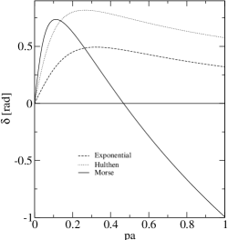
Figure 1: Phase-shift (L=0) for different potentials vs. momentum in inverse range units.

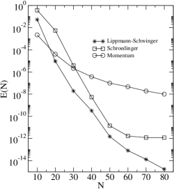
Figure 2: Average relative error (185) for the phase-shift versus $N$ (exponential potential).

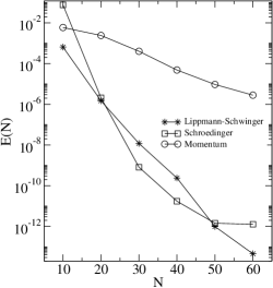
Figure 3: Average relative error (185) for the phase-shift versus $N$ (Hulthén potential).

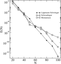
Figure 4: Average relative error (185) for the phase-shift versus $N$ (Morse potential).

Figure 5: Scattering length in inverse range units vs. $s$ for different potentials.

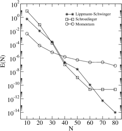
Figure 6: Average relative error (186) for the scattering length versus $N$ (exponential potential).

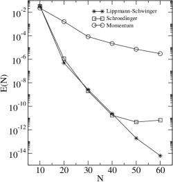
Figure 7: Average relative error (186) for the scattering length versus $N$ (Hulthén potential).

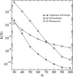
Figure 8: Average relative error (186) for the scattering length versus $N$ (Morse potential).

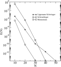
Figure 9: Relative error for the calculated binding energy – exponential potential.

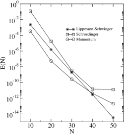
Figure 10: Relative error for the calculated binding energy – Hulthén potential.

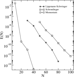
Figure 11: Relative error for the calculated binding energy – Morse potential.

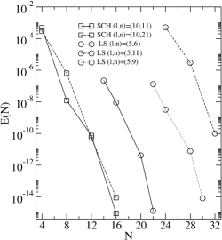
Figure 12: Relative error for the calculated binding energies – Coulomb potential.

In the discrete spectrum problem the dimensionless quantity of interest is the imaginary part of the momentum (in inverse range units) at which the T-matrix has a pole. This, necessarily non-negative quantity, will be denoted as $x(s)$ where we have emphasised its dependence upon the potential strength $s$. Thus, similarly as for the scattering length $A(s)$, a function of $s$ needs to be determined but it is much harder to obtain the exact solution. The function $x(s)$ is known explicitly for the Hulthén potential but (cf. Appendix) for the exponential and the Morse potential $x(s)$ is provided in an entangled form, as a solution of a transcendental equation of the form $F(x,s)=0$ where the function $F$ might be quite complicated. In general, such equation can be solved only numerically and this is a difficult task especially when machine accuracy is desired. Nevertheless, for the exponential potential for some particular $x$ values, $s(x)$ can be obtained quite easily and one such obvious instance is $x=\textstyle\frac{1}{4}$ in which case we get $s=(\pi/2)^{2}$ as the exact solution. Unfortunately, for the Morse potential there is only the hard way left. For testing purposes of the semi-spectral method as the benchmark solutions we used the exact values $s=(\pi/2)^{2},\;x=\textstyle\frac{1}{4}$ for exponential potential and, respectively, $s=3/2,\;x=1$ for the Hulthén potential. For the Morse potential the benchmark solution was obtained numerically. The shape was adopted from darewychgreen where Morse potential was used as a model of proton-neutron interaction in the deuteron (with $a=0.3408\,fm$ and $d=0.8668\,fm$). We slightly retouched the depth so that the potential better reproduces the deuteron binding energy $B=-2.22\,MeV$ and at the pole, we have $s=0.33509414149514,\;x=0.0078864302204068$. The above pairs of values of $(s,x)$ for different potentials were regarded as exact for testing purposes of the semi-spectral method. Using the $s$ value as input, the values of $x$ was subsequently determined by solving the Schrödinger equation, and the L-S equation in the coordinate and in momentum space, respectively. The relative error for $x$ is presented in Figs. 10-12 as a function of the approximation order $N$. Unexpectedly, a comparison of the results obtained by different methods in Figs. 2-12 shows that the unpopular Volterra equation method appears to be the winner.

Finally, in Fig. 12 we display the relative errors for the calculated binding energies in a hydrogen-like system where a point-like charge Coulomb potential was operative. The values of the quantum numbers $(n,\,\ell)$ are given on the plot. We wish to note that in the momentum space calculation there was no need to invoke Lande’s subtraction technique and the difficulty connected with the Coulomb singularity was avoided by using the dedicated weights $\Omega_{j}(z)$, as explained in detail in Sec. VII. Therefore, the results presented in Fig. 12 indirectly involve also a test on the accuracy of the method applied for calculating the singular integrals.

We have been displaying the logarithm of the error versus $N$ as this is convenient for a quick assessment of the asymptotic convergence rate and a linear plot would indicate a geometric convergence (as a reminder we note that an algebraic convergence would lead to a linear dependence between $\log(E)$ and $\log(N)$). It has to be kept in mind, however, that with $N\leq 100$, as adopted in our computations, the approximation order $N$ cannot be really regarded as asymptotic ($N\to\infty$) and a more complicated dependence upon $N$ should not be surprising. Nevertheless, as might have been expected, the semi-spectral errors presented in this Section decrease very rapidly to zero, in most cases showing indeed a geometric convergence.

IX Summary and conclusions

The purpose of this work was a concise presentation of the mathematical techniques associated with the Chebyshev pseudo-spectral method. The emphasis was on the practical aspects in the efficient implementation of this method on high-performance computers, in a manner accessible to newcomers to the field. The paper is self-contained, i.e. apart from a standard linear algebra package, no other resources are needed and the supplied algorithms can be immediately turned into a suite of computer codes capable of solving a wide variety of practical problems. Formal considerations have been illustrated by providing concrete solutions of some typical quantum mechanical problems.

In our experience the pseudo-spectral Chebyshev method seems to be without downsides: the implementation and programing could not have been simpler, the precision and stability are excellent with the convergence being usually exponential. Although the resulting matrices are not sparse but it does not matter since their sizes are not large. Finally, the same scheme can be used for solving differential, integral or integro-differential equations.

Appendix A Configuration space

Denoting the range as $a$ and the depth as $V_{0}$, we introduce two dimensionless quantities: the potential strength parameter $s=2\mu\,V_{0}\,a^{2}$ and the momentum in inverse range units $\xi=pa$. The s-wave phase shift $\delta(s,\xi)$ is a function of $s$ and $\xi$ and the scattering length in the units of range $A(s)/a$ is defined as the limit of $\delta(s,\xi)/\xi$ when $\xi\to 0$.

1. Exponential potential.

   $$2\mu\,V(r)=-(s/a^{2})\,\textstyle{\rm e}^{\displaystyle-r/a}$$

   and only the attractive case will be considered $s\geq 0$. The phase shift, is

   $$\delta(s,\xi)=\Im\ln\left[J_{2\textstyle{\rm i}\xi}(2\sqrt{s})\,\Gamma(1+2\textstyle{\rm i}\xi)\right]-\xi\,\ln s$$

   where $J_{\nu}(x)$ denotes a complex order $\nu$ Bessel function of the first kind. The scattering length, is

   $$A(s)/a=-2(\gamma+\log\sqrt{s})+\pi\,Y_{0}(2\sqrt{s})/J_{0}(2\sqrt{s}),$$

   where $\gamma$ is Euler constant and $Y_{0}(x)$ is the zero-order Bessel function of the second kind. For an assigned value of $s$, the bound states poles are at $\xi=\textstyle{\rm i}\,x$ and are obtained by solving the transcendental equation

   $$J_{2x}(2\sqrt{s})=0$$

2. Hulthén potential.

   $$2\mu\,V(r)=-(s/a^{2})\,\left(\textstyle{\rm e}^{\displaystyle r/a}-1\right)^{-1}$$

   and only the attractive case will be considered $s\geq 0$. The phase shift, is

   $$\delta(s,\xi)=\Im\left[\ln\Gamma(1+2\textstyle{\rm i}\xi)+\ln\Gamma(\sqrt{s-\xi^{2}}-\textstyle{\rm i}\xi)+\ln\Gamma(-\sqrt{s-\xi^{2}}-\textstyle{\rm i}\xi)\right]$$

   and the scattering length, is

   $$A(s)/a=2\gamma-\psi(1+\sqrt{s})-\psi(1-\sqrt{s}),$$

   where $\psi$ denotes the digamma function. The bound state poles occur at $\xi=\textstyle{\rm i}x$ where

   $$x=(s-n^{2})/(2n),\quad n=1,2,3\dots$$

3. Morse potential and Morse barrier.
   In both cases the potential is given by the same expression

   $$2\mu\,V(r)=-(s/a^{2})\,\textstyle{\rm e}^{\displaystyle(d-r)/a}\left[2-\textstyle{\rm e}^{\displaystyle(d-r)/a}\right]$$

   where $d$ is a parameter of the dimension of length. For Morse potential we have $s>0$, whereas $s<0$ for Morse barrier. The phase shift, is

   $$\delta(s,\xi)=\begin{cases}\arg M(\textstyle\frac{1}{2}+\textstyle{\rm i}\displaystyle\xi-\sqrt{s},\,1+2\textstyle{\rm i}\xi,\,z),&\quad s>0\\ \arg\,M(\textstyle\frac{1}{2}+\textstyle{\rm i}\displaystyle\xi-\textstyle{\rm i}\sqrt{-s},\,1+2\textstyle{\rm i}\xi,\,\textstyle{\rm i}\,z)-\textstyle\frac{1}{2}\,z,&\quad s\leq 0\end{cases}$$

   where $z=2\textstyle{\rm e}^{\displaystyle d/a}\,\sqrt{|s|}$ and $M(a,b,z)$ denotes the Kummer function abramowitz . The scattering length, takes the form

   $$A(s)/a=-2\gamma-\psi(\textstyle\frac{1}{2}-\sqrt{s})-\log z-\Gamma(\textstyle\frac{1}{2}-\sqrt{s})\;U(\textstyle\frac{1}{2}-\sqrt{s},\,1,\,z)/M(\textstyle\frac{1}{2}-\sqrt{s},\,1,\,z)$$

   for $s>0$ and

   $$A(s)/a=-2\gamma-\Re\left\{\psi(\textstyle\frac{1}{2}-\textstyle{\rm i}\sqrt{-s})-\log\textstyle{\rm i}z+\Gamma(\textstyle\frac{1}{2}-\textstyle{\rm i}\sqrt{-s})\;U(\textstyle\frac{1}{2}-\textstyle{\rm i}\sqrt{-s},\,1,\,\textstyle{\rm i}z)/M(\textstyle\frac{1}{2}-\textstyle{\rm i}\sqrt{-s},\,1,\,\textstyle{\rm i}z)\right\}$$

   for $s\leq 0$ where $U(a,b,z)$ denotes the Tricomi hypergeometric function abramowitz . For assigned values of $s$ and $d/a$, the bound state poles are at $\xi=\textstyle{\rm i}x$ where $x$ is a solutions of the equation

   $$M(\textstyle\frac{1}{2}+x-\sqrt{s},\,1+2x,\,z)=0,\quad s>0$$

   $$\Re M(\textstyle\frac{1}{2}+x-\textstyle{\rm i}\sqrt{-s},\,1+2x,\,\textstyle{\rm i}z)=0,\quad s<0.$$

4. Coulomb potential.
   For a Coulomb potential of the form $V(r)=-\alpha/r$ where $\alpha$ is the fine structure constant, we have

   $$2\mu\,V(r)=-(2/a^{2})\,(a/r)$$

   where $a=1/\mu\alpha$ is the Bohr radius and only the attractive case will be considered. The phase shift, is

   $$\delta_{\ell}(\xi)=\arg\Gamma(\ell+1-\textstyle{\rm i}/\xi).$$

   Bound states occur at $\xi=\textstyle{\rm i}\,x$ where

   $$x=1/(n+\ell+1),\quad n=0,1,2,\dots.$$

   When a $Z$ factor multiplies the Coulomb potential, as result of scaling $r\to r/Z$ we get $x\to Z\,x$.

Appendix B Momentum space

The potentials in momentum space are obtained from (128). Introducing the abbreviations $x=a(k+k^{\prime}),\;y=a(k-k^{\prime})$, we have

1. Exponential potential:

   $$U_{0}(k,k^{\prime})=-2sa/[(1+x^{2})(1+y^{2})],$$

2. Hulthén potential:

   $$U_{0}(k,k^{\prime})=-2sa\;\dfrac{\Re\psi(1+\textstyle{\rm i}\,x)-\Re\psi(1+\textstyle{\rm i}\,y)}{x^{2}-y^{2}}=-2sa\;\sum_{n=1}^{\infty}\dfrac{n}{(n^{2}+x^{2})(n^{2}+y^{2})},$$

3. Morse potential and Morse barrier:

   $$U_{0}(k,k^{\prime})=-sa\;\dfrac{4\,\textstyle{\rm e}^{d/a}}{(1+x^{2})(1+y^{2})}+sa\;\dfrac{1}{4}\;\dfrac{\textstyle{\rm e}^{2d/a}}{[1+(\textstyle\frac{1}{2}x)^{2}][1+(\textstyle\frac{1}{2}y)^{2}]},$$

4. Coulomb potential:

   $$U_{\ell}(k,k^{\prime})=-4a\;Q_{\ell}(z)/(x^{2}-y^{2})$$

   where $z=(x^{2}+y^{2})/(x^{2}-y^{2})$. Following abramowitz , $Q_{\ell}(z)$ denotes the Legendre function of the second kind which exhibits a logarithmic singularity

   $$Q_{\ell}(z)=P_{\ell}(z)\;\textstyle\frac{1}{2}\log\dfrac{1+z}{1-z}-W_{\ell-1}(z)$$

   with $W_{-1}(z)\equiv 0$ and

   $$W_{\ell-1}(z)=\displaystyle\sum_{n=1}^{\ell}\frac{1}{n}P_{n-1}(z)\,P_{\ell-n}(z),$$

   where $P_{\ell}(z)$ denotes the Legendre polynomial.

References

- (1) B. Fornberg, A practical guide to pseudospectral methods (Cambridge University Press, Cambridge, 1998)
- (2) J.P. Boyd, Chebyshev and Fourier spectral methods (Dover, New York 2001).
- (3) Tao Pang, An Introduction to Computational Physics, (Cambridge University Press, Cambridge 1997)
- (4) M. Abramowitz and I. Stegun, (Eds.), Handbook of Mathematical Functions (Dover, New York 1972).
- (5) P.M. Morse and H. Feshbach, Methods of Theoretical Physics (McGraw Hill, New York 1953)
- (6) P.M. Morse, Phys. Rev. 34, 57 (1929)
- (7) G. Rawitscher, C. Merow, M. Nguyen and I. Simbotin, Am. J. Phys. 70, 935 (2002)
- (8) G. Darewych and A.E.S. Green, Phys. Rev. 164, 1324 (1967)
- (9) L. Hulthén, Ark. Mat. Astron. Fys. A 28, 5 (1942); B 29, 1 (1942)
- (10) B. Durand and L. Durand, Phys. Rev. D 23, 1092 (1981)
- (11) W. van Dijk, Phys. Rev. C 40, 1437 (1989)
- (12) C.S. Lam and Y. P. Varshni, Phys. Status Solidi B 89, 103 (1978)
- (13) J.A. Olson and D.A. Micha, J. Chem. Phys. 68, 4352 (1978)
- (14) S. Flüge, Practical Quantum Mechanics, (Springer, New York, 1974).
- (15) W.H. Press, S.A. Teukolsky, W.T. Vetterling and B.P. Flannery Numerical Recipes (Cambridge University Press, Cambridge, 2002).
- (16) J.C. Mason and D.C. Handscomb, Chebyshev Polynomials (Chapman and Hall, 2002).
- (17) T.J. Rivlin, Chebyshev Polynomials, From Approximation Theory to Algebra and Number Theory, 2nd Edition (Wiley, New York 1990).
- (18) C.W. Clenshaw and A.R. Curtis, Numer. Math. 2, 197(1991).
- (19) S.E. El-gendi, Comput. J. 12, 282 (1969)
- (20) B. Mihaila and I. Mihaila, J. Phys. A: Math. Gen. 35, 731 (2002)
- (21) I.H. Sloan and W.E. Smith, Numer. Math. 30, 415 (1978).
- (22) T. Hasegawa and T. Torii, Math. Comput. 56, 741 (1991).
- (23) R. Omnes, Nuovo Cimento 8, 316 (1958).
- (24) H. Liu, Ch. Elster and W. Gloeckle, Phys. Rev. C 72, 054003 (2005).
- (25) G.F. Drukarev, Zhur. Exp. i Teoret. Fiz. 25, 139 (1953).
- (26) H. Brysk, J. Math. Phys. 4, 1536 (1963).
- (27) R.A. Gonzales, J. Eisert, I. Koltracht, M. Neumann and G. Rawitscher, J. Comput. Phys. 134, 134 (1997)
- (28) S.Y. Kang, I. Koltracht and G. Rawitscher, Math. Compu. 72, 729 (2003)
- (29) S.Y. Kang, J. Comp. App. Math. 169, 277 (2004); Comp. Math. App. 48, 1425 (2004)
- (30) E. Lambert, Helv. Phys. Acta 42, 677 (1969)
- (31) C.J. Noble and I.J. Thompson, Comput. Phys. Commun. 33, (1984) 413.
- (32) C.J. Noble, Comput. Phys. Commun. 159, (2004) 55.
- (33) P. Koval and S. Fritzsche, Comput. Phys. Commun. 172, (2005) 187.
- (34) Yong Rae Kwon and F. Tabakin, Phys. Rev. C18, 932 (1978)
- (35) D.P. Heddle, Yong Rae Kwon and F. Tabakin, Comput. Phys. Commun. 38, 71 (1985)