The limits of counterfactual computation

Abstract

We show that the protocol recently proposed by Hosten et al. Hosten does not allow all possible results of a computation to be obtained counterfactually, as was claimed. It only gives a counterfactual outcome for one of the computer outputs. However, we confirm the observation Hosten that the protocol gives some protection against decoherence. In some situations, though, it may be more effective simply to run the computer several times.

In their recent paper Hosten , Hosten et al. proposed a novel protocol, using the ‘chained Zeno’ principle. This, it was argued, would allow all possible results of a quantum computation to be obtained, with probability close to 1, without running the computer. There is, however, a limit to the information that can be obtained from such a counterfactual computation. Consider a computation with two outputs, 0 and 1, and let $p_{i}$ denote the probability of inferring the result $i$ from a protocol without running the computer, for $i=0\mbox{ or }1$. It was shown in MitJozsa , that $p_{0}+p_{1}\leq 1$. In defiance of this limit, the chained Zeno protocol would allow $p_{0}+p_{1}$ to be arbitrarily close to 2 (in the case of a computation with two possible outputs). The explanation for this contradiction is that the protocol is not fully counterfactual, and it is instructive to see why this is so.

The chained Zeno protocol.

We summarise the protocol, using the notation in the Supplementary Material Hosten . We consider a simplified computation where there are only two outputs, 0 or 1. In other words, we consider only two possible outputs rather than the four in their Grover search example.

The protocol consists of a subroutine inside a routine. When the subroutine runs, the computer can be activated if a switch qubit, the ‘computer switch’, is on (0=off, 1=on). We shall speak of an ‘insertion of the computer’ to mean a step of the subroutine where the computer is activated if its switch qubit is on. There is a second qubit, the ‘subroutine switch’, that controls whether the subroutine is entered from the routine. Finally, there is a third qubit that receives the output of the computation. The entire state can be written $|\Psi\rangle=\sum\alpha_{ijk}|ijk\rangle$, with

$$|ijk\rangle=|\mbox{subroutine switch=i}\rangle|\mbox{computer switch=j}\rangle|\mbox{computer output=k}\rangle.$$

Initially, $|\Psi\rangle=|000\rangle$.

Both the routine and the subroutine use the quantum Zeno principle Misra . At each step, the subroutine applies a rotation $R=\left(\begin{array}[]{cc}\cos\theta&-\sin\theta\\ \sin\theta&\cos\theta\\ \end{array}\right)$ (in the computational basis) to the the computer switch, inserts the computer, then measures the output qubit. There are $N$ steps in the subroutine, with $N\theta=\pi/2$. The routine applies a rotation $R^{\prime}$ by an angle $\theta^{\prime}$ to the subroutine switch, lets the subroutine run, then measures the computer switch. There are $N^{\prime}$ steps in the routine, with $N^{\prime}\theta^{\prime}=\pi/2$.

After the first step of the routine, the rotation $R^{\prime}$, the state is $|\Psi\rangle=\cos\theta^{\prime}|000\rangle+\sin\theta^{\prime}|100\rangle$. Next, the subroutine is switched on in the second term (but not in the first, where the subroutine switch is 0). After the first step of the subroutine, the state is

$$|\Psi\rangle=\cos\theta^{\prime}|000\rangle+\sin\theta^{\prime}\underbrace{\left(\cos\theta|100\rangle+\sin\theta|110\rangle\right)}_{subroutine}.$$ (1)

The brace here indicates the terms that change during the subroutine. Next the computer is inserted, and runs in the second term within the brace, where the computer switch is 1.

To see how the protocol works, we consider the two outputs separately:

Output 0

When the computer runs, equation (1) is unchanged. This happens at every step of the subroutine, which rotates to the final state

$$|\Psi\rangle=\cos\theta^{\prime}|000\rangle+\sin\theta^{\prime}|110\rangle.$$ (2)

The next step in the routine is to measure the computer switch, and this kills the second term with probability close to 1 if $\theta^{\prime}$ is small. Thus we reach the state $|\Psi_{0}\rangle=|000\rangle$, which is also the final state of the routine.

Output 1

When the computer runs, the second term in the brace becomes $\sin\theta|111\rangle$. With probability close to 1, this term is killed when the output qubit is measured. At the end of the subroutine, after $N$ steps, we have the (unnormalised) state $\cos\theta^{\prime}|000\rangle+\sin\theta^{\prime}\cos^{N}\theta|100\rangle$, and, if $N$ is large enough, and hence $\theta$ small enough, this is close to $\cos\theta^{\prime}|000\rangle+\sin\theta^{\prime}|100\rangle$. Measurement of the computer switch qubit does not change this state, and the remaining steps of the routine rotate the state fully, with probability close to 1, to the state $|\Psi_{1}\rangle=|100\rangle$. This state is orthogonal to $|\Psi_{0}\rangle$; the two final states can be distinguished, with probability close to 1, by measuring the subroutine switch qubit at the end of the protocol.

Counterfactuality

We now address the question of whether the computer runs during the protocol. To make this precise, we keep track of whether the computer has run by making a list of the possible sequences of measurement outcomes that can occur, including in each list hypothetical measurements of the computer switch qubit at the end of each insertion of the computer. We call such a list a ‘history’ MitJozsa . Each history $h$ is a list of measurement outcomes (real and hypothetical), which correspond to a product of projectors $P_{1}\cdots P_{k}$; we associate to $h$ the un-normalised vector $v_{h}=P_{1}\cdots P_{k}|000\rangle$. As convenient notation, we write $0_{i}$/$1_{i}$ for the outcome 0/1 of a measurement on the $i$-th qubit in the state, and $f$/$n$ for an ‘off’/‘on’ outcome of the hypothetical measurement of the computer switch. The history is then a list of outcomes and $f$ or $n$ symbols, written left to right in the order of the protocol steps. Tables 2 and 2 show the histories and their associated vectors for one step of the routine, i.e. for the first complete cycle of the subroutine followed by the computer switch measurement. Here we take $N=2$.

Table 1: Histories after one subroutine cycle, with $N=2$. Output 0.

$h$	$v_{h}$
$f0_{3}f0_{3}0_{2}$	$\cos\theta^{\prime}|000\rangle+\sin\theta^{\prime}|100\rangle/2$
$f0_{3}n0_{3}1_{2}$	$\sin\theta^{\prime}|110\rangle/2$
$n0_{3}f0_{3}0_{2}$	$-\sin\theta^{\prime}|100\rangle/2$
$n0_{3}n0_{3}1_{2}$	$\sin\theta^{\prime}|110\rangle/2$

Table 2: Histories for output 1

$h$	$v_{h}$
$f0_{3}f0_{3}0_{2}$	$\cos\theta^{\prime}|000\rangle+\sin\theta^{\prime}|100\rangle/2$
$f0_{3}n1_{3}1_{2}$	$\sin\theta^{\prime}|111\rangle/2$
$n1_{3}f1_{3}0_{2}$	$-\sin\theta^{\prime}|101\rangle/2$
$n1_{3}n1_{3}1_{2}$	$\sin\theta^{\prime}|111\rangle/2$

If $m$ is a particular set of outcomes of the (actual) measurements during the protocol, the histories containing $m$ are added coherently to give the amplitude for $m$. Thus $|x|^{2}$ is the probability of the outcomes $m$, where $x=\sum_{m\subset h}v_{h}$. We are now ready to define a counterfactual computation:

A set $m$ of measurement outcomes is a counterfactual outcome if (1) there is only one history associated to $m$ and that history contains only $f$’s, and (2) there is only a single possible computer output associated to $m$.

Looking at table 2 for the output 1, we see that condition (1) is satisfied for $m=0_{3}0_{3}0_{2}$ which occurs only in the history $h=f0_{3}f0_{3}0_{2}$. This is only a segment of a complete history, covering only one step of the routine. But condition (1) also holds for the complete set of measurement outcomes, and, as the final subroutine switch measurement distinguishes $\Psi_{0}$ from $\Psi_{1}$, condition (2) is satisfied. Thus $m$ is a counterfactual outcome for the output 1.

The situation is different for output 0. Table 2 shows that there are two histories containing $m=0_{3}0_{3}0_{2}$, namely $f0_{3}f0_{3}0_{2}$ and $n0_{3}f0_{3}0_{2}$. Since the latter contains an ‘n’, condition (1) is not satisfied, and there is non-vanishing amplitude for the computer running when the set of measurement outcomes $m$ is obtained. This is therefore not a counterfactual outcome for the output 0. Another way of seeing this is to note that the first term in the brace in equation (1), $\cos\theta|100\rangle$, is removed during the subroutine by destructive interference from terms where the computer runs; this occurs when we add $v_{f0_{3}f0_{3}0_{2}}$ and $v_{n0_{3}f0_{3}0_{2}}$ in Table 2. Thus, for output 0, the final state can only be reached if the computer has run during the protocol.

Now let us consider the whole protocol, and let $m_{i}$ denote the result of the final measurement of the protocol, with $m_{0}=0_{1}$, $m_{1}=1_{1}$. Let $m$ denote the set of measurement results that must be obtained up to that point for the protocol to succeed, i.e. a sequence of $N$ $0_{3}$’s followed by an $0_{2}$ for each run of the subroutine. Then, for instance, $P(mm_{i}|i)$ denotes the probability of the protocol being successful and giving the outcomes appropriate to output $i$ given that the actual computer output is $i$.

Let us define the counterfactuality of outcome $i$ by $c_{i}=|v_{h^{i}}|^{2}$, where $h^{i}$ is the all-$f$ history for outcome $mm_{i}$. Table 5 gives the counterfactualities for a choice of $N$, $N^{\prime}$ satisfying the condition $N\gg N^{\prime}$ for the protocol to run effectively Hosten . The table also shows the probabilities $P(mm_{i}|i)$. For a counterfactual outcome, we expect $c_{i}=P(mm_{i}|i)$, since, by condition (1), only the all-$f$ history contributes to the outcome $mm_{i}$. For output 1, we do indeed have $c_{1}=P(mm_{1}|1)$. However, for output 0, $c_{0}\ll P(mm_{0}|0)$, and we can infer that the outcome is far from counterfactual, since histories in which the computer runs make the dominant contribution to the measurement results.

Decoherence

Suppose now that there is decoherence during the running of the computer (but not during other parts of the protocol), and suppose decoherence makes the computer act according to the admittedly somewhat artificial rule:

$$|11x\rangle|e\rangle\to(1-\epsilon)|11x\rangle|e\rangle+\sqrt{2\epsilon-\epsilon^{2}}|11(1-x)\rangle|e^{\prime}\rangle,$$ (3)

where the computer output $x$ is 0 or 1, and $|e\rangle$ and $|e^{\prime}\rangle$ are environmental states, assumed to be orthogonal, and where $|e^{\prime}\rangle$ is a different state for each computer run.

Table 5 shows the effect of decoherence with $\epsilon=0.2$. The protocol used was not the chained Zeno protocol described above, but a modification of it where the computer is inserted twice in each step of the subroutine ; this works efficiently over a wider range of values of $N$ and $N^{\prime}$. The table shows $P(m|i)$, the probability of the protocol succeeding given computer output $i$, and $P(m_{i}|mi)$, the probability of getting the final measurement result appropriate to the computer output, given that the protocol has been successful. Note that these probabilities increase as the relevant counterfactuality increases. In fact, the values of $N$ and $N^{\prime}$ chosen by Hosten et al. lie in the range where the counterfactualities are approximately equal, as are the relevant probabilities, and it is in this region that one gets the best performance on both computer outputs.

There is therefore an intriguing hint of a connection between counterfactuality and decoherence-resistance. We should bear in mind, however, that the modified chained Zeno protocol inserts the computer $2NN^{\prime}$ times, and time must be allowed on each insertion for the computer to run or not run. We might therefore wish to compare the protocol with the simpler procedure of just running the computer $2NN^{\prime}$ times. Table 5 shows the mutual information gained by the chained Zeno protocol and by $2NN^{\prime}$ repeated runs of the computer, and the latter wins except in the special circumstance of a decoherence so large that the correct and incorrect answers have roughly equal probabilities. Repeated runs then give little information, whereas the interference of terms in the protocol can distinguish between differing states of the environment.

The conclusion seems to be that the benefits of counterfactual computation are limited, although special cases such as interaction-free measurement Elitzur may nevertheless offer some genuine practical utility.

Table 3: ‘Counterfactuality’.

$N$	$N^{\prime}$	$c_{0}$	$c_{1}$	$P(mm_{0}|0)$	$P(mm_{1}|1)$
700	70	0.0015	0.884	0.965	0.884

Table 4: The modified algorithm of Hosten , with $\epsilon=0.2$.

$N$	$N^{\prime}$	$c_{0}$	$c_{1}$	$P(m|0)$	$P(m_{0}|m,0)$	$P(m|1)$	$P(m_{1}|m,1)$
700	70	0.0015	0.884	0.609	0.040	0.973	0.9999
40	70	0.188	0.175	0.625	0.975	0.630	0.969
40	700	0.803	0.0042	0.948	0.9998	0.469	0.107

Table 5: Mutual information for two protocols.

$N$	$N^{\prime}$	$\epsilon$	MI(Chained Zeno)	MI(Repeated runs)
10	10	0.2	0.46	0.9999
2	2	0.2	0.324	0.360
10	10	$1-\sqrt{2}/2$	0.297	0

 

Reply to the Response of Drs Hosten et al.

In their response to us, Hosten et al. Hosten2 propose a new definition of counterfactual computation. A key feature of this new definition is that, if a set of histories have amplitudes that sum to zero, then those histories can be discounted, and are not used in assessing whether the computer runs. For instance, histories 1 and 2 in their Figure 2 have equal and opposite amplitudes and can therefore be discounted.

This discounting rule seems very odd to us. In the classic two-slit experiment, a dark fringe at a point P on the screen arises because the amplitudes for a photon reaching P from the two slits sum to zero. The usual view is that the photon goes through both slits to reach P; their rule seems to imply that the photon goes through neither slit on the way to P. Indeed, we can regard the two slits as being analogous to the two arms of the interferometer in their Figure 2, and it is only by arguing that the photon goes through neither arm that they can claim that the computer C does not run.

We can highlight what is wrong with their new definition by adding a fourth quantum register in their protocol that is initially set to $|0\rangle$ and is incremented every time the computer runs. If the computation is counterfactual, the computer never runs and therefore the fourth register should always be zero. This is the case when the computer output is 1, which we all agree is a counterfactual outcome.

Now consider what happens when the computer output is 0. In place of their Table-I we get our Table 6, and the amplitudes for histories 1 and 2 no longer cancel. The protocol is therefore not counterfactual according to their definition. But if it were counterfactual without the fourth register, it should remain so with this register added.

We conclude that the proposed new definition of counterfactual computation is flawed, and we see no reason to depart from our own definition.

Table 6:

history	$h$	$v_{h}$
1	$n^{(1)}n^{(2)}0_{3}n^{(1)}f^{(2)}0_{3}0_{2}$	$-\sin\theta^{\prime}|1001\rangle/2$
2	$n^{(1)}f^{(2)}0_{3}n^{(1)}f^{(2)}0_{3}0_{2}$	$\sin\theta^{\prime}|1000\rangle/2$
3	$f^{(1)}f^{(2)}0_{3}f^{(1)}f^{(2)}0_{3}0_{2}$	$\cos\theta^{\prime}|0000\rangle$

Reply to further comments of Drs Hosten et al.

In our Reply above, we introduced the idea of a fourth register that counts the number of times the computer runs, and noted that the chained Zeno protocol would not work with this register added. Hosten et al. are quite right to point out, in their Reply Hosten2 , that certain protocols we propose Jozsa99 ; MitJozsa would also not work with this fourth register added. In fact, our definition of a counterfactual computer output $r$ comprises two parts: the first involves the protocol with computer $U_{r}$ (in which $U_{r}$ “does not run”) and the second involves the protocol with computer $U_{1-r}$ (in which the computer is allowed to run). The fourth register above spoils only the second part and not the first.

As a refinement of the fourth register idea, we can test the two possible computer outputs individually. For instance, we can increment the fourth register only when the output is 1, leaving it unchanged for output 0. Then our protocol and the chained-Zeno protocol both function correctly for the output 1, which is counterfactual. As we explained, that is what one expects, since the computer never runs and the fourth register should therefore never change. But if one tests the output 0 in this way on the chained-Zeno protocol, the cancellation does not occur and the protocol fails. Yet it should not fail if 0 were truly a counterfactual output.

We can state this more generally. Let us define a tally register to be a quantum register that keeps a record in some way of whether the computer runs when it has some specified output. It seems reasonable to require, as a general property of counterfactual computation, that adding a tally register for a counterfactual output should not affect the protocol.

This will always be true according to our definition of a counterfactual computation. By contrast, if we use the definition of Hosten et al., then whenever histories with cancelling amplitudes are neglected there will be a tally register that makes the protocol fail. This tally register is incremented in a way that depends on the stage of the algorithm so that distinct histories have distinct final entries in the register (this was why we talked about “incrementing” rather than flipping a bit). Clearly, if the computer runs in any of the cancelled histories, cancellation no longer occurs and the protocol fails. If the computer does not run in any of these histories, it satisfies our definition and the cancellation was unnecessary.

In the Appendix of Hosten2 , Hosten et al. argue that our definition of counterfactuality is inconsistent. First they recall a protocol originally defined in Jozsa99 . Here the first qubit is the computer switch and the second receives the computer output. Define $U$ by $U|0\rangle_{1}|0\rangle_{2}=|0+1\rangle_{1}|0\rangle_{2}/\sqrt{2}$, $U|1\rangle_{1}|0\rangle_{2}=|1-0\rangle_{1}|0\rangle_{2}/\sqrt{2}$ and $U|i\rangle_{1}|1\rangle_{2}=|i\rangle_{1}|1\rangle_{2}$, for $i=0,1$. (Here we are using the shorthand $|0\pm 1\rangle$ for $|0\rangle\pm|1\rangle$). Then the protocol for the case where the computer output is 1 is as follows:

$$|0\rangle_{1}|0\rangle_{2}\ \ \underrightarrow{U}\ \ |0+1\rangle_{1}|0\rangle_{2}/\sqrt{2}\ \ \underrightarrow{computer}\ \ (|0\rangle_{1}|0\rangle_{2}+|1\rangle_{1}|1\rangle_{2})/\sqrt{2}\ \ \underrightarrow{U}\ \ |0+1\rangle_{1}|0\rangle_{2}/2+|1\rangle_{1}|1\rangle_{2}/\sqrt{2}.$$ (4)

If a measurement of the two qubits yields $|0\rangle_{1}|0\rangle_{2}$, this is a counterfactual outcome, according to our definition, because the term does not arise when the computer output is 0, and because the computer switch is never on (the first qubit is never set to $|1\rangle_{1}$) in the terms that give rise to $|0\rangle_{1}|0\rangle_{2}$.

Hosten et al. then propose an internal structure for the computer, replacing it by a Hadamard, followed by a $\pi$ sign-change for the output 1, followed by a second Hadamard. Instead of using the computer switch (the first qubit) to determine whether the computer is on, they use the output qubit, arguing that this can only be set to 1 if the computer runs. The computer step above is then expanded into:

$$\underrightarrow{H}\ \ \frac{|0\rangle|0\rangle}{\sqrt{2}}+\frac{|1\rangle|0+{\tilde{1}}\rangle}{2}\ \ \underrightarrow{\pi}\ \ \frac{|0\rangle|0\rangle}{\sqrt{2}}+\frac{|1\rangle|0-{\tilde{1}}\rangle}{2}\ \ \underrightarrow{H}\ \ \frac{|0\rangle|0\rangle}{\sqrt{2}}+\frac{|1\rangle|0+{1}\rangle}{2\sqrt{2}}-\frac{|1\rangle|\tilde{0}-\tilde{1}\rangle}{2\sqrt{2}},$$ (5)

where a tilde marks terms that belong to a history in which the second qubit has been set to 1 by the first Hadamard. The final operation of $U$ now yields the state:

$$\frac{|0+1\rangle|0\rangle}{2}+\frac{|1-0\rangle|0\rangle}{4}+\frac{|1\rangle|1\rangle}{2\sqrt{2}}-\frac{|\tilde{1}-\tilde{0}\rangle|\tilde{0}\rangle}{4}+\frac{|\tilde{1}\rangle|\tilde{1}\rangle}{2\sqrt{2}},$$

again with the tilde convention. We are not allowed to cancel the terms in $|1-0\rangle|0\rangle$ since they have different histories in terms of the setting of the second qubit. It is clear that, since $|0\rangle|0\rangle$ occurs with a tilde, it is not a counterfactual outcome according to the new definition of this term. This is the supposed inconsistency: this outcome was counterfactual according to our original definition, but with this alternative definition it is no longer counterfactual. However, the rules have changed. We are using a different qubit to assess whether the computer runs, and this new criterion does not infallibly decide between “on” and “off”. It is not surprising that a different question gets a different answer. We take this up again later.

The three-box paradox and weak measurement

Since our last contribution to this discussion, there has been an insightful contribution from L. Vaidman Vaidman , which demonstrates that a particular case of the chained-Zeno protocol is an implementation of the “three-box paradox”. In figure 1, after the photon enters the inner interferometer, its state (labelled by the paths shown in the figure) is $(|A\rangle+|B\rangle+|C\rangle)/\sqrt{3}$. Suppose the computer output is 0. Then, taking into account the phase-reversal $\pi$ and the effects of the two subsequent beam-splitters, one sees that the photon will end up in the detector D if the state is post-selected by $(\langle A|+\langle B|-\langle C|)/\sqrt{3}$. Thus the claim by Hosten et al. that the photon does not pass through the subroutine when the computer output is 0 and detector D fires (see their discussion of their Figure 6) is equivalent to the claim that a photon, initially in state $(|A\rangle+|B\rangle+|C\rangle)/\sqrt{3}$ and post-selected to be in the state $(\langle A|+\langle B|-\langle C|)/\sqrt{3}$, is not in “box B”. The argument in the case of the three-box paradox is that the photon must be in box A because, if it were not, the state would collapse to $(|B\rangle+|C\rangle)/\sqrt{2}$, which has zero amplitude for being post-selected. The paradox is that the same argument can be applied to prove that photon must be in box B, which shows that the reasoning is fallacious.

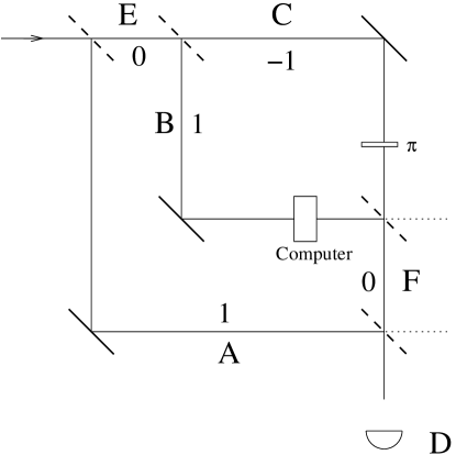
Figure 1: The experiment considered by Vaidman Vaidman , with the labels he assigns to each path and the weak measurement results for the photon being present on various paths in the case where the computer output is 0. The beam-splitters at the top left and bottom right transmit two-thirds of the beam and reflect one-third. Those in the inner interferometer transmit and reflect equally.

Vaidman observed that one can experimentally demonstrate that the photon passes through the computer by carrying out a weak measurement Aharonov98 ; Aharonov01 . A weak measurement of the projection on B, post-conditioned on the photon being detected at D gives the value 1. For C one gets -1, and for F one gets 0. These weak measurement results exactly parallel our argument that the photon must pass through the computer in order for destructive interference to occur at the output of the inner interferometer.

The critique of weak measurement by Hosten et al.

Hosten and Kwiat Hosten-weak have responded to Vaidman’s analysis by questioning the meaning of the weak measurement results shown in Figure 1. First they point out that a weak measurement could be obtained by inserting a tilted parallel glass slab into the path to be measured; this slightly shifts the transverse spatial distribution of the photon and this shift can be read out on path D. If this is done on path B, “there is no longer perfect interference on path F”, and the resulting “leaking amplitude” on path F causes the shift on path D.

We agree with this description. However, they then say that the photons seen in this weak measurement “come from the computer because of the weak measurement”, and the photons are only “weakly present on path B”. Their claim, therefore, is that weak measurement causes photons to pass through the computer, which they would not have done without this measurement taking place. If this is so, what is the block of glass deflecting? A photon that wasn’t there until the block was inserted?

Inconsistency re-examined

We now return to the question of the supposed inconsistency in our definition. The protocol given by the steps (4) gives a counterfactual outcome for the output 1 if we follow our definition and use the computer switch to decide if the computer is on. This is confirmed by weak measurement of the computer switch, which gives the value 0 for the projection onto $|1\rangle_{1}$. However, if we follow Hosten et al. in representing the computer by the sequence of steps (5), and if we deem the computer to be “on” if the output qubit is set to 1, then the outcome is no longer counterfactual. If this is inconsistent, then so are the laws of nature, for if we do a weak measurement of the projection onto $|1\rangle_{2}$ we get the non-zero answer $1/\sqrt{2}$.

The situation is, in fact, closely analogous to that described by Vaidman, who notes that weak measurement of the projections onto both E and F give zero (Figure 1), whereas the weak measurement result for C is 1. As he says: “The photon did not enter the interferometer, the photon never left the interferometer, but it was there!” Vaidman . The interferometer here is the counterpart of Hosten et al.’s internal structure for the computer, interpreting the Hadamards in (5) as the operation of beam-splitters. Their example does not impugn our definition; instead, it affirms that the answer one gets depends on the question one asks.

By contrast, the definition of counterfactuality that Hosten et al. offer does seem to suffer from internal inconsistency, as pointed out by Dr Finkelstein Hosten , because there may be an ambiguity about which histories should be cancelled. They consider an example that corresponds to our Figure 1. There are three histories, following paths B, C and A, that have amplitudes $a$, $-a$ and $a$, respectively (in their Figure 8 they call these histories 1, 2 and 3, respectively). It seems that we could at whim cancel either the first and second of these histories, or the second and third. They argue that the cancellation of B and C happens first in passing through the apparatus, and therefore this is the “correct” cancellation. Thus, they say, the detection of the photon at D must be entirely due to the history through A.

In terms of Vaidman’s three-box analogy, this says that the photon must be in box A. However, as Vaidman observes, one can equally well argue that the photon must be in box B. This makes it clear that their choice is essentially arbitrary. Weak measurements bear this out, because these give $w_{B}=1$, $w_{C}=-1$ and $w_{A}=1$, showing that the ambiguity about cancellation is mirrored in physical data.

Conclusion

Our arguments and Vaidman’s Vaidman lead to the same conclusion: that the chained Zeno algorithm is not counterfactual on all its outputs. Perhaps the most convincing evidence comes from weak measurement. This predicts that, if we select experiments where the photon is detected at D, then a pointer weakly coupled to the path containing the computer will show a deflection (when averaged over many repeats of the experiment). We believe that the argument in Hosten-weak , that this deflection is caused by the weak measurement, is incorrect, and indeed it would be remarkable if a perturbation on a path where no photon was present caused a photon to appear.

It seems to us that the fundamental flaw in their concept of counterfactuality is contained in a sentence in Hosten-weak , where they correctly point out that there is zero amplitude for a photon to travel down path F, but then infer that “a photon does not pass through path B, or the computer, before arriving at path D”. In experiments where a photon is detected at D, there is a non-zero amplitude for it passing along B and a non-zero amplitude for it passing along A, and the fact that there is destructive interference where paths B and C meet does not mean that the amplitude for path B somehow cannot get to the detector and is thereby rendered non-existent. Instead, we have a superposition where the amplitudes for paths A and B both contribute to the detector at D firing. This is beautifully demonstrated by Vaidman’s three-box analogy.

Acknowledgements

We thank Prof. D.J.C. MacKay and Prof. S. Popescu for helpful discussions.

References

- (1) O. Hosten, M. T. Rakher, J. T.Barreiro, N. A. Peters and P. G. Kwiat. Nature, 439: 949-952, (2006).
- (2) B. Misra. J. Math. Phys., 18: 756-763, (1977).
- (3) G. Mitchison and R. Jozsa. Proc. R. Soc. Lond. A, 457: 1175-1193, (2001).
- (4) A. C. Elitzur and L. Vaidman. Found. Phys., 23: 987-997, (1993).
- (5) O. Hosten, M. T. Rakher, J. T.Barreiro, N. A. Peters and P. G. Kwiat. quant-ph/0607101, (2006).
- (6) L. Vaidman. quant-ph/061017, (2006).
- (7) Y. Aharonov, D. Z. Albert and L. Vaidman. Phys. Rev. Lett., 60, 1351, (1998).
- (8) Y. Aharonov, A. Botero, S. Popescu, B. Reznik and J. Tollaksen. quant-ph/0104062 (2001).
- (9) R. Jozsa. Chaos solitons fractals, 10, 1657-1664, (1999).
- (10) O. Hosten and P. G. Kwiat. quant-ph/0612159, (2006).