UWthPh–2006–13 The state space for two qutrits has a phase space structure in its core

Abstract

We investigate the state space of bipartite qutrits. For states which are locally maximally mixed we obtain an analog of the “magic” tetrahedron for bipartite qubits—a magic simplex ${\mathcal{W}}$. This is obtained via the Weyl group which is a kind of “quantization” of classical phase space. We analyze how this simplex ${\mathcal{W}}$ is embedded in the whole state space of two qutrits and discuss symmetries and equivalences inside the simplex ${\mathcal{W}}$. Because we are explicitly able to construct optimal entanglement witnesses we obtain the border between separable and entangled states. With our method we find also the total area of bound entangled states of the parameter subspace under intervestigation. Our considerations can also be applied to higher dimensions.

I Introduction

In 1935 Erwin Schrödinger stated already that “entanglement is the quintessence of the quantum theory”. The late discoveries and developments in many distinct branches of physics show its immense validity. It is the basis for quantum cryptography, quantum teleportation and maybe if realizable quantum computation. It has also triggered a new field: quantum information.

The main problem for composite systems is how to find out if a given state is separable or not and thus to characterize the border between separability and entanglement. While we have for the simplest composite system—two two–level systems ($2\times 2$ systems) or bipartite qubits— a necessary and sufficient criterion for separability, the Peres criterion, it is for higher dimensions only a necessary criterion (except $2\times 3$). The criterion states that every separable density matrix is mapped into a positive semidefinite matrix by partial transposition (PT), i.e., by a transposition on one of the subsystems. The reason why it fails for higher dimensions is that for these systems a completely positive map cannot be characterized by transposition alone and moreover these systems show more aspects of entanglement.

It is obvious that the knowledge of the state space is the key ingredients to understand entanglement and therefore for developing and optimizing new applications. Moreover it will help in understanding the relation of different entanglement measures.

In this paper we focus on bipartite qutrits ($3\times 3$ systems). We concentrate on the set of locally mixed states with a quasiclassical structure and construct a geometrical picture of the state space. The quasiclassical structure fits also exactly into the conditions needed for teleportation and dense coding, e.g. Refs. BW92 ; W01 ; W05 . While these sets of states have been noted already in Ref. VW00 ; N06 , only little is known about its structure concerning entanglement, witnesses, PPT (positive partial transposition) and possible bound entanglement.

For two qubits four orthogonal Bell states can be used to decompose every locally mixed state and a geometric picture can be drawn. In such a geometrical approach the Hilbert-Schmidt metric defines a natural metric on the state space, e.g. Ref. B05 ; Ovrum . Via diagonalizing every locally mixed state can then be described by three real parameters which can be used to identify the density matrix by a point in a $3$–dimensional real space. The positivity condition forms a tetrahedron with the Bell states at the corners and the totally mixed state, the trace state, in the origin. Via reflection one obtains another tetrahedron with reflected Bell states at the corners, see e.g. Ref. BNT02 . The intersection of both simpleces gives an octahedron where all points inside and at the border represent separable states because they are the only ones invariant under reflection and thus positive under PT. While for qubits this characterizes the separable set of locally mixed states fully we show in this paper that the analogue to the octahedron for qutrits is not quite that simple and in addition not all locally maximally mixed states can be imbedded.

The simplex for bipartite qutrits lives in a $9$–dimensional Euclidean space where the borders are given by the positivity condition of density matrices. We construct two polytopes and prove that they are an inner (kernel polytope) and an outer fence (enclosure polytope) to the border of separability. The boundary achieved by taking the set of all states which are positive under PT has not only linear faces and corners but also curved parts. Then we explicitly show how to construct optimal witnesses and apply them to certain states and show that there are regions where there is bound entanglement, i.e. entanglement which cannot be distilled by local operation and classical communication (LOCC).

The paper is organized as follows, we present first the construction of the set of states we are analyzing, the magic simplex ${\mathcal{W}}$. Then we discuss how the set is embedded in the whole set of states. We proceed with analyzing the rich structure of symmetries inside ${\mathcal{W}}$: The symmetry of a discrete classical phase space. Hereupon we focus on describing the boundary of separability by calculating optimal witnesses. The optimization is done analytically and also numerically. Further we added an appendix for more details.

Many of our considerations can be extended to pairs of qudits. In order to be as concrete as possible we postpone generalizations to higher dimensions and more abstract analyzes to a following companion paper.

II The construction of the magic simplex ${\mathcal{W}}$

Throughout this paper we focus on two parties with $3$ degrees of freedom e.g. “qutrits”. Take any maximally entangled pure state vector in the Hilbert space ${\mathbb{C}}^{3}\otimes{\mathbb{C}}^{3}$ for defining a “Bell type state”. Denote this vector as $\Omega_{0,0}$. Choose the bases $\{|0\rangle,|1\rangle,|2\rangle\}$ in each factor such that

$$\Omega_{0,0}=\mbox{$\frac{1}{\sqrt{3}}$}\sum_{s}|s\rangle\otimes|s\rangle\,.$$ (1)

On the first factor in the tensorial product – the side of Alice – we consider actions of the Weyl operators. They are defined by

$$W_{k,\ell}|s\rangle = w^{k(s-\ell)}|s-\ell\rangle,$$ (2)

$$w = e^{2\pi i/3}\,.$$ (3)

Throughout this paper the letters $\{s,t,j,k,\ell,m,n,p,q\}$ denote the numbers $0,1,2$. Calculations with them are to be understood as “modulo 3”. So  “$1+2$”$=0$,  “$2\times 2$”$=1$,  “$-1$”$=2$,  etc.

The transformations which we consider take place on the first factor, on the side of Alice. Bob’s side is in our definitions inert. This is not really an asymmetry. For the Bell state $\Omega_{0,0}$ every action of an operator $A$ on the side of Alice is equivalent to the action of a certain $\tilde{A}$ on the side of Bob. Concerning the Weyl operators the equivalent action is $\tilde{W}_{k,\ell}=w^{-2k\ell}W_{k,-\ell}$. Changing the roles of Alice and Bob i.e. the flip transformation is therefore equivalent to a local reflection combined with a phase factor, but with no change of the total set of the produced states. The phase factors will disappear in the projection operators to be defined in equation (8), and the reflection is one of the symmetries studied in Sect. IV.

The actions of the Weyl operators – we simplify the notation and write $W_{k,\ell}|\Omega\rangle$ meaning $(W_{k,\ell}\otimes{\mathbbm{1}})|\Omega\rangle$ – produce on the whole nine Bell type state vectors

$$\Omega_{k,\ell}=W_{k,\ell}\Omega_{0,0}\,.$$ (4)

The Weyl operators obey the Weyl relations

$$W_{j,\ell}W_{k,m} = w^{k\ell}W_{j+k,\ell+m}\,,$$ (5)

$$W_{k,\ell}^{\dagger}=W_{k,\ell}^{-1} = w^{k\ell}W_{-k,-\ell}\,,$$ (6)

$$W_{0,0} = {\mathbbm{1}}\,.$$ (7)

We remark that the Weyl operators and the unitary group which they form appear sometimes in disguise, under names like “generalized spin operators”, “Pauli group” and “Heisenberg group”, Refs. G98 ; PR04 .

The original use of the Weyl operators, in the chapter “Quantenkinematik als Abelsche Drehungsgruppe” of Ref. W31 was the “quantization” of classical kinematics. (Both continuous and discrete groups have their appearance there.) In the appendix we present a physics model for the bipartite system of qutrits, which may help to visualize the ideas, concerning the interplay of quasiclassical and quantum structures.

The set of index pairs ${(k,\ell)}$ is the discrete classical phase space; $\ell$ denotes the values for the coordinate in “x-space”, $k$ the values of the “momentum”, see also Fig. 1.

To each point in this space is associated a projection operator

$$P_{k,\ell}=|\Omega_{k,\ell}\rangle\langle\Omega_{k,\ell}|\,.$$ (8)

This projection operator is the density matrix for a Bell type state. The mixtures of these pure states form our object of interest, the magic simplex

$${\mathcal{W}}\quad=\quad\{\quad\sum c_{k,\ell}P_{k,\ell}\quad|\quad c_{k,\ell}\geq 0,\quad\sum c_{k,\ell}=1\quad\}\,,$$ (9)

with the nine pure states $P_{k,\ell}$ at the corners. As a geometrical object it is located in an 8-dimensional hyperplane of the 9-dimensional Euclidean space $\{A=\sum a_{k,\ell}P_{k,\ell}\quad|\quad a_{k,\ell}\in{\mathbb{R}}\}$, equipped with a distance relation $\sqrt{{\rm Tr}(A-B)^{2}}$. Specifying the origin $A=0$ in this Euclidean space, it is also equipped with a norm, the Hilbert-Schmidt norm $\sqrt{A^{2}}$, and the inner product ${\rm Tr}(AB)=\sum a_{k,\ell}\,b_{k,\ell}$.

The geometric symmetry of this simplex for the qutrits is larger than the symmetry which is related to the underlying algebraic relations. The later one is equal to the symmetry of the classical phase space. This is studied in Sect. IV.

III How is ${\mathcal{W}}$ embedded in the set of states?

${\mathcal{W}}$ contains only states which are locally maximally mixed, i.e. every partial trace gives the unit matrix times the normalizing constant. Further it contains the maximal possible number of mutually orthogonal pure states. While this characterization is sufficient for qubits, defining the magical tetrahedron or any locally unitary transform of it, this is not so for the qutrits. More explicitly for qubits every locally maximally mixed state can be embedded into a magical tetrahedron, while for the qutrits we observe:

1. There exist locally maximally mixed states, which cannot be diagonalized with maximally entangled pure states, the Bell type states.

2. Even if such a maximally mixed state is decomposable into orthogonal Bell type states, it may be inequivalent to any of the states in ${\mathcal{W}}$.

3. There are maximal sets of nine mutually orthogonal Bell states, which do not build an equivalent of ${\mathcal{W}}$.

Examples are presented in the appendix.

We remark that there are other ways to characterize the density matrices, by expanding them into products of operators which are a basis for the space of matrices. The use of products of Weyl operators in Ref. N06 is closely related to the construction in this paper. And it is the analogue to the use of products of Pauli matrices, e.g. Ref. BNT02 , considered as forming a group. Another method has been tried, considering the analogue of Pauli matrices as generators of $SU(2)$. This leads to using the Gell-Mann matrices, e.g. Ref. B05 , generators of $SU(3)$.

There are several ways how to characterize a special unitary equivalent of one of the versions of ${\mathcal{W}}$. One is already given by the construction: Choose one of the Bell states, and choose some basis on one side. Another way would be a choice of fixed special Bell states which have to be represented. There is a precise statement about the restrictions and the freedom to do this:

THEOREM 1

Every pair of mutually orthogonal Bell states can be embedded into a version of ${\mathcal{W}}$. Such a pair fixes the appearance of a certain third Bell state. A fourth state can then be embedded, if it is orthogonal to the first three. Then, with four different Bell states, all elements of ${\mathcal{W}}$ are fixed.

PROOF Choose one vector out of the pair as $\Omega_{0,0}$. Take a Schmidt decompositions of this vector and of $\Phi$ the second one with the same basis on Bob’s side:

$$\Omega_{0,0}=\mbox{$\frac{1}{\sqrt{3}}$}\sum_{s}|\phi_{s}\rangle\otimes|\eta_{s}\rangle,\quad\Phi=\mbox{$\frac{1}{\sqrt{3}}$}\sum_{s}|\psi_{s}\rangle\otimes|\eta_{s}\rangle.$$

Consider the unitary operator $U=\sum_{s}|\psi_{s}\rangle\langle\phi_{s}|$, acting on the first factor. Orthogonality of the Bell states implies

$$3\,\langle\Omega_{0,0}\,|\,\Phi\rangle={\rm Tr}\,U=0\;.$$

This is possible only if the eigenvalues of U are the three numbers $\{e^{i\delta}w^{k}\}$ with some common phase factor $\delta$. Now let $\{|s\rangle\}$ be the eigenvectors of $U$, and fix $W_{1,0}=e^{-i\delta}U$. This implies $P_{1,0}=|\Phi\rangle\langle\Phi|$. Note, that there are still three phase factors not fixed, one for each basis vector. Nevertheless, the projector $P_{2,0}=W_{1,0}P_{1,0}W_{1,0}^{\dagger}$ is defined unambiguously. The fourth Bell state has a Schmidt decomposition $\mbox{$\frac{1}{\sqrt{3}}$}\sum_{s}|\chi_{s}\rangle\otimes|s\rangle$. Observe that the orthogonality to the first three states implies $\sum_{s}w^{ks}\langle s|\chi_{s}\rangle=0$ for each $k$, and so $\langle s|\chi_{s}\rangle=0$ for each $s$. Together with the orthogonality of the $\chi_{s}$, this implies that either $|\chi_{s}\rangle=e^{i\eta(s)}|s+1\rangle$, or $|\chi_{s}\rangle=e^{i\eta(s)}|s+2\rangle$. Now fix the phases for each $|s\rangle$, such that all $\eta(s)=\eta$, and the fourth Bell state is implemented as either $P_{0,1}$ or as $P_{0,2}$. So all the ingredients for the construction of ${\mathcal{W}}$ are fixed. $\Box$

That the special choice of the positions in the phase space makes no difference for the total set of elements is made clear by consideration of the symmetries inside ${\mathcal{W}}$.

IV Symmetries and equivalences inside ${\mathcal{W}}$

We consider linear symmetry operations mapping ${\mathcal{W}}$ onto itself that can be implemented by local transformations of the Hilbert space. So separability remains unchanged. We show that the transformations of ${\mathcal{W}}$ can be considered as transformations of the quasi classical discrete phase space.

Letting the Weyl operators act on Alice’s side gives the phase space translations:

$$\mathcal{T}_{m,n}:\quad P_{k,l}\mapsto P_{k+m,\ell+n}=W_{m,n}P_{k,\ell}W_{m,n}^{\dagger}\,.$$ (10)

The action is a discrete “Galilei transformation”. The quantization, expressed in the phase factors of the Weyl relations, disappears due to the combined action of $W_{m,n}$ and its adjoint.

In the appendix we present the Weyl operators in matrix form, and also their relations to the phase space. As usual, we take the “x-coordinate” $\ell$ as horizontal and the “momentum coordinate” $k$ as vertical.

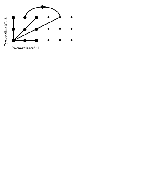
Figure 1: Here we plotted the points $P_{l,k}$ of the discrete classical phase space. $l$ denotes the values of the $x$ coordinate and runs from $0$ to $2$ and $k$ “quantizes” the momentum and runs also from $0$ to $2$. From one fixed point, e.g. $P_{0,0}$, all possible lines are drawn. Thus the phase space can be divided into four bundles where each bundle consists of three parallel lines. In Sect. IV we show that transformations inside the simplex ${\mathcal{W}}$ are equivalent to transformations in this phase space and that the lines are all equivalent in the sense that each line may be transformed into any other one. This enables us to study the geometry of separability in the magic simplex ${\mathcal{W}}$.

For all the other special operations $P_{0,0}$ stays fixed. This is no general restriction, since translations may shift each of the points in phase space to the origin. Now we have to use the help of operators acting on Bob’s side. For every linear operator $A$ on Alice’s side there exists an operator $\tilde{A}$ acting on the other party, such that

$$A|\Omega_{0,0}\rangle=\tilde{A}|\Omega_{0,0}\rangle\,.$$ (11)

They are related through transposition in the preferred basis:

$$\langle s|A|t\rangle=\langle t|\tilde{A}|s\rangle.$$

So, for every local unitary $U$

$$U\tilde{U}^{\dagger}|\Omega_{0,0}\rangle=|\Omega_{0,0}\rangle\,.$$ (12)

Thus every unitary transformation of the Weyl operators can be lifted to a unitary transformation of ${\mathcal{W}}$:

$$W_{m,n} = e^{i\eta}UW_{k,\ell}U^{\dagger},$$ (13)

$$\Rightarrow\qquad P_{m,n} = U\tilde{U}^{\dagger}P_{k,\ell}U^{\dagger}\tilde{U}\,.$$ (14)

This follows in detail from

$$U\tilde{U}^{\dagger}P_{k,\ell}U^{\dagger}\tilde{U} = U\tilde{U}^{\dagger}W_{k,\ell}P_{0,0}W_{k,\ell}^{\dagger}\tilde{U}U^{\dagger}=UW_{k,\ell}\tilde{U}^{\dagger}P_{0,0}\tilde{U}W_{k,\ell}^{\dagger}U^{\dagger}$$ (15)

$$= UW_{k,\ell}U^{\dagger}U\tilde{U}^{\dagger}P_{0,0}U^{\dagger}\tilde{U}UW_{k,\ell}^{\dagger}U^{\dagger}=W_{m,n}P_{0,0}W_{m,n}^{\dagger}\,.$$

First consider

$$U_{R}:\quad|s\rangle\mapsto\mbox{$\frac{1}{\sqrt{3}}$}\sum_{t}w^{-st}\,|t\rangle$$

It effects the quarter rotation of phase space (counter clock-wise)

$$\mathcal{R}:\quad P_{k,\ell}\mapsto P_{\ell,-k}\,.$$ (16)

Then consider

$$U_{V}:\quad|0\rangle\mapsto|0\rangle,\,|1\rangle\mapsto|1\rangle,\,|2\rangle\mapsto w^{2}|2\rangle,$$

it lifts to the vertical shear

$$\mathcal{V}:\quad P_{k,\ell}\mapsto P_{k+\ell,\ell}\,.$$ (17)

Combined action perfects the horizontal shear

$$\mathcal{H}=\mathcal{R}^{-1}\mathcal{V}^{-1}\mathcal{R}:\quad P_{k,\ell}\mapsto P_{k,\ell+k}\,.$$ (18)

Now, for the following reflections we have to consider anti-unitary transformations of the Hilbert space - unless we want to use the flip, the exchange of Alice’s and Bob’s side. The simplest one in our preferred basis is the vertical reflection

$$\mathcal{S}:\quad P_{k,\ell}\mapsto P_{-k,\ell}\,.$$ (19)

It is implemented by complex conjugations

$$\sum_{s}a_{s}|s\rangle\mapsto\sum_{s}a_{s}^{*}|s\rangle$$ (20)

on both factors. Their tensorial product gives global complex conjugation

$$C:\quad\sum_{s,t}a_{s,t}|s\rangle\otimes|t\rangle\mapsto\sum_{s,t}a_{s,t}^{*}|s\rangle\otimes|t\rangle\,.$$ (21)

Obviously

$$C^{-1}=C,\quad CW_{k,\ell}|\Psi\rangle=W_{-k,\ell}C|\Psi\rangle,\quad P_{-k,\ell}=CP_{k,\ell}C.$$

We notice that this anti-unitary transformation is also compatible with the Weyl relations. Since it acts globally, on both factors, it is positivity, separability and PPT preserving. All the structural properties of ${\mathcal{W}}$ which are of interest are symmetric under vertical reflection. Hence they are also symmetric under combined action with other transformations, which give new kinds of reflections, as horizontal reflection

$$\mathcal{R}\mathcal{S}\mathcal{R}^{-1}:\quad P_{k,\ell}\mapsto P_{k,-\ell}$$ (22)

and diagonal reflection

$$\mathcal{R}\mathcal{S}:\quad P_{k,\ell}\mapsto P_{\ell,k}\,.$$ (23)

All the transformations are “linear” or “affine” mappings of the phase space. Phase space lines $((k,\ell),(k+m,\ell+m),(k+2m,\ell+2m))$ are mapped onto lines. Note that the sequence of the three points in a line can be rearranged in any way. With the right relabelling of the indices modulo three one gets again the special prescribed form.

Let us collect our results and state the following theorem:

THEOREM 2

The group of symmetry transformations of ${\mathcal{W}}$ is equal to the group of affine transformations of the quasi classical phase space which is formed by the indices,

$$\left(\begin{array}[]{c}k\\ \ell\end{array}\right)\mapsto\left(\begin{array}[]{cc}m&n\\ p&q\end{array}\right)\left(\begin{array}[]{c}k\\ \ell\end{array}\right)+\left(\begin{array}[]{c}j\\ r\end{array}\right)\,,$$ (24)

where $mq-pn\neq 0$, with all calculations done with integers modulo $3$. For $mq-pn=1$ the transformation of the Hilbert space is unitary, for $mq-pn=-1$ it is anti-unitary.

PROOF Pure phase space translation by $(j,r)$ is the second part, combined with the unit matrix, $m=q=1,\quad n=p=0$. The generating elements for the first part of transformations and the corresponding matrices are (in this Proof we use “$-1$” for “$2$”)

$$\textrm{Quarter rotation:}\qquad\mathcal{R}\quad \leftrightarrow \quad\left(\begin{array}[]{cc}0&1\\ -1&0\end{array}\right),$$ (27)

$$\textrm{Vertical shear:}\qquad\mathcal{V}\quad \leftrightarrow \quad\left(\begin{array}[]{cc}1&1\\ 0&1\end{array}\right),$$ (30)

$$\textrm{Vertical reflection:}\qquad\mathcal{S}\quad \leftrightarrow \quad\left(\begin{array}[]{cc}-1&0\\ 0&1\end{array}\right)\,.$$ (33)

All the invertible matrices can be generated. This can be seen first by looking at the numbers of zeroes. Maximally two zeroes, in relative diagonal positions, are possible, as in $\mathcal{R}$ and $\mathcal{S}$. One zero is possible, as in $\mathcal{V}$. There may be different positions of the zeroes, but they can be moved by the diagonal reflection, applied from the left and/or from the right. The case with no zero in the matrix is represented by $\mathcal{V}\mathcal{H}$. Finally there are different distributions of signs, but they cannot be changed individually, since this would not give invertible matrices. The signs can be changed pairwise, for each column or row, by the vertical reflection $\mathcal{S}$, and by $\mathcal{R}\mathcal{S}\mathcal{R}^{-1}$, applied from the left and/or from the right. $\Box$

The group structure of the combined transformations can be written in matrix notation:

$$\left(\begin{array}[]{c}k\\ \ell\\ 1\end{array}\right)\mapsto\left(\begin{array}[]{ccc}m&n&j\\ p&q&r\\ 0&0&1\end{array}\right)\left(\begin{array}[]{c}k\\ \ell\\ 1\end{array}\right)\,.$$ (34)

The lines in the discrete phase space play also an important role in connection with the Mutually Unbiased Bases, see Refs. PR04 ; W04 ; B04 . In Fig. 1 we visualize all possible lines for one phase space point. Thus we have for the whole phase space four bundles—called “striations” or “pencils” in Refs. W04 ; B04 , respectively—, each one with three parallel lines. This makes 12 special sets out of $\left(\begin{array}[]{c}9\\ 3\end{array}\right)=84$ subsets with three points of the phase space. The lines are all equivalent in the sense that each line may be transformed into any other one. More general, we have

THEOREM 3

In the classes of subsets of phase space points, there is just one equivalence class of single points, one of pairs, two classes of triples and two of quadruples. The equivalence relations are moreover valid also for the complementary sets with five to eight points. Inside each pair and inside each triple, there is total symmetry under permutations.

PROOF We move the subsets to special chosen places in phase space. Consider one point of the subset after the other, in any order. Translation brings the first one to the origin $(0,0)$. The shear transformations bring the second one to $(1,0)$. If these two are part of a line, the third one has then been moved automatically due to the linearity of the transformations, together with the first two, to the point $(2,0)$, completing this vertical line. If the third (or fourth) point is not in a line with the first pair, it is movable with horizontal reflection and vertical shear to the place $(0,1)$, without changing the arrangements of the line with $\ell=0$. In the case of four points, with the vertical line at $\ell=0$ not yet completed, we have several cases: If the fourth point is either at $(2,2)$ or at $(0,2)$, it completes another line, and we can start again, moving this line to the preferred vertical one, and the remaining point as done above. In case the fourth point is not yet at $(1,1)$, where we want to place it, completing a square, it is either at $(2,1)$ or at $(1,2)$, and it can be moved by shear, together with one of the others, to form the preferred square. These are the cases, where no complete line is contained in the subset of four.

The inner symmetries of pairs and triples are now implicitly proven, since the sequence of moving their points can be chosen arbitrarily. $\Box$

V The geometry of separability

We now proceed to the question of separability. We start with a rough analyzes of an inner and outer fence in ${\mathcal{W}}$. Then we concentrate on the border given by PPT. In particular we show that the test for positivity under PT reduces to a check for positivity of a $3\times 3$ matrix. As an example we study the entanglement of mixtures of the total mixed state and two orthogonal Bell type states. We then explicitly describe the construction of witnesses and analyze the strategy to optimize them. We apply our method to the above state and find for some mixtures bound entanglement. As an further example we discuss a density matrix which is a mixture of the total mixed state and three orthogonal Bell states where two of them are equality weighted.

V.1 Two polytopes as inner and outer fences for separability

The most mixed separable state, with density matrix $\omega=\frac{1}{9}{\mathbbm{1}}$, lies at the center of ${\mathcal{W}}$.

$$\omega=\frac{1}{9}\sum_{k,\ell}P_{k,\ell}\,,$$ (35)

since the $\Omega_{k,\ell}$ form an orthonormal basis. The separable states with the largest distance to the center are defined by the lines in the phase space.

THEOREM 4

The twelve outermost separable states in ${\mathcal{W}}$ have the density matrices

$$\rho_{line}=\frac{1}{3}\sum_{(k,\ell)\,\in\,line}P_{k,\ell}\,.$$ (36)

PROOF This is a special case of the more abstract general statement in Ref. N06 equation (36). For a more concrete demonstration, consider the vertical phase space line $\{(k,\ell)\}=\{(0,0),(1,0),(2,0)\}$:

$$P_{k,\ell=0}=\frac{1}{3}\sum_{s,t}w^{k(s-t)}|s,s\rangle\langle t,t|\,,$$ (37)

where we now write $|s,t\rangle$ for $|s\rangle\otimes|t\rangle$. With $\sum_{k}w^{k(s-t)}=3\delta_{s,t}$ one gets

$$\rho_{line}=\frac{1}{3}\sum_{k}P_{k,0}=\frac{1}{3}\sum_{s}|s,s\rangle\langle s,s|\,,$$ (38)

obviously a separable state.

It lies in each one of the three hyperplanes $B_{p,0}$ in our Euclidean space, defined by

$$B_{p,q}=\{(c_{k,\ell})|\,c_{p,q}=\frac{1}{3}\}\,.$$ (39)

$B_{p,0}$ intersects the line of isotropic states $(1-\alpha)\omega+\alpha P_{p,0}$, exactly at the border between separable and entangled states at $\alpha=\frac{1}{4}$, see also Ref. VW00 . This hyperplane is therefore the proper entanglement witness, reduced to our subspace of hermitean matrices. Each state outside is entangled, and it is only the center of the triangle with the $P_{p,0}$ at the corners which is a separable state.

By the equivalence relations stated in Theorem 3, all these considerations are valid for each one of the twelve phase space lines. Now the witness hyperplanes intersect also at the centers of the other 72 ($=84-12$) triangular faces, but the states there are not separable. This is easily checked by showing that they are not PPT. This is done explicitly in the next Sect. V.2. $\Box$

The nine pairs of hyperplanes

$$B_{p,q} = \{(c_{k,\ell})\;|\quad c_{p,q}=\frac{1}{3}\;\}$$ (40)

$$\textrm{and}\qquad A_{p,q} = \{(c_{k,\ell})\;|\quad c_{p,q}=0\;\}$$ (41)

enclose all the separable states of ${\mathcal{W}}$. They define the

$$\textbf{enclosure polytope}\qquad\{(c_{k,\ell})\;|\quad\textrm{all}\;\;c_{p,q}\in[0,\frac{1}{3}]\}\,.$$ (42)

It has the same geometric symmetry as the simplex ${\mathcal{W}}$, which has nine corners. Intersections of the $B_{p,q}$-hyperplanes in triples give 84 vertices. In each of the $B_{p,q}$ there lie 28 of these vertices, the other 56 lie in $A_{p,q}$.

Of these 84 vertices, only twelve are separable states. All the convex combinations of these twelve are again separable states. They form the

$$\textbf{kernel polytope}\qquad\{\rho=\sum_{lines\,\alpha}\lambda_{\alpha}\,\rho_{line\,\alpha}\quad|\quad\lambda_{\alpha}\geq 0,\quad\sum\lambda_{\alpha}=1\}\,.$$ (43)

It has twelve vertices, which are the $\rho_{line}$. Each hyperplane $B_{p,q}$ contains four of them. The other eight are in $A_{p,q}$ and define a full seven-dimensional convex body. This may be compared to the four triangular faces of the qubit-octahedron lying inside the triangles of the magical tetrahedron. The other four, out of all eight, lie in witness planes, see Refs. HH96 ; BNT02 . Here is one more of the many differences between qubits and qutrits (compare with Ref. VW99 ): We do not have the geometric rotation-reflection symmetry between the bordering planes. In the witness-hyperplane $B_{p,q}$ there is only a three-dimensional face (a tetrahedron) with four vertices of the kernel polytope.

That the bordering face in $A_{0,0}$ of the kernel polytope is seven-dimensional can be seen by looking in the Euclidean space of hermitean matrices at the eight vectors $v_{p,q}$, with $(p,q)\neq(0,0)$. Such a vector $v_{p,q}$ is defined as pointing from $\frac{1}{8}({\mathbbm{1}}-P_{0,0})$, the center of the face of ${\mathcal{W}}$ in $A_{0,0}$, to $P_{p,q}$, one of the eight vertices of the seven-dimensional simplicial face of ${\mathcal{W}}$. The center of this face of ${\mathcal{W}}$ is also the center of the eight vertices in $A_{0,0}$ of the kernel polytope. The vector is now representable as a linear combination of the $\rho_{line}$, phase space lines through $(p,q)$ not containing $(0,0)$. By equivalences and symmetries it is sufficient to demonstrate this for one example:

$$2v_{2,2} = -[(P_{1,0}+P_{2,1}+P_{0,2})+(P_{0,1}+P_{1,2}+P_{2,0})]+$$

$$-\frac{1}{3}[(P_{1,0}+P_{1,1}+P_{1,2})+(P_{2,0}+P_{1,1}+P_{0,2})+(P_{0,1}+P_{1,1}+P_{2,1})]+$$

$$+\frac{1}{3}[(P_{2,0}+P_{2,1}+P_{2,2})+(P_{1,0}+P_{0,1}+P_{2,2})+(P_{0,2}+P_{1,2}+P_{2,2})]\,.$$

This consideration is, by equivalence, valid for the maximal face in any $A_{p,q}$.

Every set of phase space points characterizes a face of ${\mathcal{W}}$, with dimension one less than the number $N$ of points. So the types of faces of the kernel polytope, surfacing in a face of ${\mathcal{W}}$, correspond to equivalence classes of sets of phase space points. For $N=7$ there are five vertices $\rho_{line}$, given by the different lines formed by subsets of the $7$ prescribed points. It is not difficult to classify: For $N=6$ there are two types, one type giving faces containing three vertices $\rho_{line}$, the other two. For $N=5$ there are two types, one containing two vertices, the other only one. For $N=4$ either one vertex or none is present; $N=3$ is either a phase space line, giving one vertex at the symmetry center, or another triple with no kernel vertex. Also the edges, $N=2$, contain no vertex.

Note that the facts about isotropic states of qutrits, and the witness hyperplanes $B_{p,q}$ which we use, as above in Theorem 4, is found by us in a new way as a byproduct of our special methods. See the next two Sect. V.2 and Sect. V.3, where we proceed to find out more about the border between the separable and the entangled states.

V.2 PT of our $9\times 9$ matrices

We represent the density matrices in the basis of product vectors

$$|s-\ell,s\rangle=|s-\ell\rangle\otimes|s\rangle$$ (45)

and order them into groups of three, according to $\ell$. Inside each group we order according to $s$. So the global Hilbert space is represented as a direct sum

$${\mathbb{C}}^{3}_{\ell=0}\oplus{\mathbb{C}}^{3}_{\ell=1}\oplus{\mathbb{C}}^{3}_{\ell=2}\,.$$ (46)

The projectors

$$P_{k,\ell}=\frac{1}{3}\sum_{s,t}w^{k(s-t)}|s-\ell,s\rangle\langle t-\ell,t|$$ (47)

do not mix the subspaces. A general matrix of ${\mathcal{W}}$ splits therefore into the direct sum

$$\rho=\sum_{k,\ell}c_{k,\ell}P_{k,\ell}=\left(\sum_{k}c_{k,0}P_{k}\right)\oplus\left(\sum_{k}c_{k,1}P_{k}\right)\oplus\left(\sum_{k}c_{k,2}P_{k}\right)$$ (48)

with the $3\times 3$ matrices

$$P_{0}=\frac{1}{3}\left(\begin{array}[]{ccc}1&1&1\\ 1&1&1\\ 1&1&1\end{array}\right),\quad P_{1}=\frac{1}{3}\left(\begin{array}[]{ccc}1&w^{*}&w\\ w&1&w^{*}\\ w^{*}&w&1\end{array}\right),\quad P_{2}=\frac{1}{3}\left(\begin{array}[]{ccc}1&w&w^{*}\\ w^{*}&1&w\\ w&w^{*}&1\end{array}\right)\,.$$ (49)

Partial transformation is now the linear mapping

$$|s-\ell,s\rangle\langle t-\ell,t|\quad\mapsto\quad|t-\ell,s\rangle\langle s-\ell,t|\quad = \quad|m-s,s\rangle\langle m-t,t|$$ (50)

$$\textrm{with}\qquad m = s+t-\ell\,.$$

It produces a new grouping of the basis vectors $|m-s,s\rangle$, according to $m$, and a new splitting of the global Hilbert space as

$${\mathbb{C}}^{3}_{m=0}\oplus{\mathbb{C}}^{3}_{m=1}\oplus{\mathbb{C}}^{3}_{m=2}\,.$$ (51)

The most general element of ${\mathcal{W}}$ is

$$\rho=A_{\ell=0}\oplus A_{\ell=1}\oplus A_{\ell=2}$$ (52)

with

$$A=\frac{1}{3}\left(\begin{array}[]{ccc}d&a^{*}&a\\ a&d&a^{*}\\ a^{*}&a&d\end{array}\right),\quad d_{\ell}=\sum_{k}c_{k,\ell},\quad a_{\ell}=\sum_{k}w^{k}c_{k,\ell}\,.$$ (53)

Partial transposition maps, as is demonstrated in the appendix, such a matrix $\rho$ into

$$B\oplus B\oplus B,\qquad B=\frac{1}{3}\left(\begin{array}[]{ccc}d_{0}&a_{2}&a_{1}^{*}\\ a_{2}^{*}&d_{1}&a_{0}\\ a_{1}&a_{0}^{*}&d_{2}\end{array}\right)$$ (54)

with three times the same $3\times 3$ matrix. Thus a test for PPT of $\rho$ reduces to a check for positivity of the matrix $B$.

Now we apply the method and use the Peres criterion Ref. P96 : PPT, the positivity under partial transposition, is a necessary condition for separability. So NPT, non-positivity under partial transposition, implies entanglement. The missing detail in the proof of Theorem 4, that the $72$ triangular faces of ${\mathcal{W}}$ not corresponding to phase space lines contain no separable point, is contained in the following

THEOREM 5

Consider a five dimensional face $F$ of ${\mathcal{W}}$, opposite to a triangular face which contains a separable point. $F$ is spanned by the six Bell type states $P_{k,\ell}$ which are not located on the phase space line giving the separable state in the triangular face. The only entangled states in $F$, including its bordering faces, are two $\rho_{line}$, and the edge joining them.

PROOF By equivalence, we may assume that it is the vertical line with $\ell=2$, which gives the separable state in the triangular face, and which stays empty in $F=\{\rho=\sum_{k}c_{k,0}P_{k,0}+\sum_{k}c_{k,1}P_{k,1}\}$. The face $F$ contains $\rho_{line\,\ell=0}$ and $\rho_{line\,\ell=1}$, and the edge joining them $\{\alpha\rho_{line\,\ell=0}+(1-\alpha)\rho_{line\,\ell=1}\}$.

The general matrix, see (52), in $F$ is $\rho=A_{\ell=0}\oplus A_{\ell=1}\oplus 0$. It is transformed by PT, see (54), to three times

$$B=\frac{1}{3}\left(\begin{array}[]{ccc}d_{0}&0&a_{1}^{*}\\ 0&d_{1}&a_{0}\\ a_{1}&a_{0}^{*}&0\end{array}\right).$$

This is only then positive, if $a_{0}=a_{1}=0$. That, in turn, implies, by (53), $c_{0,0}=c_{1,0}=c_{2,0}=\alpha$, and $c_{0,1}=c_{1,1}=c_{2,1}=1-\alpha$. All other $\rho$ are NPT, hence entangled.

The cases of centers of triangular faces not corresponding to a phase space line are represented by $c_{0,0}=c_{1,0}=c_{0,1}=\frac{1}{3}$, with non-vanishing $a_{0}$ and $a_{1}$.$\Box$

In geometric terms, this theorem is a statement about the $N-1$ dimensional faces of ${\mathcal{W}}$, spanned by $N$ vertices with Bell type states. Up to $N=4$ there appear at most single separable points. For $N=5$ and $N=6$ we have to distinguish the equivalence classes. Already for $N=5$, in the class not contained in a face $F$ treated above, there appear new problems: Around the center, the state with coefficients $c_{0,0}=c_{1,0}=c_{2,0}=c_{0,1}=c_{0,2}=\frac{1}{5}$, there is a full four-dimensional set of states, which are outside the kernel polytope, but PPT. This can be observed by looking at the matrix $B$, obtained by PT of this center. It has the coefficients $d_{0}=\frac{3}{5}$, $a_{0}=0$, $a_{1}=a_{2}=d_{1}=d_{2}=\frac{1}{5}$. These coefficients allow for small variations, without destructing the positivity of $B$.

In the next application, looking into the interior of ${\mathcal{W}}$, we study entanglement of mixtures of two orthogonal Bell type states and $\omega$. Note the generality of this case: We use the methods developed for ${\mathcal{W}}$, but, as it follows from our Theorem 1, we can choose any pair of mutually orthogonal Bell states, without reference to any special version of ${\mathcal{W}}$. To apply our methods, we represent the state as

$$\rho=\frac{1-(\alpha+\beta)}{9}{\mathbbm{1}}+\alpha P_{1,0}+\beta P_{2,0},\qquad\textrm{with}\quad\{1+8\alpha-8\beta\geq 0,1-\alpha+8\beta\geq 0\}\,.$$ (55)

This gives, besides $a_{1}=a_{2}=0$, the non-vanishing matrix elements

$$d_{0} = \frac{1+2(\alpha+\beta)}{3}$$

$$d_{1}=d_{2} = \frac{1-(\alpha+\beta)}{3}$$

$$a_{0} = -\frac{\alpha+\beta}{2}+i\frac{\sqrt{3}}{2}(\beta-\alpha)\,.$$

Now, $\rho$ is PPT, iff $B\geq 0$

$$\Leftrightarrow\quad 0\leq d_{1}^{2}-|a_{0}|^{2}=\frac{1}{9}\left(1-2(\alpha+\beta)-\frac{5}{4}(\alpha+\beta)^{2}\right)-\frac{3}{4}(\beta-\alpha)^{2}\,.$$ (56)

This describes, when the inequality is replaced by an equality, a nonlinear border between PPT and NPT states. Special points on this border are:

• isotropic states, $\beta=0$, border point at $\alpha=\frac{1}{4}$

• middle line, $\alpha=\beta$, border point at $\alpha+\beta=\frac{2}{5}$

Now, PPT is, for qutrits, no longer sufficient to guarantee separability, see Refs.H96 ; H98 ; Benatti ; “bound entanglement” may occur. So we have to use more specialized methods, to study the faces not covered by the Theorem 5, and to analyze the interior of ${\mathcal{W}}$.

V.3 Constructions of witnesses

An entanglement witness, $EW_{\rho}$, gives a criterion, to show that a certain state with density matrix $\rho$ is not contained in SEP, the set of separable states; see Ref. T01 .

$$\{EW_{\rho}\}=\{K=K^{{\dagger}}\,\,|\,\,\forall\sigma\in\textrm{SEP}:\quad{\rm Tr}(\sigma K)\geq 0,\,{\rm Tr}(\rho K)<0\}\,.$$ (57)

In this paper we are mostly interested in the structure of SEP. It is a convex set, and as such completely characterized by its tangential hyperplanes. The tangents itself are at the border of a larger set of hyperplanes which do not cut SEP. So we extend the meaning of witness and define SW, the set of structural witnesses:

$$SW=\{K=K^{{\dagger}}\neq 0\,\,|\,\,\forall\sigma\in\textrm{SEP}:\quad{\rm Tr}(\sigma K)\geq 0,\ \}\,.$$ (58)

Similarly, we define $TW_{\rho}$, the set of tangential witnesses for a state on the surface of SEP

$$TW_{\rho}=\{K=K^{{\dagger}}\neq 0\,\,|\,\,\forall\sigma\in\textrm{SEP}:\quad{\rm Tr}(\sigma K)\geq 0,\,\,{\rm Tr}(\rho K)=0\}\,.$$ (59)

The set $SW$ is convex and closed. It is also a linear cone: $K\in SW,\,a\geq 0,\,\Rightarrow aK\in SW$. Therefore the bounded set $\{K\in SW,\ {\rm Tr}K^{{\dagger}}K\leq 1\}$ contains all the mathematical information about $SW$; especially, that its boundary, that is $TW$, is closed. Also, that for every $K$ the family $\{\alpha K-(1-\alpha)\omega\}$ has to intersect the boundary at some $TW_{\rho}$. In geometric terms: In each family of parallel hyperplanes, in the Euclidean space of hemitean matrices, there are two tangential planes. Moreover, because of convexity, closedness and boundedness of SEP: For every $K$ in the boundary of $SW$, there exists at least one $\rho\in\textrm{SEP}$, such that $K$ is a $TW_{\rho}$. The boundary of SEP is our object of main interest.

Here we analyze $\textrm{SEP}\cap{\mathcal{W}}$, and the symmetries of ${\mathcal{W}}$ are an important tool. That a symmetry of a state is reflected in symmetries of its witnesses seems intuitively clear, and has been used already, Ref. N06 . We use this correspondence of symmetries in several details, so we formulate it explicitly:

THEOREM 6

Consider a symmetry group ${\mathcal{G}}$, implemented by unitary and/or antiunitary operators $V_{g}$. Suppose that $\rho$ is ${\mathcal{G}}$-invariant, t.i. $\forall g\,\ V_{g}\rho V_{g}^{-1}=\rho$.

1. If $\rho$ is entangled, there exists a ${\mathcal{G}}$-invariant $EW_{\rho}$.

2. If $\rho$ is on the surface of SEP, there exists a ${\mathcal{G}}$-invariant $TW_{\rho}$.

3. The subset of ${\mathcal{G}}$-invariant elements of SEP is completely characterized by the subset of ${\mathcal{G}}$-invariant elements on the surface of SW, which is the set of ${\mathcal{G}}$-invariant $TW_{\rho}$.

4. All the same is true, when SEP is replaced by the set of PPT-states, entanglement by NPT.

PROOF We use the symmetrizing twirl operation, see Ref. VW00 , $K\mapsto\langle K\rangle_{\mathcal{G}}$. Here we use only finite discrete groups, so the Haar-measure is just summation, and

$$\langle K\rangle_{\mathcal{G}}=\frac{1}{|{\mathcal{G}}|}\sum_{g}V_{g}KV_{g}^{-1},$$ (60)

where $|{\mathcal{G}}|$ is the number of elements in ${\mathcal{G}}$. For every invariant $\rho$ we have

$${\rm Tr}(K\rho)={\rm Tr}(K\langle\rho\rangle_{\mathcal{G}})={\rm Tr}(\langle K\rangle_{\mathcal{G}}\,\rho).$$

If $K$ is an $EW_{\rho}$, then also $\langle K\rangle_{\mathcal{G}}$ is an $EW_{\rho}$, proving (1). If $\rho$ is on the surface of SEP, there exists a $TW_{\rho}$, say $K$, such that ${\rm Tr}(K\rho)=0$. Then also $\langle K\rangle_{\mathcal{G}}$ is a $TW_{\rho}$, proving (2). The set SW is convex and spanned by all convex combinations of $TW_{\rho}$. The same is true for the subset of invariant structural witnesses; they are spanned by all convex combinations of invariant tangential witnesses, on the surface. The invariant density matrices form also a closed convex set, of lower dimension. It is completely characterized by its tangential hyperplanes in this lower dimensional space. These are given through the invariant $SW$’s. This proves (3). To prove (4), one observes that the PPT states form a closed convex set, and that the distinction between PPT and NPT is invariant under unitary and antiunitary transformations. $\Box$

For applications using the symmetries inside of ${\mathcal{W}}$, we use later also the phase space reflections, implemented by local antiunitaries. So we had to consider also this kind of group action.

As first application we consider the group of unitaries $U_{k,\ell}=2P_{k,\ell}-1$ and their products. They are reflections, $U_{k,\ell}^{2}={\mathbbm{1}}$. Our object ${\mathcal{W}}$ is pointwise invariant under this group, and its linear span is the largest set with this property. So, to study witnesses characterizing ${\mathcal{W}}$, we have to consider the invariant opterator

$$K=\sum_{k,\ell}\kappa_{k,\ell}P_{k,\ell}\,.$$ (61)

This is sufficient to obtain all facts about the structure of SEP and PPT in ${\mathcal{W}}$. Note: $K$ is an $EW_{\rho}$ for some state, iff at least one $\kappa_{k,\ell}<0$.

Now, once more, we use the “magic” of Bell type states.

THEOREM 7

The operator

$$K=\sum_{k,\ell}\kappa_{k,\ell}P_{k,\ell}$$ (62)

is a structural witness iff $\forall\phi\in{\mathbb{C}}^{3}$ the operator

$$M_{\phi}=\sum_{k,\ell}\kappa_{k,\ell}W_{k,\ell}|\phi\rangle\langle\phi|W_{k,\ell}^{-1}$$ (63)

is not negative.

$K$ is moreover a $TW$ for some $\rho\in{\mathcal{W}}$, iff $\,\exists\phi$, such that $\det M_{\phi}=0$.

PROOF Each separable state is a convex combination of pure product states $|\psi,\eta\rangle\langle\psi,\eta|$. So $K$ is a $SW$, iff

$$\forall\psi,\eta\quad\langle\psi,\eta|K|\psi,\eta\rangle\geq 0.$$

Now we use the definitions defined in Sect. II

$$P_{k,\ell}=\frac{1}{3}\sum_{s,t}W_{k,\ell}|s,s\rangle\langle t,t|W_{k,\ell}^{-1}$$

and calculate

$$\langle\psi,\eta|P_{k,\ell}|\psi,\eta\rangle=$$

$$=\frac{1}{3}\sum_{s,t}\langle\psi|W_{k,\ell}|s\rangle\langle\eta|s\rangle\langle t|\eta\rangle\langle t|W_{k,\ell}^{-1}|\psi\rangle$$

$$=\frac{1}{3}\langle\psi|W_{k,\ell}|\phi\rangle\langle\phi|W_{k,\ell}^{-1}|\psi\rangle,$$

giving

$$\langle\psi,\eta|K|\psi,\eta\rangle=\frac{1}{3}\langle\psi|M_{\phi}|\psi\rangle\,.$$ (64)

Here we defined the vector $\phi\in{\mathbb{C}}^{3}$ as $|\phi\rangle=\sum_{s}\langle\eta|s\rangle|s\rangle$, with the complex conjugated expansion coefficients of $\eta$. What is true for all $\phi$ is then obviously true for all $\eta$, and vice versa.

If $\det M_{\phi}=0$, there exists an eigenvector $\psi$ with eigenvalue $0$. So $K$ is $TW_{\rho}$ for a density matrix we can define explicitly by

$$\rho=\langle|\psi,\eta\rangle\langle\psi,\eta|\rangle_{\mathcal{G}}\,.$$

We use here the group ${\mathcal{G}}$ with the $U_{k,\ell}$ which we used in the first application of Theorem 6, so $\rho\in{\mathcal{W}}$. On the other hand, if $\exists\rho$ such that $K$ is $TW_{\rho}$, one may expand $\rho=\langle|\psi,\eta\rangle\langle\psi,\eta|+\rho_{rest}$, with $\rho_{rest}$ also being separable. Then

$${\rm Tr}K\rho=\frac{1}{3}\langle\psi|M_{\phi}|\psi\rangle+{\rm Tr}K\rho_{rest}=0.$$

Each of the contributions has to vanish; so $\psi$ is an eigenvector of $M_{\phi}$ with eigenvalue $0$, and $\det M_{\phi}=0$. $\Box$

First application of the Theorem 7: The well known optimal $EW$ for a Bell type state. Consider $P_{0,0}$. We use the symmetry of the phase space sub-group where we fix one point, e.g. $(k,\ell)=(0,0)$, and mix all the other phase space points. An invariant witness has to have the form $K=\gamma P_{0,0}+\beta{\mathbbm{1}}$. This gives

$$M_{\phi}=\gamma|\phi\rangle\langle\phi|+3\beta\|\phi\|^{2}{\mathbbm{1}}\,.$$ (65)

We have used the representation of the unit operator on the global Hilbert space as ${\mathbbm{1}}=\sum_{k,\ell}P_{k,\ell}$. This gives then as contribution to $M_{\phi}$ on ${\mathbb{C}}^{3}$ the operator $\sum_{k,\ell}W_{k,\ell}|\phi\rangle\langle\phi|W_{k,\ell}^{-1}$. This operator is invariant under the Weyl group, and its trace is $9\|\phi\|^{2}$. This can only give $3\|\phi\|^{2}{\mathbbm{1}}$, as the contribution to $M_{\phi}$. The eigenvalues of $M_{\phi}$, for normed $\phi$, are $\gamma+3\beta$, $\beta$,$\beta$. So, if $\gamma=-3\beta$, $K$ is the isotropic witness $TW_{\rho}$ for

$$\rho=\frac{1}{4}P_{0,0}+\frac{3}{4}\omega\,.$$ (66)

In this determination of $EW$, the choice of $\phi$ was completely irrelevant. This is connected with the high symmetry of $P_{0,0}$.

In a next application we consider fewer symmetries. We use the same methods as in Sect. IV, in the equations from (11) to (15). Let ${\mathcal{G}}$, implemented by local unitaries or antiunitaries $V_{g}\tilde{V}_{g}^{-1}$, be the invariance group for $\rho$, an element of ${\mathcal{W}}$. Choosing an invariant witness $K$, associated to the set of matrices $M_{\phi}$, then every $M_{\phi}$ is unitarily equivalent to $M_{\chi}$, with $\chi=V_{g}^{-1}\phi$. This is seen by applying $V_{g}\tilde{V}_{g}^{-1}$ from left and its inverse from the right onto $K$ in equation(64), and calculating its action onto the matrix $M_{\phi}$.

For states and their witnesses which are located on a line in phase space, with an eventual part proportional to $\omega$ or ${\mathbbm{1}}$, this brings essential simplification. By equivalence, we may consider the line $\{(0,0)\ldots(2,0)\}$. All the $W_{k,0}$, consequently the $P_{k,0}$, and of course also the unit operator, are invariant under the group of unitaries $\sum_{s}e^{i\delta(s)}|s\rangle\langle s|$. The consequence is, that each $M_{\phi}$ is equivalent to $M_{|\phi|}$ with real valued non negative vector $|\phi|$.

For general witnesses there remain the phase space translations $V_{g}$, combined with $\tilde{V}_{g}$ as local unitary operators. They act onto the Weyl operators by multiplication with phase factors which cancel in the action onto $K$. The consequence for equivalences of $M_{\phi}$ are the symmetries of $\det M_{\phi}$ under cyclic permutation $\phi_{s}\mapsto\phi_{s+1}$, and the discrete phase twirling $\phi_{s}\mapsto w^{s}\phi_{s}$. One knows therefore, that the determinant depends on the $\phi_{s}$ and their conjugates in the form of symmetric polynomials, invariant under the discrete phase twirling. This allows permutation-symmetric sums with contributions from $|\phi_{s}|^{2}$, from $\phi_{0}^{2}\phi_{1}^{*}\phi_{2}^{*}$, etc. But it forbids contributions as $\phi_{s}^{2}$, $\phi_{0}^{2}\phi_{1}\phi_{2}^{*}$ etc.

Combining these results, it is not difficult to calculate the determinants for witnesses located on the phase space line $\ell=0$, mixed with ${\mathbbm{1}}$: Consider

$$K=\lambda\frac{1}{3}{\mathbbm{1}}+\sum_{k}\gamma_{k}P_{k,0}\,,$$ (67)

related, when $\|\phi\|=1$ to the matrices $M_{\phi}=\lambda{\mathbbm{1}}+\sum_{k}\gamma_{k}W_{k,0}|\phi\rangle\langle\phi|W_{k,0}^{-1}$. The matrix is written explicitly in the appendix. The determinant works out as

$$\det M_{\phi}=\lambda^{3} + \|\phi\|^{2}\left(\gamma_{0}+\gamma_{1}+\gamma_{2}\right)\lambda^{2}$$

$$+ 3\left(|\phi_{0}|^{2}|\phi_{1}|^{2}+|\phi_{1}|^{2}|\phi_{2}|^{2}+|\phi_{2}|^{2}|\phi_{0}|^{2}\right)\left(\gamma_{0}\gamma_{1}+\gamma_{1}\gamma_{2}+\gamma_{2}\gamma_{0}\right)\lambda$$

$$+ 27|\phi_{0}|^{2}|\phi_{1}|^{2}|\phi_{2}|^{2}\gamma_{0}\gamma_{1}\gamma_{2}\,.$$

The analysis follows in the next sections.

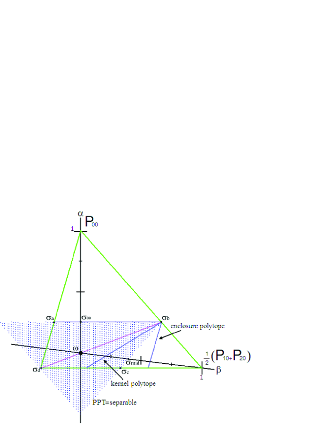
Figure 2: (Color online.) Here the space of the density matrices $\rho=\frac{1-\alpha-\beta}{9}\;\omega+\alpha P_{00}+\frac{\beta}{2}(P_{10}+P_{20})$ is shown. The green triangle shows the positivity condition. The blue lines are the inner fence (kernel polytope) and the outer fence (enclosure polytope) for the boundary of separability. The dotted area shows the values of $\alpha$ and $\beta$ which are positive under PT. Here PPT equals separability.

V.4 Some details in the structure, analytical

The strategy for the exploration of the structure of SEP is to find the set of tangential witnesses as follows: Analyse the operators $K=\sum_{k,\ell}\kappa_{k,\ell}P_{k,\ell}$ by way of studying the set of matrices $M_{\phi}$ associated to each single $K$. If these matrices are positive for all $\phi$, then $K$ is a $SW$. If there is a $\phi$, such that $\det M_{\phi}=0$, then $K$ is a $TW$. If one has “enough” $TW_{\rho}$s, one can determine the $\{\rho\}$ in the boundary of SEP. Consequently, they obey ${\rm Tr}K\rho=0$. How many of these witnesses are “enough”, depends on the symmetry of the subset of states one is studying. High symmetry restricts and simplifies the study.

We study the subset of states with components located on a phase space line, mixed with $\omega$. By equivalence, it is sufficient to study one special line. We choose that with $\ell=0$. The states are $\rho=\alpha\sum_{k}\kappa_{k,0}P_{k,0}+(1-\alpha)\omega$ with $\sum_{k}\kappa_{k,0}=1$. Each of these states is invariant under vertical shear and horizontal reflection. This symmetry group implies that we may restrict the study of witnesses to

$$K=\lambda\frac{1}{3}{\mathbbm{1}}+\sum_{k}\gamma_{k}P_{k,0}\,,$$ (69)

as at the end of Sect. V.3. Note that the parameter $\lambda$ cannot be negative for witnesses, since ${\rm Tr}K\rho_{line\,\ell\neq 0}=\lambda/3$, but ${\rm Tr}K\sigma$ should be non-negative for separable states. And we know already, that all the $\rho_{line}$ are separable, Theorem 4.

Especially simple are those operators, where $\lambda=0$: $K$ is a $TW$, iff all $\gamma_{k}\geq 0$. Because, if all the factors $\gamma_{k}$ are non-zero, then each $M_{\phi}$ is a sum of positive operators. But, if one of them is negative, then, with $\phi=\sum_{s}\frac{1}{\sqrt{3}}|s\rangle$, the matrix $M_{\phi}$ has a negative eigenvalue. Such a $K$ with non-negative $\gamma_{k}$ is no $EW$, but tangential to the face of ${\mathcal{W}}$ spanned by the $P_{k,\ell\neq 0}$.

In the study of the operators with $\lambda>0$, it is enough to consider $\lambda=1$, because the witnesses form a cone, all parameters may be scaled. The investigation, whether $M_{\phi}\geq 0$, is now done by investigation of the characteristic polynomial $\Xi_{c}(\mu)=\det(M_{\phi}-\mu)$. Since $M_{\phi}$ is hermitian, this polynomial, $\Xi_{c}(\mu)=\prod_{j}(\mu_{j}-\mu)$, has only real zeroes $\mu_{j}$. We have to demand that they are not negative, and this is the case if and only if

• the second derivative of $\Xi_{c}$ at $\mu=0$ is not negative,

• The first derivative there is not positive,

• $\Xi_{c}(\mu=0)$ is not negative.

These are conditions for $SW$. To get $TW$, we need one eigenvalue equal to zero, and strengthen the last condition to

• $\Xi_{c}(\mu=0)=0$.

The characteristic polynomial is given by replacing $\lambda$ with $1-\mu$ in the equation (V.3). We use real valued $\phi$ and the abbreviations

$$\begin{array}[]{cccccc}A&:=&\gamma_{0}\gamma_{1}+\gamma_{1}\gamma_{2}+\gamma_{2}\gamma_{0},&\quad\quad B&:=&\gamma_{0}\gamma_{1}\gamma_{2}\\ f_{A}&:=&3(\phi_{0}^{2}\phi_{1}^{2}+\phi_{1}^{2}\phi_{2}^{2}+\phi_{2}^{2}\phi_{0}^{2}),&\quad\quad f_{B}&:=&27\phi_{0}^{2}\phi_{1}^{2}\phi_{2}^{2}\end{array}\,.$$ (72)

The conditions for a tangential witness are given by calculating the derivative $\Xi_{c}$, using $\|\phi\|=1$,

• $3+\sum_{k}\gamma_{k}\geq 0$,

• $3+2\sum_{k}\gamma_{k}+\min_{\phi}(A\cdot f_{A})\geq 0$,

• $1+\sum_{k}\gamma_{k}+\min_{\phi}(A\cdot f_{A}+B\cdot f_{B})=0$.

The minima over normalized wavefunctions $\phi$ are evaluated in the appendix:

$$\min_{\phi}(A\cdot f_{A}) = \min\{0,A\},$$ (73)

$$\min_{\phi}(A\cdot f_{A}+B\cdot f_{B}) = \min\{0,\frac{3}{4}A,\,A+B\}\,.$$ (74)

Because of (73), the first of the conditions as stated above for witnesses is weaker then the second one. And the parameters for $TW$s have to fulfill only one inequality and one equation:

$$3+2\gamma_{0}+4\gamma+\min\{0,A\} \geq 0$$ (75)

$$1+\gamma_{0}+2\gamma+\min\{0,\frac{3}{4}A,\,A+B\} =0\,;$$ (76)

where we use now the parameters

$$\gamma=\frac{1}{2}(\gamma_{1}+\gamma_{2}),\quad\quad\delta=\frac{1}{2}(\gamma_{1}-\gamma_{2})\,.$$ (77)

Using them we get

$$A=2\gamma_{0}\gamma+\gamma^{2}-\delta^{2},\quad\quad A+B=2\gamma_{0}\gamma+\gamma^{2}+\gamma_{0}\gamma^{2}\,.$$ (78)

In the search for $TW_{\rho}$ for $\rho$ symmetric under vertical reflection, i.e. $\kappa_{1,0}=\kappa_{2,0}$, one can restrict the search to operators $K$ which have the same symmetry, that is, they have $\delta=0$. We explore the set of witnesses starting from the isotropic witness, with $\lambda=1$, $\gamma_{0}=-1$, $\gamma=\delta=0$. First we list all those $TW$s one gets, then we indicate the “proof”.

In the set of results we find four distinguished regions for the parameters:

a)

$\lambda=1$,  $\gamma\geq 0$,    $\gamma_{0}=-1$;

b)

$\lambda=1$,  $0\geq\gamma\geq-\frac{2}{3}$, $\gamma_{0}=-1-2\gamma\leq\frac{1}{3}$;

c)

$\lambda=1$,  $\gamma=-\frac{2}{3}$,   $\gamma_{0}\geq\frac{1}{3}$;

d)

$\lambda=0$,  $\gamma\geq 0$,    $\gamma_{0}=1-\gamma>0$.

In the parameter region a) one has $A=\gamma^{2}-2\gamma\geq-1$, so the l.h.s. of Eq. (75) is positive; and $\min\{0,\frac{3}{4}A,A+B\}=-2\gamma$, so Eq. (76) is true. At one end of the region, i.e. in the limit $\gamma\to\infty$, one may rescale the parameters and observe that they approach $\lambda=\gamma_{0}=0$, $\gamma>0$, one end of region d). At the other end of region a), which is also the beginning of region b), the common witness at the edge of these regions is the isotropic witness with $\gamma=0$ and $\gamma_{0}=-1$, corresponding to the hyperplane $B_{0,0}$, defined in Eq. (39) and in Eq. (40). In the parameter region b), succeeding a), neither $A$ nor $A+B$ is negative, since $\gamma\leq 0$, as long as $\gamma\geq-\frac{2}{3}$, with $\gamma_{0}$ related to $\gamma$ by (76). In the succeeding region c) one has $A\leq 0$, and $\frac{3}{4}A\leq A+B$. At the end of this region rescaling leads here, in the limit $\gamma_{0}\rightarrow\infty$, to $\lambda=\gamma=0$, $\gamma_{0}>0$, this is the other end of region d). The round trip is finished.

For regions a), b) and c), we get $EW$s, except for $\gamma=\gamma_{0}=-\frac{1}{3}$ in region b). There we get the $TW_{\rho}$ for all the $\rho$ in the triangular face of ${\mathcal{W}}$ with the $P_{k,0}$ at the vertices.

The linearity of the relations implies, that in each regional set of witnesses each $K$ is a $TW_{\rho}$ for (at least) one common $\rho$. For each $K$ at and endpoint of a region, there exists a linear face of SEP, for which $K$ is tangential .

The vertex points of SEP, corresponding to the linear regions of the witness-parameters, are:

a)

$\sigma_{a}=\omega+\frac{2}{9}P_{0,0}-\frac{1}{9}P_{1,0}-\frac{1}{9}P_{2,0}$;

b)

$\sigma_{b}=\rho_{line\,\ell=0}$;

c)

$\sigma_{c}=\frac{3}{4}(\omega-\frac{1}{9}P_{0,0}+\frac{2}{9}P_{1,0}+\frac{2}{9}P_{2,0})$;

d)

$\sigma_{d}=\frac{3}{2}(\omega-\rho_{line\,\ell=0})=\frac{1}{2}(\rho_{line\,\ell=1}+\rho_{line\,\ell=2})$.

The hyperplane $B_{0,0}$, corresponding to the isotropic witness, contains four $\rho_{line}$, associated with the four phase-space-lines through the phase-space point $P_{0,0}$. One of them is $\sigma_{b}$; the other three have $\sigma_{a}$ in their middle:

$$\sigma_{a}=\frac{1}{3}\left(\frac{1}{3}(P_{0,0}+P_{0,1}+P_{0,2})+\frac{1}{3}(P_{0,0}+P_{1,1}+P_{2,2})+\frac{1}{3}(P_{0,0}+P_{2,1}+P_{1,2})\right).$$

The part of the boundary of SEP between $\sigma_{b}$ and $\sigma_{c}$ is outside the kernel polytope and inside the enclosure polytope. It crosses the ray from $\omega$ to $\frac{1}{2}(P_{1,0}+P_{2,0})$ at $\sigma_{mid}=\frac{1}{5}(3\omega+P_{1,0}+P_{2,0})$.

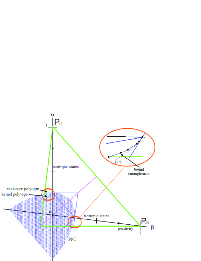
Figure 3: (Color online.) Here the space of the density matrices $\rho=\frac{1-\alpha-\beta}{9}\;\omega+\alpha P_{10}+\beta P_{20}$ is shown. The green triangle shows the positivity condition. The axes joining $\omega$ and $P_{10}$ or $P_{20}$ represent the isotropic states. The blue lines are the inner fence (kernel polytope) and the outer fence (enclosure polytope) for the boundary of separability. The dotted area shows the region of $\alpha$ and $\beta$ where $\rho$ is PPT. For both parameters $\alpha,\beta\geq 0$ PPT gives the boundary between separable and entangled states. For $\alpha$ or $\beta$ negative we find bound entanglement which can be seen in the enlarged picture. The dashed curve shows the border of PPT and for the points the witnesses were explicitly numerically calculated, see Sect. V.5.

V.5 Some details in the structure, numerical

Our method of numerical analysis is a variation of the strategy we use in the previous section. There we calculate first the whole set of tangential witnesses $K$, then we find the $\rho$ on the border of SEP via the condition $Tr(\rho K)=0$. Here we use this condition from the beginning and reduce in this way the set of parameters which have to be varied. We find that explicitly in the following way.

Let us here consider again the density matrix $\rho=\frac{1-\alpha-\beta}{9}\omega+\alpha P_{1,0}+\beta P_{2,0}$ where the state space is visualized in Fig. 3. Via Theorem 7 the operator $K=\mathbbm{1}+aP_{00}+bP_{10}+cP_{20}$ is a structural witness iff the matrix $M_{\phi}=\mathbbm{1}+aW_{0,0}|\phi\rangle\langle\phi|W_{0,0}+bW_{1,0}|\phi\rangle\langle\phi|W_{1,0}+cW_{2,0}|\phi\rangle\langle\phi|W_{2,0}$ is non negative $\forall\phi$. We are moreover interested in the tangential witness, therefore we search for $Tr(\rho K)=0$ which leads to $a=\frac{3+b(1+8\alpha-\beta)+c(1-\alpha+8\beta)}{\alpha+\beta-1}$. Consequently, we have to search for the border where for a given $\alpha$ and the variation over $b,c$ and $\phi$ one eigenvalue of $M_{\phi}$ changes from negative to positive (the two others are positive). The found minimal $\beta$ characterizes then the border state for which a separable state changes to an entangled state, and $K$ is the tangential entanglement witness. We did not include any further symmetry constraints into the calculation and found that the analytical symmetry results as described in the previous section and in the appendix are confirmed, e.g. we have only to vary over real vectors $\phi$. In the region where no bound entanglement was found, the optimized parameter $\beta$ agreed with the PPT calculated $\beta$ numerically up to $10^{-8}$. The largest difference between the PPT boundary and the separability boundary is of the order of $10^{-2}$ and decreases to zero for $\alpha$ or $\beta$ approaching $0$, the isotropic state, see Fig. 3.

VI Summary and conclusions

We consider the state space of two qutrits where we restrict ourselves to locally maximal mixed states. Whereas for qubits every locally maximally mixed state can be diagonalized by the magic Bell states and therefore embedded into a magical tetrahedron, this is not true for qutrits. However, we show that a kind of analogue to the magic tetrahedron can be defined for qutrits: the magical simplex ${\mathcal{W}}$.

Starting from a certain maximally entangled pure state, a Bell type state, we obtain by applying only on Alice side the Weyl operators nine other orthogonal Bell type states. The Weyl operators are used to describe the discrete classical phase space. This discrete classical phase space representing the algebraic relations of the Weyl operators enables us to describe the local transformations of the state space of interest and are very useful for several proofs in this paper. The mixtures of all Bell type states form the simplex ${\mathcal{W}}$ which is then the main object of our investigations.

We show explicitly how to construct a version of ${\mathcal{W}}$. A certain version is fixed by defining $3$ Bell type states. The simplex ${\mathcal{W}}$ can be embedded in a $9$–dimensional Euclidean space equipped with a Hilbert-Schmidt norm and an inner product.

Transformations of ${\mathcal{W}}$ onto itself can be considered as transformations of the discrete classical phase space. Thus the symmetries and equivalences can be studied by this means.

Then we investigate the question of the geometry of separability. We start with constructing two polytopes, an inner (kernel polytope) and an outer (enclosure polytope) fence for separability. They define linear entanglement witnesses but are in general not optimal. The outer fence, the closure polytope, has the same geometric symmetry as ${\mathcal{W}}$.

Hereupon we explicitly study two representative cases. We consider the state space of all density matrices which are mixtures of the total mixed state and two Bell states. We apply the partial positive transformation on one subsystem (PPT) which detects entanglement. The obtained witness is no longer a linear one. We show how entanglement witnesses can be constructed and apply it to the density matrices under consideration. We find after optimizing the entanglement witness by analytical and independently by numerical methods that there is indeed bound entanglement for negative mixtures of one of the Bell states. The result is also visualized in Fig. 3.

The second case we study is the state space of density matrices which are mixtures of the total mixed state, one Bell state and an equal mixture of two other Bell states. We find that it has only linear entanglement witnesses and that no bound entanglement can be found, visualized in Fig. 2.

Summarizing, we could give a full geometric structure of the subset of bipartite qutrits under investigation. We think that this will help to find a good characterization of the whole state space and to investigate measures for entanglement for higher dimensional systems.

VII Appendix

VII.0.1 A physical model

Each party has a system consisting of a ring shaped molecule. In this ring there are three symmetric located possible places for a single itinerant particle. Locating this particle at any of these places corresponds to our three basis vectors $|s\rangle$. In the entangled state, described by the vector $\Omega_{k,\ell}$, the index $\ell$ denotes the angular correlations between Alice’s and Bob’s particles. Concerning measuring of locations, for $\ell=0$ they are to be measured at the places at the same angles. For the two other cases, Alice’s particle is rotated relative to Bob’s. So the number $\ell$ is the quantum number for the observable $s_{Bob}-s_{Alice}$; and the index $k$ is the quantum number for the total angular momentum (component orthogonal to the rings). Again “$-1$”$=2$, due to the finiteness of the system. These two operators commute, while their individual contributions from one party do not; comparable to the commuting of $x_{B}-x_{A}$ with $p_{B}+p_{A}$. The set of their eigenvalue pairs ${(k,\ell)}$ is the discrete classical phase space.

VII.0.2 Examples of maximally mixed states which do not fit into ${\mathcal{W}}$

An example for the observation (1) in Sect. III: Define $\rho=\frac{1}{3}|\Psi\rangle\langle\Psi|+\frac{2}{3}|\Phi\rangle\langle\Phi|$, with $|\Psi\rangle=|0\rangle\otimes|0\rangle$,  and $|\Phi\rangle=\frac{1}{\sqrt{2}}(|1\rangle\otimes|1\rangle+|2\rangle\otimes|2\rangle)$. This density matrix is in a unique way diagonalized, – with non Bell states.

As an example for the observation (2) we consider $\rho=\sum c_{\alpha}|\Psi_{\alpha}\rangle\langle\Psi_{\alpha}|$, with three different orthonomal normalized Bell vectors $\Psi_{\alpha}$ and three different expansion factors $c_{\alpha}$. Since such an expansion is just the expansion into projectors onto eigenvectors, it is unique. So, if $\rho$ can be embedded into ${\mathcal{W}}$ (or a unitary equivalent), the expansion must be an expansion into the $P_{k,\ell}$ (or into a unitarily equivalent set).

Now we give an example of three Bell type projectors which cannot together be embedded into ${\mathcal{W}}$: Take two of the projectors as $P_{0,0}$ and $P_{1,0}$, the third one as $|\Phi\rangle\langle\Phi|$, with $|\Phi\rangle=\mbox{$\frac{1}{\sqrt{3}}$}\sum_{s}w^{2s}\frac{1}{3}(2|s\rangle+2|s-1\rangle-|s+1\rangle)\otimes|s\rangle$. This is a Bell vector, orthogonal to $\Omega_{0,0}$ and $\Omega_{1,0}$. But it is not orthogonal to $\Omega_{2,0}$, so $|\Phi\rangle\langle\Phi|$ cannot be any $P_{k,\ell}$. Now try a transformation and embed the first two projectors as $P_{0,0}=P^{\prime}_{k,\ell}$ and $P_{1,0}=P^{\prime}_{k+m,\ell+n}$ into a unitary equivalent version of ${\mathcal{W}}$. Consider the mapping between these projectors by Weyl operators. As the following equation shows, they are fixed up to a phase

$$P_{1,0}=P^{\prime}_{k+m,\ell+n}=(U\otimes{\mathbbm{1}})P^{\prime}_{k,\ell}(U\otimes{\mathbbm{1}})^{{\dagger}}=(U\otimes{\mathbbm{1}})P_{0,0}(U^{{\dagger}}\otimes{\mathbbm{1}})\,.$$ (79)

Taking the matrix elements with $|s\rangle\otimes|t\rangle$, identifying $U$ with $W^{\prime}_{m,n}$ and comparing with the relation between $P_{0,0}$ and $P_{1,0}$ gives the equations

$$\langle s|W^{\prime}_{m,n}|t\rangle=\langle s|U|t\rangle=e^{i\eta}\langle s|W_{1,0}|t\rangle=e^{i\eta}w^{s}\delta_{s,t}\,.$$ (80)

And this implies, by applying $W^{\prime}_{m,n}$ once more, that $P^{\prime}_{k+2m,\ell+2n}=P_{2,0}$, and the third Bell state does not fit into the equivalent version of ${\mathcal{W}}$ either.

An example for the observation (3): Take the three Bell states $\Omega_{k,2}$ out of ${\mathcal{W}}$ and replace them by

$$\Phi_{k}=\mbox{$\frac{1}{\sqrt{3}}$}\sum_{s}w^{ks}\alpha_{s}|s-\ell\rangle\otimes|s\rangle\,.$$

They are orthogonal, span the same subspace as the deleted $\Omega_{k,2}$, but define other states, unless the phase factors $\alpha_{s}$ are chosen in a very special way. Together with the remaining $\Omega_{k,0}$ and $\Omega_{k,1}$ they form a complete set of orthogonal Bell vectors, but nothing equivalent to ${\mathcal{W}}$.

VII.0.3 Matrices representing the Weyl operators

The basis vectors are

$$|0\rangle=\left(\begin{array}[]{c}1\\ 0\\ 0\end{array}\right),\quad|1\rangle=\left(\begin{array}[]{c}0\\ 1\\ 0\end{array}\right),\quad|2\rangle=\left(\begin{array}[]{c}0\\ 0\\ 1\end{array}\right)\,.$$ (81)

The Weyl operators $W_{k,\ell}$, arranged according to the appearance of the indices in the phase space are

$$\begin{array}[]{ccccccc}k=2&\left(\begin{array}[]{ccc}1&0&0\\ 0&w^{*}&0\\ 0&0&w\end{array}\right),&\left(\begin{array}[]{ccc}0&1&0\\ 0&0&w^{*}\\ w&0&0\end{array}\right),&\left(\begin{array}[]{ccc}0&0&1\\ w^{*}&0&0\\ 0&w&0\end{array}\right),\\ \\ k=1&\left(\begin{array}[]{ccc}1&0&0\\ 0&w&0\\ 0&0&w^{*}\end{array}\right),&\left(\begin{array}[]{ccc}0&1&0\\ 0&0&w\\ w^{*}&0&0\end{array}\right),&\left(\begin{array}[]{ccc}0&0&1\\ w&0&0\\ 0&w^{*}&0\end{array}\right),\\ \\ k=0&\left(\begin{array}[]{ccc}1&0&0\\ 0&1&0\\ 0&0&1\end{array}\right),&\left(\begin{array}[]{ccc}0&1&0\\ 0&0&1\\ 1&0&0\end{array}\right),&\left(\begin{array}[]{ccc}0&0&1\\ 1&0&0\\ 0&1&0\end{array}\right),\\ \\ \quad\ell=&0&1&2\end{array}\,.$$ (116)

Complex conjugation interchanges the lines $k=2$ and $k=1$.

The transformation producing unitary operators are represented as

$$U_{R}=\frac{1}{\sqrt{3}}\left(\begin{array}[]{ccc}1&1&1\\ 1&w^{*}&w\\ 1&w&w^{*}\end{array}\right),\qquad U_{V}=\left(\begin{array}[]{ccc}1&0&0\\ 0&1&0\\ 0&0&w^{*}\end{array}\right)\,.$$ (117)

VII.0.4 The partial transposition

The basis elements are the product vectors $|s-\ell,s\rangle$. They are arranged in groups of three, according to $\ell$. Inside each group the ordering is according to $s$. The index-pairs $(s-\ell,s)$ denoting the rows are written on the left side. Partial transposition induces a new splitting of the Hilbert space in subspaces. They are characterized by $m$, when we write the index-pairs now as $(m-s,s)$. We mark the different $m$ by different typefaces; $\bf{a}$ for $m=0$, $\rm{a}$ for $m=1$, $a$ for $m=2$. (But the numbers are the same, independent of the typeface!)

$$\begin{array}[]{c}(0,0)\\ (1,1)\\ (2,2)\\ \\ (2,0)\\ (0,1)\\ (1,2)\\ \\ (1,0)\\ (2,1)\\ (0,2)\\ \end{array}\quad\left(\begin{array}[]{ccccccccccc}\bf{d_{0}}&\rm{a_{0}^{*}}&a_{0}&&0&0&0&&0&0&0\\ \rm{a_{0}}&d_{0}&\bf{a_{0}^{*}}&&0&0&0&&0&0&0\\ a_{0}^{*}&\bf{a_{0}}&\rm{d_{0}}&&0&0&0&&0&0&0\\ \\ 0&0&0&&d_{1}&\bf{a_{1}^{*}}&\rm{a_{1}}&&0&0&0\\ 0&0&0&&\bf{a_{1}}&\rm{d_{1}}&a_{1}^{*}&&0&0&0\\ 0&0&0&&\rm{a_{1}^{*}}&a_{1}&\bf{d_{1}}&&0&0&0\\ \\ 0&0&0&&0&0&0&&\rm{d_{2}}&a_{2}^{*}&\bf{a_{2}}\\ 0&0&0&&0&0&0&&a_{2}&\bf{d_{2}}&\rm{a_{2}^{*}}\\ 0&0&0&&0&0&0&&\bf{a_{2}^{*}}&\rm{a_{2}}&d_{2}\\ \end{array}\right)\qquad\bf{\mapsto}$$ (140)

$$\begin{array}[]{c}\\ (0,0)\\ (1,1)\\ (2,2)\\ \\ (2,0)\\ (0,1)\\ (1,2)\\ \\ (1,0)\\ (2,1)\\ (0,2)\\ \end{array}\quad\left(\begin{array}[]{ccccccccccc}\bf{d_{0}}&0&0&&0&0&\bf{a_{2}}&&0&\bf{a_{1}^{*}}&0\\ 0&d_{0}&0&&a_{2}&0&0&&0&0&a_{1}^{*}\\ 0&0&\rm{d_{0}}&&0&\rm{a_{2}}&0&&\rm{a_{1}^{*}}&0&0\\ \\ 0&a_{2}^{*}&0&&d_{1}&0&0&&0&0&a_{0}\\ 0&0&\rm{a_{2}^{*}}&&0&\rm{d_{1}}&0&&\rm{a_{0}}&0&0\\ \bf{a_{2}^{*}}&0&0&&0&0&\bf{d_{1}}&&0&\bf{a_{0}}&0\\ \\ 0&0&\rm{a_{1}}&&0&\rm{a_{0}^{*}}&0&&\rm{d_{2}}&0&0\\ \bf{a_{1}}&0&0&&0&0&\bf{a_{0}^{*}}&&0&\bf{d_{2}}&0\\ 0&a_{1}&0&&a_{0}^{*}&0&0&&0&0&d_{2}\\ \end{array}\right)\,.$$ (164)

VII.0.5 The matrix $M_{\phi}$ for witnesses on a line, mixed with the unit

We use real valued $\phi_{s}$. This is possible because of the invariances as described at the end of the Sect. V.3:

$$\left(\begin{array}[]{ccccc}\lambda+\phi_{0}^{2}(\gamma_{0}+\gamma_{1}+\gamma_{2})&&\phi_{0}\phi_{1}(\gamma_{0}+w^{*}\gamma_{1}+w\gamma_{2})&&\phi_{0}\phi_{2}(\gamma_{0}+w\gamma_{1}+w^{*}\gamma_{2})\\ \phi_{1}\phi_{0}(\gamma_{0}+w\gamma_{1}+w^{*}\gamma_{2})&&\lambda+\phi_{1}^{2}(\gamma_{0}+\gamma_{1}+\gamma_{2})&&\phi_{1}\phi_{2}(\gamma_{0}+w^{*}\gamma_{1}+w\gamma_{2})\\ \phi_{2}\phi_{0}(\gamma_{0}+w^{*}\gamma_{1}+w\gamma_{2})&&\phi_{2}\phi_{1}(\gamma_{0}+w\gamma_{1}+w^{*}\gamma_{2})&&\lambda+\phi_{2}^{2}(\gamma_{0}+\gamma_{1}+\gamma_{2})\end{array}\right)\,.$$ (165)

VII.0.6 The minima for the functions of $\phi$, used in Sect. V.4

We use real valued, normalized wavefunctions $\phi$ and describe them with the two parameters

$$z = \phi_{0}^{2}\quad\in[0,1],$$ (166)

$$x = \frac{1}{2}(\phi_{1}^{2}-\phi_{2}^{2})\quad\in[-\frac{1-z}{2},+\frac{1-z}{2}]\,.$$ (167)

The minima of the functions of $\phi$ can be evaluated as minima of functions of $z$ and $x$ in the triangular region determined in (166) and (167). The functions defined in the Sect. V.4 in Eq.(72) are

$$f_{A} = \frac{3}{4}(1+2z-3z^{2})-3x^{2},$$ (168)

$$f_{B} = 27z\left(\frac{(1-z)^{2}}{4}-x^{2}\right)\,.$$ (169)

Because of the terms quadratic in $x$, the extrema are attained either at the boundary of the triangle, or at the line $x=0$. One finds the minimum of $f_{A}$ at the triangle-vertices, equal to $0$. The maximum is attained in the center, at $z=\frac{1}{3}$, equal to $1$. Now one has to respect the sign of $A$:

$$\min_{x,z}(A\cdot f_{A})=\min\{0,A\}\,.$$ (170)

In the combinations of $f_{A}$ with $f_{B}$ also the maximum of $f_{A}$ at the border of the triangle comes into consideration. It is found at the center of a border line and it is equal to $\frac{3}{4}$.

The non negative function $f_{B}$ is zero along the whole boundary and has its maximum, equal to $1$, at the center. The minimum of $Af_{A}+Bf_{B}$ is zero, attained at a vertex, if both $A$ and $B$ are non-negative. It is attained at the center, and equal to $A+B$, if both $A$ and $B$ are non-positive. For different signs of $A$ and $B$ one has to analyse $Af_{A}+Bf_{B}$ along the line $x=0$. Consider

$$f_{A}+Cf_{B}=\frac{3}{4}(1-z)\left(1+3z+9Cz(1-z)\right)$$

as functions of $z$, depending on the parameter $C=B/A$. For every $C$ they have fixed values at $z=0$ – there they are $\frac{3}{4}$ – and at $z=1$ – where they are $0$. For every $C$ the first derivative at $z=\frac{1}{3}$ is zero. There is either a local minimum – if $C<-\frac{1}{3}$ –, a local maximum – if $C>-\frac{1}{3}$ –, or a saddle point. Now we consider the function with special values of the parameter $C$: For $C=-1$, it is zero at $z=1/3$, which is a local minimum. For $C=-1/4$, the local maximum at $z=1/3$ is equal to the maximal value $\frac{3}{4}$ at the border, at $z=0$. Inside the region $0<z<1$ the set of functions is pointwise monotone increasing in the parameter $C$. So for $C$ in between the special values, the minimum is zero, the maximum is $\frac{3}{4}$, both attained at the border. For $C\leq-1$, the minimum, $1+C$, is attained at the center, the maximum, $\frac{3}{4}$, at the border. For $C\geq-\frac{1}{4}$, the minimum, zero, is attained at a vertex, the maximum, $1+C$, at the center.

The result can be stated in a unified way as the equation

$$\min_{x,z}(A\cdot f_{A}+B\cdot f_{B})=\min\{0,\frac{3}{4}A,A+B\}\,.$$ (171)

It means, that the search for the minimum over all $\phi$ can be reduced to considering only three different vectors:

$$\left(\begin{array}[]{c}1\\ 0\\ 0\end{array}\right),\quad\quad\frac{1}{\sqrt{2}}\left(\begin{array}[]{c}1\\ 1\\ 0\end{array}\right),\quad\quad\frac{1}{\sqrt{3}}\left(\begin{array}[]{c}1\\ 1\\ 1\end{array}\right)\,.\quad\quad$$ (172)

References

- (1) C.H. Bennett, S.J. Wiesner: Communication via one- and two-particle operators on Einstein-Podolsky-Rosen state, Phys. Rev. Lett. 69, 2881 – 4 (1992).
- (2) R.F. Werner: All teleportation and dense coding schemes, J. Phys. A 34, 7081 – 94 (2001).
- (3) Shengjun Wu et al.: Deterministic and Unambiguous Dense Coding, arXiv:quant-ph/0512169.
- (4) K. G. H. Vollbrecht, R. F. Werner: Entanglement measures under symmetry, Phys. Rev. A 64, 062307 (2001).
- (5) H. Narnhofer: Entanglement reflected in Wigner Functions, J. Phys. A 39, 7051 – 64.
- (6) R.A. Bertlmann, K. Durstberger, B.C. Hiesmayr and P. Krammer: Optimal Entanglement Witnesses for Qubits and Qutrits, Phys. Rev. A 72, 052331 (2005).
- (7) J.M. Leinaas, J. Myrheim, E. Ovrum, Geometrical aspects of entanglement, arXiv:quant-ph/0605079.
- (8) D. Gottesman in Quantum computing and quantum communications: First NASA International Conference, edited by C.P.Williams (Springer Verlag, Berlin, 1999).
- (9) O. Pittenger, M.H. Rubin: Mutually unbiased bases, generalized spin matrices and separability, Lin. Alg. Appl. 390, 255 – 278 (2004), and references therein.
- (10) H. Weyl: Gruppentheorie und Quantenmechanik, zweite Auflage, (S. Hirzel, Leipzig, 1931).
- (11) R.A. Bertlmann, H. Narnhofer and W. Thirring: Geometric picture of entanglement and Bell inequalities, Phys. Rev. A 66, 032319 (2002).
- (12) W.K. Wootters: Quantum measurements and finite geometry; arXiv:quant-ph/0406032
- (13) I. Bengtsson: MUBs, polytopes and finite geometries; arXiv:quant-ph/0406174
- (14) R. Horodecki, and M. Horodecki: Information-theoretic aspects of inseparability of mixed states, Phys. Rev. A 54, 1838 – 43 (1996).
- (15) K. G. H. Vollbrecht, R.F. Werner: Why Two Qubits Are Special, J. Math Phys. 41, 6772 – 82 (2000).
- (16) A. Peres: Separability Criterion for Density Matrices, Phys. Rev. Lett. 77, 1413 (1996).
- (17) M. Horodecki, P. Horodecki and M. Horodecki: Separability of mixed states: necessary and sufficient conditions, Phys. Lett. A 233, 1 – 8 (1996).
- (18) M. Horodecki, P. Horodecki and R. Horodecki: Mixed-State Entanglement and Distillation: Is there a “Bound” Entanglement in Nature?, Phys. Rev Lett. 80, 5239 – 42 (1998).
- (19) F. Benatti, R. Floreanini and M. Piani: Non-decomposable quantum dynamical semigroups and bound entangled states, Open Syst. Inf. Dyn. 11, 325-338 (2004).
- (20) B.M. Terhal: Detecting Quantum Entanglement, Journal of Theoretical Computer Science 287, 313 – 35 (2002).