Quantum Error Correction via Convex Optimization

Abstract

We show that the problem of designing a quantum information error correcting procedure can be cast as a bi-convex optimization problem, iterating between encoding and recovery, each being a semidefinite program. For a given encoding operator the problem is convex in the recovery operator. For a given method of recovery, the problem is convex in the encoding scheme. This allows us to derive new codes that are locally optimal. We present examples of such codes that can handle errors which are too strong for codes derived by analogy to classical error correction techniques.

1 Introduction

Quantum error correction is essential for the scale-up of quantum information devices. A theory of quantum error correcting codes has been developed, in analogy to classical coding for noisy channels, e.g., [S95, S96, G96, KL97]. Recently [RW05] and [YHT05] did this by posing error correction design as an optimization problem with the design variables being the process matrices associated with the encoding and/or recovery channels. Using fidelity measures leads naturally to a convex optimization problem, specifically a semidefinite program (SDP) [BV04]. The advantage of this approach is that noisy channels which do not satisfy the standard assumptions for perfect correction can be optimized for the best possible encoding and/or recovery.

In [RW05] the power-iteration method was used to find optimal codes for various noisy channels, by alternately optimizing the encoding and recovery channels. In contrast, here we apply convex optimization via SDP, and similarly iterate between encoding and recovery. For a given encoding operator the problem is convex in the recovery. For a given method of recovery, the problem is convex in the encoding. We further make use of Lagrange Duality to alleviate some of the computational burden associated with solving the SDP for the process matrices. The SDP formalism also allows for a robust design by enumerating constraints associated with different error models. We illustrate the approach with an example where the error system does not assume independent channels.

An intriguing prospect is to integrate the results found here within a complete “black-box” error correction scheme, that takes quantum state (or process) tomography as input and iterates until it finds an optimal error correcting encoding and recovery.

2 Quantum Error Correction

2.1 Standard model

A standard model [NC00, §10.3] of an error correction system as shown in the block diagram of Figure 1 is composed of three quantum operations: encoding ${\mathcal{C}}$, error ${\mathcal{E}}$, and recovery ${\cal R}$.

Figure 1: Standard encoding-error-recovery model of an error correction system.

The input, $\rho_{S}$, is the $n_{S}\times n_{S}$ dimensional density matrix which contains the quantum information of interest and which is to be processed. We will refer to $\rho_{S}$ as the system state or the unencoded state. The output of the encoding operation is $\rho_{C}$, the $n_{C}\times n_{C}$ dimensional encoded state. The error operator, which is also the source of decoherence, corrupts the encoded state and returns $\sigma_{C}$, the $n_{C}\times n_{C}$ “noisy” encoded state. Finally, $\rho_{R}$ is the $n_{R}\times n_{R}$ dimensional recovered state. The objective considered here is to design $({\mathcal{C}},{\cal R})$ so that the map $\rho_{S}\to\rho_{R}$ is as close as possible to a desired $n_{S}\times n_{S}$ unitary $L_{S}$. Hence, $\rho_{R}$ has the same dimension as $\rho_{S}$, that is, $n_{R}=n_{S}$. For emphasis we will replace $\rho_{R}$ with $\hat{\rho}_{S}$.

Although it is possible for ${\mathcal{E}}$ to be non-trace preserving, in the model considered here, all three quantum operations are each characterized by a trace-preserving operator-sum-representation (OSR):

$$\begin{array}[]{lll}\displaystyle\rho_{C}={\mathcal{C}}(\rho_{S})=\sum_{c}\ C_{c}\rho_{S}C_{c}^{\dagger},&\displaystyle\sum_{c}\ C_{c}^{\dagger}C_{c}=I_{n_{S}},&\displaystyle C_{c}\in{\mathbf{C}}^{n_{C}\times n_{S}}\\ &&\\ \displaystyle\sigma_{C}={\mathcal{E}}(\rho_{C})=\sum_{e}\ E_{e}\rho_{C}E_{e}^{\dagger},&\displaystyle\sum_{e}\ E_{e}^{\dagger}E_{e}=I_{n_{C}},&\displaystyle E_{e}\in{\mathbf{C}}^{n_{C}\times n_{C}}\\ &&\\ \displaystyle\hat{\rho}_{S}={\cal R}(\sigma_{C})=\sum_{r}\ R_{r}\sigma_{C}R_{r}^{\dagger},&\displaystyle\sum_{r}\ R_{r}^{\dagger}R_{r}=I_{n_{C}},&\displaystyle R_{r}\in{\mathbf{C}}^{n_{S}\times n_{C}}\end{array}$$ (1)

These engender a single trace-preserving quantum operation, ${\cal S}$, mapping $\rho_{S}$ to $\hat{\rho}_{S}$,

$$\begin{array}[]{rcl}\displaystyle\hat{\rho}_{S}&=&\displaystyle{\cal S}(\rho_{S})=\sum_{r,e,c}\ S_{rec}\ \rho_{S}S_{rec}^{\dagger}\\ &&\\ \displaystyle S_{rec}&=&\displaystyle R_{r}E_{e}C_{c}\in{\mathbf{C}}^{n_{S}\times n_{S}}\;\Rightarrow\;\sum_{r,e,c}\ S_{rec}^{\dagger}S_{rec}=I_{n_{S}}\end{array}$$ (2)

Before we describe our design approach we make a few remarks about the error source and implementation of the encoding and recovery operations.

2.2 Implementation

Any OSR can be equivalently expressed, and consequently physically implemented, as a unitary with ancilla states [NC00, §8.23]. An equivalent system-ancilla-bath representation of the standard error correction model of Figure 1 is shown in the block diagram of Figure 2.

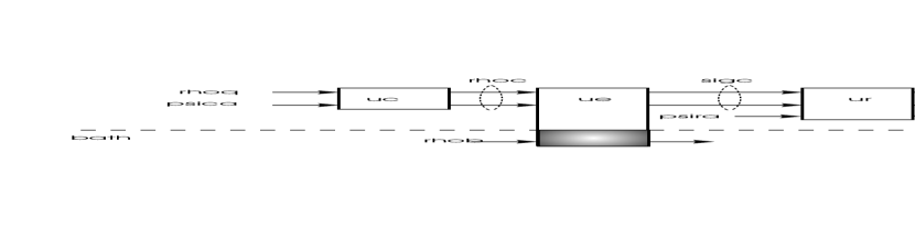
Figure 2: System-ancilla-bath representation of standard encoding-error-recovery model of error correction system.

For the encoding operator, ${\mathcal{C}}$, the encoding ancilla state, $\mbox{\boldmath$|$}0_{CA}\mbox{\boldmath$\rangle$}$, has dimension $n_{CA}$, and hence, the resulting encoded space has dimension $n_{C}=n_{S}\ n_{CA}$. The encoding operation is determined by $U_{C}$, the $n_{C}\times n_{C}$ unitary encoding operator which produces the encoded state $\sigma_{C}=U_{C}(\rho_{S}\otimes\mbox{\boldmath$|$}0_{CA}\mbox{\boldmath$\rangle$}\mbox{\boldmath$\langle$}0_{CA}\mbox{\boldmath$|$})U_{C}^{\dagger}$ .

For the error system, ${\mathcal{E}}$, the ancilla states are engendered by interaction with the environment, or the term used here, the bath. Here we will ignore complications associated with an infinite dimensional bath. The error system is thus equivalent to the $n_{E}\times n_{E}$ unitary error operator $U_{E}$ with uncoupled inputs, $\rho_{C}$ the encoded state, and $\rho_{B}$, the $n_{B}\times n_{B}$ bath state. Thus, $n_{E}=n_{S}n_{CA}n_{B}$. The noisy encoded state $\sigma_{C}$, is the $n_{C}\times n_{C}$ reduced state obtained by tracing out the bath from the output of $U_{E}$, that is, $\sigma_{C}={\bf Tr}_{B}\ U_{E}(\rho_{C}\otimes\rho_{B})U_{E}^{\dagger}$ .

The recovery system ${\cal R}$ has additional ancilla $\mbox{\boldmath$|$}0_{RA}\mbox{\boldmath$\rangle$}$ of dimension $n_{RA}$. $U_{R}$ is the $n_{R}\times n_{R}$ unitary recovery operator with $n_{R}=n_{S}n_{CA}n_{RA}$ and with $\sigma_{R}$ the $n_{R}\times n_{R}$ full output state $\sigma_{R}=U_{R}(\sigma_{C}\otimes\mbox{\boldmath$|$}0_{RA}\mbox{\boldmath$\rangle$}\mbox{\boldmath$\langle$}0_{RA}\mbox{\boldmath$|$})U_{R}^{\dagger}$ . The $n_{S}\times n_{S}$ reduced output state, $\hat{\rho}_{S}$, is given by the partial trace over all the ancillas, the bath having been traced out in the previous step. Specifically, $\hat{\rho}_{S}={\bf Tr}_{A}\ \sigma_{R}$

Caveat emptor

The “real” error correction system is unlikely to be accurately represented by the system shown in Figure 2, but rather by a full system-ancilla-bath interaction [ALZ05]. As shown in the block diagram in Figure 3, $U_{QAB}$ is the $n_{QAB}\times n_{QAB}$ unitary system-ancilla-bath operator, $\mbox{\boldmath$|$}0_{CA}0_{RA}\mbox{\boldmath$\rangle$}$ is the total ancilla state of dimension $n_{CA}n_{RA}$ and $\rho_{B}$ is the bath state. The reduced system output state, $\hat{\rho}_{S}$, is obtained from the full output state $\rho_{QAB}$ by tracing simultaneously over all the ancilla and the bath, $\hat{\rho}_{S}={\bf Tr}_{AB}\ \rho_{QAB}$. At this level of representation, there is no distinction between the $n_{CA}$ ancilla states used for encoding and the $n_{RA}$ ancilla states used for recovery. The internal design, however, may be constructed with such a distinction.

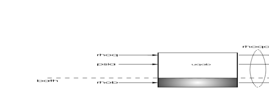
Figure 3: System-ancilla-bath representation of error correction system.

2.3 Optimal error correction: maximizing fidelity

As stated, the goal is to make the operation $\rho_{S}\to\hat{\rho}_{S}$ be as close as possible to a desired unitary operation $L_{S}$. Measures to compare two quantum channels are typically based on fidelity or distance, e.g., [GLN05], [KGBR06]. Let ${\cal S}$ denote a trace-preserving quantum channel mapping $n$-dimensional states to $n$-dimensional states,

$${\cal S}(\rho)=\sum_{k}S_{k}\rho S_{k}^{\dagger},\;\;\;\sum_{k}S_{k}^{\dagger}S_{k}=I_{n}$$ (3)

The following fidelity inequalities hold:

$$f_{\rm mixed}\leq f_{\rm pure}\leq f_{\rm avg}$$ (4)

where

$$\begin{array}[]{rcl}f_{\rm mixed}&=&\min_{\rho}\sum_{k}|{\bf Tr}\ S_{k}\rho|^{2}\\ &&\\ f_{\rm pure}&=&\min_{\mbox{\boldmath$|$}\psi\mbox{\boldmath$\rangle$}}\sum_{k}|\mbox{\boldmath$\langle$}\psi\mbox{\boldmath$|$}S_{k}\mbox{\boldmath$|$}\psi\mbox{\boldmath$\rangle$}|^{2}\\ &&\\ f_{\rm avg}&=&\frac{1}{n^{2}}\sum_{k}|{\bf Tr}S_{k}|^{2}\end{array}$$ (5)

All are in [0,1] and equal to one if and only if ${\cal S}(\rho)=\rho$. From (2), ${\cal S}=L_{S}^{\dagger}{\cal R}{\mathcal{E}}{\mathcal{C}}$ with OSR elements $S_{k}=S_{rec}=L_{S}^{\dagger}R_{r}E_{e}C_{c}\in{\mathbf{C}}^{n_{S}\times n_{S}}$. Thus $f_{\rm avg}=1$ $\Leftrightarrow$ ${\cal S}={\mathcal{I}}_{S}$ $\Leftrightarrow$ ${\cal S}={\cal R}{\mathcal{E}}{\mathcal{C}}=L_{S}$.

Given ${\cal S}$, not all these fidelity measures are easy to calculate. Specifically, $f_{\rm mixed}$ is a convex optimization over all densities, that is, over all $\rho\in{\bf C}^{n\times n},\ \rho\geq 0,\ {\bf Tr}\ \rho=1$, and hence, can be numerically obtained. Calculation of $f_{\rm avg}$ is direct. Calculating $f_{\rm pure}$ is, unfortunately, not a convex optimization over all pure states $\mbox{\boldmath$|$}\psi\mbox{\boldmath$\rangle$}$. If, however, the density associated with $f_{\rm mixed}$ is nearly rank one, then $f_{\rm mixed}\approx f_{\rm pure}$.

As a practical matter, when dealing with small channel errors, it does not matter which fidelity measure is used. Therefore it is convenient to use $f_{\rm avg}$, as it is already in a form explicitly dependent only on the OSR elements. In [RW05] $f_{\rm avg}$ was also used as the design measure, but specific convex optimization algorithms were not proposed. In [YHT05] a similar optimization was proposed using a distance measure to obtain the recovery given the encoding.

We now focus on the optimization problem,

$$\begin{array}[]{ll}\mbox{maximize}&f_{\rm avg}({\cal R},{\mathcal{C}})=\frac{1}{n_{S}^{2}}\sum_{r,e,c}\ \left|{\bf Tr}\ L_{S}^{\dagger}R_{r}E_{e}C_{c}\right|^{2}\\ &\\ \mbox{subject to}&\sum_{r}\ R_{r}^{\dagger}R_{r}=I_{n_{C}},\;\;\;\sum_{r}\ C_{c}^{\dagger}C_{c}=I_{n_{S}}\end{array}$$ (6)

The optimization variables are the OSR elements $\left\{C_{c}\right\}$ and $\left\{R_{r}\right\}$. As posed this is a difficult optimization problem. The objective function is not a convex function of either of the design variables. In addition, the equality constraints are quadratic, and hence, not convex sets. The problem, however, can be approximated using convex relaxation, where each nonconvex constraint is replaced with a less restrictive convex constraint [BV04]. This finally results in a bi-convex optimization problem in the encoding and recovery operator elements which can be iterated to yield a local optimum. As we show next, iterating between the two problems is guaranteed to increase fidelity of each of the relaxed problems. When the iterations converge, all that can be said is that a local solution has been found.

3 Optimal error correction via bi-convex relaxation

3.1 Process matrix problem formulation

Following the procedure used in quantum process tomography [NC00, §8.4.2], [KWR04] we expand each of the OSR elements $R_{r}\in{\mathbf{C}}^{n_{S}\times n_{C}}$ and $C_{c}\in{\mathbf{C}}^{n_{C}\times n_{S}}$ in a set of basis matrices, respectively, for ${\mathbf{C}}^{n_{S}\times n_{C}}$ and ${\mathbf{C}}^{n_{C}\times n_{S}}$, that is,

$$\begin{array}[]{rcl}R_{r}&=&\sum_{i}\ x_{ri}\ B_{Ri}\\ C_{c}&=&\sum_{i}\ x_{ci}\ B_{Ci}\end{array}$$ (7)

where $\left\{\,B_{Ri}\in{\mathbf{C}}^{n_{S}\times n_{C}},\ B_{Ci}\in{\mathbf{C}}^{n_{C}\times n_{S}}\,\left|\,i=1,\ldots,n_{S}n_{C}\,\right.\right\}$ and the $\left\{x_{ri}\right\}$ and $\left\{x_{ci}\right\}$ are complex scalars. Problem (6) can then be equivalently expressed as,

$$\begin{array}[]{ll}\mbox{maximize}&f_{\rm avg}({\cal R},{\mathcal{C}})\equiv f_{\rm avg}(X_{R},X_{C})=\sum_{ijk\ell}\ (X_{R})_{ij}\ (X_{C})_{k\ell}\ F_{ijk\ell}\\ &\\ \mbox{subject to}&\sum_{ij}\ (X_{R})_{ij}\ B_{Ri}^{\dagger}B_{Rj}=I_{n_{C}}\\ &\\ &\sum_{k\ell}\ (X_{C})_{k\ell}\ B_{Ck}^{\dagger}B_{C\ell}=I_{n_{S}}\\ &\\ &(X_{R})_{ij}=\sum_{r}\ x_{ri}x_{rj}^{*}\\ &\\ &(X_{C})_{k\ell}=\sum_{c}\ x_{ck}x_{c\ell}^{*}\\ &\\ &F_{ijk\ell}=\sum_{e}\ ({\bf Tr}\ L_{S}^{\dagger}B_{Ri}E_{e}B_{Ck})({\bf Tr}\ L_{S}^{\dagger}B_{Rj}E_{e}B_{C\ell})^{*}/n_{S}^{2}\end{array}$$ (8)

The optimization variables are the process matrices $X_{R},\ X_{C}\in{\mathbf{C}}^{n_{S}n_{C}\times n_{S}n_{C}}$ and the scalars $\left\{x_{ri}\right\}$ and $\left\{x_{ci}\right\}$. The problem data which describes the desired unitary and error system is contained in the $\left\{F_{ijk\ell}\right\}$. The equality constraints $(X_{R})_{ij}=\sum_{r}\ x_{ri}x_{rj}^{*}$ and $(X_{C})_{k\ell}=\sum_{c}\ x_{ck}x_{c\ell}^{*}$ are both quadratic, exposing again that this is not a convex optimization problem. We do not explore the possible simplifications that can occur in these expressions if the basis matrices are chosen prudently, e.g., ${\bf Tr}\ B_{i}^{\dagger}B_{j}=\delta_{ij}$.

3.2 Design of ${\cal R}$ given ${\mathcal{C}}$ and ${\mathcal{E}}$

In this section and in the remainder of the paper we set the desired logical operation to identity, i.e., $L_{S}=I_{S}$; just error correction not correction and computation. This is without loss of generality as a desired logical operation can be added everywhere.

Suppose the encoding ${\mathcal{C}}$ is given (and $L_{S}=I_{S}$). Then optimizing only over ${\cal R}$ in (8) can be equivalently expressed as,

$$\begin{array}[]{ll}\mbox{maximize}&f_{\rm avg}({\cal R},{\mathcal{C}})\equiv f_{\rm avg}(X_{R},{\mathcal{C}})={\bf Tr}\ X_{R}W_{R}({\mathcal{E}},{\mathcal{C}})\\ &\\ \mbox{subject to}&\sum_{i,j}\ (X_{R})_{ij}\ B_{Ri}^{\dagger}B_{Rj}=I_{n_{C}}\\ &\\ &(X_{R})_{ij}=\sum_{r}\ x_{ri}x_{rj}^{*}\\ &\\ &(W_{R}({\mathcal{E}},{\mathcal{C}}))_{ij}=\sum_{c,k,\ell}\ x_{ck}x_{c\ell}^{*}\ F_{ijk\ell}=\sum_{e,c}\ ({\bf Tr}\ B_{Ri}E_{e}C_{c})({\bf Tr}\ B_{Rj}E_{e}C_{c})^{*}/n_{S}^{2}\end{array}$$ (9)

The optimization variables are the matrix $X_{R}\in{\mathbf{C}}^{n_{S}n_{C}\times n_{S}n_{C}}$ and the scalars $\left\{x_{ri}\right\}$. The problem data is contained in the positive semidefinite matrix $W_{R}({\mathcal{E}},{\mathcal{C}})\in{\mathbf{C}}^{n_{S}n_{C}\times n_{S}n_{C}}$. The objective function is now linear in $X_{R}$, which is of course a convex function. However, each of the equality constraints, $(X_{R})_{ij}=\sum_{r}\ x_{ri}x_{rj}^{*}$ is quadratic, and thus does not form a convex set. This set of quadratic equality constraints can be relaxed to the matrix inequality constraint, $X_{R}\geq 0$, that is, $X_{R}$ is positive semidefinite, a convex set in the elements of $X_{R}$. A convex relaxation of (9) is then,

$$\begin{array}[]{ll}\mbox{maximize}&{\bf Tr}\ X_{R}W_{R}({\mathcal{E}},{\mathcal{C}})\\ &\\ \mbox{subject to}&X_{R}\geq 0,\;\;\;\sum_{i,j}\ (X_{R})_{ij}\ B_{Ri}^{\dagger}B_{Rj}=I_{n_{C}}\end{array}$$ (10)

This class of convex optimization problems is referred to as an SDP, for semidefinite program [BV04]. For a given encoding ${\mathcal{C}}$, the optimal solution to the relaxed problem (10), $X_{R}^{\rm rlx\_opt}$, provides an upper bound on the average fidelity objective in (6) or (8). From the fidelity inequalities (4), we can derive a lower bound. Specifically, the (unknown, possibly unknowable) solution to the original problem (6), is bounded as follows:

$$f_{\rm mixed}({\cal R}^{\rm rlx\_opt},{\mathcal{C}})\leq\max_{{\cal R}}\ f_{\rm pure}({\cal R},{\mathcal{C}})\leq f_{\rm avg}({\cal R}^{\rm rlx\_opt},{\mathcal{C}})={\bf Tr}\ X_{R}^{\rm rlx\_opt}W_{R}S({\mathcal{E}},{\mathcal{C}})$$ (11)

where ${\cal R}^{\rm rlx\_opt}$ is the OSR with elements $\left\{R_{r}^{\rm rlx\_opt}\right\}$ obtained from $X_{R}^{\rm rlx\_opt}$ via the singular value decomposition,

$$X_{R}^{\rm rlx\_opt}=VSV^{\dagger}\;\Rightarrow\;R_{r}^{\rm rlx\_opt}=\sqrt{s_{r}}\ \sum_{i=1}^{n_{S}n_{C}}\ V_{ir}B_{Ri},\;\;r=1,\ldots,n_{S}n_{C}$$ (12)

where $V\in{\mathbf{C}}^{n_{S}n_{C}\times n_{S}n_{C}}$ is unitary and $S={\rm diag}(s_{1}\ \cdots\ s_{n_{S}n_{C}})$ with singular values in decreasing order, $s_{1}\geq s_{2}\geq\ \cdots\ \geq s_{n_{S}n_{C}}\geq 0$.

3.3 Design of ${\mathcal{C}}$ given ${\cal R}$ and ${\mathcal{E}}$

Repeating the previous steps, optimizing only over ${\mathcal{C}}$ in (8) can be equivalently expressed as,

$$\begin{array}[]{ll}\mbox{maximize}&f_{\rm avg}({\cal R},{\mathcal{C}})\equiv f_{\rm avg}(X_{C},{\cal R})={\bf Tr}\ X_{C}W_{C}({\mathcal{E}},{\cal R})\\ &\\ \mbox{subject to}&\sum_{k,\ell}\ (X_{C})_{k\ell}\ B_{Ck}^{\dagger}B_{C\ell}=I_{n_{S}}\\ &\\ &(X_{C})_{k\ell}=\sum_{c}\ x_{ck}x_{c\ell}^{*}\\ &\\ &(W_{C}({\mathcal{E}},{\cal R}))_{k\ell}=\sum_{r,i,j}\ x_{ri}x_{rj}^{*}\ F_{ijk\ell}=\sum_{e,r}\ ({\bf Tr}\ B_{Ck}R_{r}E_{e})({\bf Tr}\ B_{C\ell}R_{r}E_{e})^{*}/n_{S}^{2}\end{array}$$ (13)

The optimization variables are the matrix $X_{C}\in{\mathbf{C}}^{n_{S}n_{C}\times n_{S}n_{C}}$ and the scalars $\left\{x_{ci}\right\}$ with all the problem data contained in the symmetric positive semidefinite matrix $W_{C}({\mathcal{E}},{\cal R})\in{\mathbf{C}}^{n_{S}n_{C}\times n_{S}n_{C}}$. In this case, however, the basis matrices, $\left\{B_{Ci}\right\}$ are $n_{C}\times n_{S}$. Repeating the previous procedure of relaxing the quadratic equality constrain to $X_{C}\geq 0$, we obtain the convex relaxation of (8) as the SDP,

$$\begin{array}[]{ll}\mbox{maximize}&{\bf Tr}\ X_{C}W_{C}({\mathcal{E}},{\cal R})\\ &\\ \mbox{subject to}&X_{C}\geq 0,\;\;\;\sum_{i,j}\ (X_{C})_{ij}\ B_{Ci}^{\dagger}B_{Cj}=I_{n_{S}}\end{array}$$ (14)

Analogously to (12), for a given recovery ${\cal R}$, the (unknown, possibly unknowable) solution to the original problem (6), is bounded as follows:

$$f_{\rm mixed}({\cal R},{\mathcal{C}}^{\rm rlx\_opt})\leq\max_{{\mathcal{C}}}\ f_{\rm pure}({\cal R},{\mathcal{C}})\leq f_{\rm avg}({\cal R},{\mathcal{C}}^{\rm rlx\_opt})={\bf Tr}\ X_{C}^{\rm rlx\_opt}W_{C}({\mathcal{E}},{\cal R})$$ (15)

where ${\mathcal{C}}^{\rm rlx\_opt}$ is the OSR with elements $\left\{C_{c}^{\rm rlx\_opt}\right\}$ obtained from $X_{C}^{\rm rlx\_opt}$ via the singular value decomposition,

$$X_{C}^{\rm rlx\_opt}=VSV^{\dagger}\;\Rightarrow\;C_{c}^{\rm rlx\_opt}=\sqrt{s_{c}}\ \sum_{i=1}^{n_{S}n_{C}}\ V_{ic}B_{Ci},\;\;c=1,\ldots,n_{S}n_{C}$$ (16)

where $V\in{\mathbf{C}}^{n_{S}n_{C}\times n_{S}n_{C}}$ is unitary and $S={\rm diag}(s_{1}\ \cdots\ s_{n_{S}n_{C}})$ with singular values in decreasing order, $s_{1}\geq s_{2}\geq\ \cdots\ \geq s_{n_{S}n_{C}}\geq 0$.

3.4 Iterative bi-convex algorithm

Proceeding analogously as in [RW05], the two separate optimizations for ${\mathcal{C}}$ and ${\cal R}$ can be combined into the following iteration.

initialize encoding $\hat{{\mathcal{C}}}$ and stopping level $\epsilon$

repeat

1. optimize recovery

   1. compute $X_{R}^{\star}$ as solution to:

      $$\begin{array}[]{ll}\mbox{maximize}&{\bf Tr}\ X_{R}W_{R}({\mathcal{E}},\hat{{\mathcal{C}}})\\ &\\ \mbox{subject to}&X_{R}\geq 0,\;\;\;\sum_{i,j}\ (X_{R})_{ij}\ B_{Ri}^{\dagger}B_{Rj}=I_{n_{C}}\end{array}$$

   2. use (12) to compute ${\cal R}^{\star}$ from $X_{R}^{\star}$

2. optimize encoding

   1. compute $X_{C}^{\star}$ as solution to:

      $$\begin{array}[]{ll}\mbox{maximize}&{\bf Tr}\ X_{C}W_{C}({\mathcal{E}},{\cal R}^{\star})\\ &\\ \mbox{subject to}&X_{R}\geq 0,\;\;\;\sum_{i,j}\ (X_{C})_{ij}\ B_{Ci}^{\dagger}B_{Cj}=I_{n_{S}}\end{array}$$

   2. use (16) to compute ${\mathcal{C}}^{\star}$ from $X_{C}^{\star}$

3. compute change in fidelity

   $$\Delta f_{\rm avg}=f_{\rm avg}({\cal R}^{\star},{\mathcal{C}}^{\star})-f_{\rm avg}({\cal R}^{\star},\hat{{\mathcal{C}}})$$

4. reset

   $$\hat{{\mathcal{C}}}={\mathcal{C}}^{\star}$$

until

$$\Delta f_{\rm avg}<\epsilon$$

The algorithm returns $({\cal R}^{\star},{\mathcal{C}}^{\star})$. The optimization in each of the steps is a convex optimization and hence fidelity will increase in each step, thereby converging to a local solution of the joint relaxed problem. This solution is not necessarily a local solution to the original problem (6) or (8). However, the upper and lower bounds obtained will apply. The optimization steps can be reversed by starting with an initial recovery and then starting the iteration by optimizing over encoding.

3.5 Decoherence resistant encoding

If the sole purpose of encoding is to sustain the information state $\rho_{S}$, then the desired operation is the identity ($L_{S}=I_{S}$) and the recovery operation in Figure 1 is simply the partial trace over the encoding ancilla, that is,

$$\hat{\rho}_{S}={\cal R}(\sigma_{C})={\bf Tr}_{CA}\ \sigma_{C}=\left[\begin{array}[]{ccc}{\bf Tr}\ (\sigma_{C})_{[1,1]}&\cdots&{\bf Tr}\ (\sigma_{C})_{[1,n_{S}]}\\ \vdots&\vdots&\vdots\\ {\bf Tr}\ (\sigma_{C})_{[n_{S},1]}&\cdots&{\bf Tr}\ (\sigma_{C})_{[n_{S},n_{S}]}\end{array}\right]$$ (17)

where the $(\sigma_{C})_{[i,j]}$ are the $n_{S}^{2}$ sub-block matrices of $\sigma_{C}$, each being $n_{CA}\times n_{CA}$. Hence, the OSR elements of ${\cal R}$ are given by

$$(R_{r})_{ij}=\left\{\begin{array}[]{ll}1&j=(i-1)n_{CA}+r\\ 0&\mbox{else}\end{array}\right\},\;r=1,\ldots,n_{CA},\ j=1,\ldots,n_{S}$$ (18)

For a given error ${\mathcal{E}}$, finding an optimal encoding by solving (14) is equivalent to finding a decoherence-resistant-subspace. If there is perfect recovery, then we have found a decoherence-free-subspace [LCW98]. In [ZL04], this problem was considered using $f_{\rm pure}$, the pure state fidelity.

3.6 Robust error correction

The bi-convex optimization can be extended to the case where the error system is one of a number of possible error systems, that is,

$${\mathcal{E}}\in\left\{\,{\mathcal{E}}_{\alpha}\,\left|\,\alpha=1,\ldots,\ell\,\right.\right\}$$ (19)

where each ${\mathcal{E}}_{\alpha}$ has OSR elements $\left\{E_{\alpha e}\right\}$. The worst-case fidelity design problem, by analogy with (8), is then:

$$\begin{array}[]{ll}\mbox{maximize}&\min_{\alpha}\ f_{\rm avg}({\cal R},{\mathcal{E}}_{\alpha},{\mathcal{C}})=\sum_{ijk\ell}\ (X_{R})_{ij}\ (X_{C})_{k\ell}\ F_{\alpha ijk\ell}\\ &\\ \mbox{subject to}&\mbox{$X_{R},\ X_{C}$ constrained as in (\ref{eq:favg opt xrc})}\\ &\\ &F_{\alpha ijk\ell}=\sum_{e}\ ({\bf Tr}\ L_{S}^{\dagger}B_{Ri}E_{\alpha e}B_{Ck})({\bf Tr}\ L_{S}^{\dagger}B_{Rj}E_{\alpha e}B_{C\ell})^{*}/n_{S}^{2}\end{array}$$ (20)

Iterating as before between ${\cal R}$ and ${\mathcal{C}}$ results again in separate convex optimization problems, each of which is an SDP. Specifically, for a given encoding ${\mathcal{C}}$, a robust recovery is obtained from,

$$\begin{array}[]{ll}\mbox{maximize}&\min_{\alpha}\ {\bf Tr}\ X_{R}W_{R}({\mathcal{E}}_{\alpha},{\mathcal{C}})\\ &\\ \mbox{subject to}&X_{C}\geq 0,\;\;\;\sum_{i,j}\ (X_{C})_{ij}\ B_{Ci}^{\dagger}B_{Cj}=I_{n_{S}}\end{array}$$ (21)

Similarly, for a given recovery ${\cal R}$, a robust encoding is obtained from,

$$\begin{array}[]{ll}\mbox{maximize}&\min_{\alpha}\ {\bf Tr}\ X_{C}W_{C}({\mathcal{E}}_{\alpha},{\cal R})\\ &\\ \mbox{subject to}&X_{R}\geq 0,\;\;\;\sum_{i,j}\ (X_{R})_{ij}\ B_{Ri}^{\dagger}B_{Rj}=I_{n_{C}}\end{array}$$ (22)

4 Computing the solution: Lagrange Duality

The main difficulty with embedding the OSR elements into either $X_{R}$ or $X_{C}$ is scaling with qubits. Specifically, the number of design parameters needed to determine either $X_{C}$ or $X_{R}$ scales exponentially with the number of qubits. Although exponential scaling at the moment seems unavoidable, we show in this section that solving the dual SDPs associated with either (10) or (14) requires many fewer parameters, and thus engenders a reduced computational burden.

The convex optimization problems (10) and (14) are both SDPs of the form,

$$\begin{array}[]{ll}\mbox{maximize}&{\bf Tr}\ XW\\ \mbox{subject to}&X\geq 0,\;\;\sum_{ij}X_{ij}B_{i}^{\dagger}B_{j}=I_{m}\end{array}$$ (23)

with optimization variable $X=X^{\dagger}\in{\bf C}^{n\times n}$, $n=rm$ for some integer $r$, and with each basis matrix $B_{i}\in{\mathbf{C}}^{r\times m}$. We will refer to this as the primal problem. From [BV04, §11.8.3], for the standard SDP: $\mbox{minimize}\ c^{T}x,\ \mbox{subject to}\ F_{0}+\sum_{i}\ x_{i}F_{i}\geq 0$ with $x\in{\mathbf{R}}^{p}$ and $F_{i}=F_{i}^{T}\in{\mathbf{R}}^{q\times q}$, the computational complexity using a primal-dual algorithm is $\max\left\{pq^{3},p^{2}q^{2},p^{3}\right\}$ flops (floating point operations) per iteration step where typically 10-100 steps are required in the algorithm. Accounting for the linear (matrix) equality constraint and the Hermiticity of $X$, the number of real optimization variables in (23) is $p=n^{2}-m^{2}=(r^{2}-1)m$. The dimension of the linear matrix inequality is $q=n=rm$. This gives the computational complexity as $p^{2}q^{2}=r^{2}(r^{2}-1)^{2}m^{6}$ flops per iteration.

Solving (10) for $X_{R}$, gives $n=n_{S}n_{C},\ r=n_{S},\ m=n_{C}=n_{S}n_{CA}$ for $n_{S}^{8}(n_{S}^{2}-1)^{2}n_{CA}^{6}$ flops. Solving (14) for $X_{C}$, gives $n=n_{S}n_{C},\ r=n_{C},\ m=n_{S}$ for $n_{S}^{8}(n_{S}^{2}n_{CA}^{2}-1)^{2}n_{CA}^{2}$ flops. Exponential growth in computation occurs becasue each of these dimensions are exponential in the number of qubits, i.e., , $n_{S}=2^{q_{S}},\ n_{C}=2^{q_{S}+q_{CA}}$, and so on.

The computational burden can be somewhat alleviated by appealing to Lagrange Duality Theory [BV04, Ch.5] which provides a means for establishing a lower bound on the optimal objective value, establishing conditions of optimality, and providing, in some cases, and this case in particular, a more efficient means to numerically solve the original problem. In Appendix A we show that the dual problem associated with the primal problem (23) is,

$$\begin{array}[]{ll}\mbox{minimize}&{\bf Tr}\ Y\\ \mbox{subject to}&K(Y)-W\geq 0,\;\;K_{ij}(Y)={\bf Tr}\ B_{j}^{\dagger}B_{i}Y\end{array}$$ (24)

with optimization variable $Y=Y^{\dagger}\in{\mathbf{C}}^{m\times m}$. The number of (real) optimization variables for the dual problem is then at most $m^{2}$. The dual problem is also an SDP and from the previous formula therefore requires $r^{2}m^{6}$ flops per iteration, a reduction in flops per iteration from the primal by a factor of $(r^{2}-1)^{2}$. We show in Appendix A that if $(X^{\rm opt},Y^{\rm opt})$ solve the primal and dual problems respectively, then:

$$\begin{array}[]{rcl}{\bf Tr}\ X^{\rm opt}W&=&{\bf Tr}\ Y^{\rm opt}\\ (K(Y^{\rm opt})-W)X^{\rm opt}&=&0\end{array}$$ (25)

The second equation above together with the linear equality constraint in (23) can be used to obtain the primal solution $X^{\rm opt}$ from the dual solution $Y^{\rm opt}$. That is, solve for $X^{\rm opt}$ from the set of linear equations,

$$\begin{array}[]{rcl}(K(Y^{\rm opt})-W)X^{\rm opt}&=&0\\ \sum_{ij}X^{\rm opt}_{ij}B_{i}^{\dagger}B_{j}&=&I_{m}\end{array}$$ (26)

Solving this type of linear set of equations is an eigenvalue problem and thus requires on the order of no more than $n^{2}$ flops [GL83]. Thus the dual takes $r^{2}m^{6}$ flops per iteration plus $r^{2}m^{2}$ flops one time to convert from dual to primal. This is in comparison to the much larger $r^{2}(r^{2}-1)^{2}m^{6}$ flops per iteration for the primal alone. Neglecting the dual to primal conversion, the speed-up in flops per iteration to calculate $X_{R}$ is approximately $(n_{S}^{2}-1)^{2},\ n_{s}=2^{q_{S}}$ and for $X_{C}$ it is $(n_{C}^{2}-1)^{2},\ n_{C}=2^{q_{S}+q_{CA}}$.

5 Example

In this illustrative example, the goal is to preserve a single information qubit using a single ancilla qubit. Thus, the desired logical gate is the identity, that is, $L_{S}=I_{2}$, with $n_{S}=n_{CA}=2$, and hence, $n_{C}=4$. We made two error systems, ${\mathcal{E}}_{a}$ and ${\mathcal{E}}_{b}$, by randomly selecting the unitary bath representation as shown in Figure 2 as follows: Each error system has a single qubit bath state, $\mbox{\boldmath$|$}0\mbox{\boldmath$\rangle$}_{B}$, thus $n_{B}=2$. The Hamiltonian for each system, $H_{E}=H_{E}^{\dagger}\in{\mathbf{C}}^{n_{E}\times n_{E}},\ n_{E}=n_{C}n_{B}=8$, was chosen randomly and then adjusted to have the magnitude (maximum singular value) $\left\|H_{E}\right\|=\delta_{E}=0.75$. Then the unitary representing the error system was set to $U_{E}=\exp(-iH_{E})$ and from this the corresponding OSR ${\mathcal{E}}$ was computed. The OSR elements to three decimal points for the two random systems are as follows.

$${\mathcal{E}}_{a}\ \left\{\begin{array}[]{rcl}E_{a1}&=&\left[\begin{array}[]{cccc}0.9-0.049i&0.193+0.194i&-0.161+0.039i&-0.135+0.156i\\ -0.159+0.148i&0.887-0.046i&0.148-0.025i&-0.168-0.081i\\ 0.167+0.061i&-0.07+0.004i&0.905+0.161i&0.16+0.125i\\ 0.124+0.137i&0.167-0.155i&-0.203+0.118i&0.844-0.26i\\ \end{array}\right]\\ &&\\ E_{a2}&=&\left[\begin{array}[]{cccc}0.053-0.063i&-0.034+0.082i&0.148-0.085i&0.13-0.076i\\ -0.168-0.01i&0.141+0.073i&0.008+0.091i&-0.074-0.024i\\ 0.119+0.053i&0.207-0.02i&0.043+0.01i&-0.063-0.21i\\ 0.123+0.066i&0.027+0.008i&0.07-0.058i&0.098-0.11i\\ \end{array}\right]\end{array}\right.$$

$${\mathcal{E}}_{b}\ \left\{\begin{array}[]{rcl}E_{b1}&=&\left[\begin{array}[]{cccc}0.943+0.018i&-0.14-0.024i&0.076-0.081i&0.04-0.163i\\ 0.107+0.062i&0.876+0.068i&-0.06-0.021i&-0.127+0.06i\\ -0.025-0.042i&0.122+0.073i&0.889-0.035i&0.043-0.078i\\ -0.017-0.094i&0.095+0.035i&-0.032-0.089i&0.88+0.113i\\ \end{array}\right]\\ &&\\ E_{b2}&=&\left[\begin{array}[]{cccc}0.07i&-0.2-0.082i&0.028-0.083i&0.179+0.206i\\ -0.003-0.147i&0.138-0.155i&0.202+0.306i&0.045-0.134i\\ 0.049+0.084i&-0.149+0.217i&0.143-0.04i&0.024+0.174i\\ -0.191+0.095i&-0.081-0.097i&0.007-0.127i&0.035-0.167i\\ \end{array}\right]\end{array}\right.$$

Neither of these error systems is of the standard type, e.g., there is no independent channel structure. The choice of $\delta_{E}=0.75$ is perhaps extreme, but is motivated here by our desire to demonstrate that the optimization procedure can handle errors that are beyond the range of classically-inspired quantum error correction. For this particular set of error systems, we do not know if there exists an encoding/recovery pair limited to using a single encoding ancilla state which can bring perfect correction. This also motivates the search for the still elusive black-box error correction discussed in the introduction.

For each of the error systems we ran the bi-convex iteration 100 times starting with the initial recovery operator ${\cal R}_{0}$ given by the partial trace operation (18). Denote $({\cal R}_{a1},{\mathcal{C}}_{a1})$ and $({\cal R}_{a100},{\mathcal{C}}_{a100})$ as the 1st and 100th iteration pairs optimized for ${\mathcal{E}}_{a}$, and similarly $({\cal R}_{b1},{\mathcal{C}}_{b1})$ and $({\cal R}_{b100},{\mathcal{C}}_{b100})$ as the 1st and 100th iteration pairs optimized for ${\mathcal{E}}_{b}$. Table 1 shows the average fidelities $f_{\rm avg}({\cal R},{\mathcal{E}},{\mathcal{C}})$ for some of the possible combinations.

Type	${\cal R},\ {\mathcal{C}}$	${\mathcal{E}}_{a}$	${\mathcal{E}}_{b}$
Optimal encoding, no recovery	${\cal R}_{0},\ {\mathcal{C}}_{a1}$	0.9686	0.7631
Optimal encoding & recovery: 1 iteration	${\cal R}_{a1},\ {\mathcal{C}}_{a1}$	0.9719	0.7805
Optimal encoding & recovery: 100 iterations	${\cal R}_{a100},\ {\mathcal{C}}_{a100}$	0.9997	0.6261
Optimal encoding, no recovery	${\cal R}_{0},\ {\mathcal{C}}_{b1}$	0.7445	0.9091
Optimal encoding & recovery: 1 iteration	${\cal R}_{b1},\ {\mathcal{C}}_{b1}$	0.7843	0.9441
Optimal encoding & recovery: 100 iterations	${\cal R}_{b100},\ {\mathcal{C}}_{b100}$	0.7412	0.9997

Table 1: Average fidelities

As Table 1 clearly shows, fidelity tuned for a specific error, either ${\mathcal{E}}_{a}$ or ${\mathcal{E}}_{b}$ in this example, saturated to the levels shown (0.9997) in about 100 iterations. However, neither of the optimized codes are robust. Each does very poorly when the error is different then what was expected. By raising the number of ancilla it is of course possible to make the system robust. This, however, introduces considerable complexity. What the table suggests is that an alternate route is to tune for maximal fidelity, say, in a particular module. This of course can only be done on the actual system.

For each of the optimizations, the process matrices $X_{C},\ X_{R}\in{\mathbf{C}}^{8\times 8}$, associated respectively with each ${\mathcal{C}}$ and ${\cal R}$ were of reduced rank. For all the optimized ${\mathcal{C}}$, each process matrix $X_{C}$ was found to have a single dominant singular value, and hence, there is a single dominant $4\times 2$ OSR element which characterizes ${\mathcal{C}}$. For the optimized ${\cal R}$, each $X_{R}$ was found to have two dominant singular values, and hence, there are two dominant $2\times 4$ OSR elements which characterize ${\cal R}$. For example, the recovery/encoding pair $({\cal R}_{a100},{\mathcal{C}}_{a100})$ has the OSR elements:

$$\begin{array}[]{rcl}C_{1}&=&\left[\begin{array}[]{cc}-0.629&0.189-0.332i\\ 0.455+0.378i&0.207+0.24i\\ 0.42+0.063i&-0.425-0.358i\\ 0.13+0.233i&0.626+0.226i\\ \end{array}\right]\\ &&\\ R_{1}&=&\left[\begin{array}[]{cccc}-0.707&0.532-0.342i&0.194-0.175i&0.103-0.138i\\ 0.134+0.087i&0.009-0.166i&-0.103+0.404i&0.833-0.276i\\ \end{array}\right]\\ &&\\ R_{2}&=&\left[\begin{array}[]{cccc}-0.603&-0.528+0.461i&-0.262-0.131i&0.172-0.163i\\ 0.313-0.103i&0.259+0.104i&-0.374-0.728i&0.174-0.333i\\ \end{array}\right]\end{array}$$

It is not obvious that these correspond to any of the standard codes. However, by construction, $C_{1}^{\dagger}C_{1}=I_{2}$ and $\sum_{i=1}^{2}R_{i}^{\dagger}R_{i}=I_{4}$. Referring to Figure 2, we can construct the encoding and recovery unitaries as,

$$U_{C}=\left[C_{1}\ C_{2}\right],\;\;U_{R}=\left[\begin{array}[]{c}R_{1}\\ R_{2}\end{array}\right]$$

where $C_{2}\in{\mathbf{C}}^{2\times 2}$ is arbitrary as long as $U_{C}$ is unitary, or equivalently, $C_{1}^{\dagger}C_{2}=0$ and $C_{2}^{\dagger}C_{2}=I_{2}$. Observe that $U_{R}$ is already a $4\times 4$ unitary.

Bar plots of the magnitude of the elements in the primal-dual pairs $(X_{C},Y_{C})$ and $(X_{R},Y_{R})$ corresponding to $({\cal R}_{a100},{\mathcal{C}}_{a100})$ and $({\cal R}_{b100},{\mathcal{C}}_{b100})$ are shown in figures 4 and 5, respectively. From many of such similar plots we have observed some common structure which may be used to reduce the computational burden.

We also computed a robust encoding and recovery for the error set $\left\{{\mathcal{E}}_{a},\ {\mathcal{E}}_{b}\right\}$ by iterating between (21) and (22). The resultant average fidelities are in Table 2.

Type	${\cal R},\ {\mathcal{C}}$	${\mathcal{E}}_{a}$	${\mathcal{E}}_{b}$
Robust encoding, no recovery	${\cal R}_{0},\ {\mathcal{C}}_{ab1}$	0.8840	0.8840
Robust encoding & recovery: 1 iteration	${\cal R}_{ab1},\ {\mathcal{C}}_{ab1}$	0.9284	0.9284
Robust encoding & recovery: 100 iterations	${\cal R}_{ab100},\ {\mathcal{C}}_{ab20}$	0.9576	0.9576

Table 2: Average robust fidelities

Comparing Tables 1 and 2 clearly shows that a robust design is possible although at a cost of performance. Also in this case after 100 iterations the robust fidelity did not increase. In addition, the rank of the process matrices $X_{C}$ and $X_{R}$ remained as before at 1 and 2, respectively, and the resulting OSR elements do not appear standard.

6 Conclusions

We have shown that the design of a quantum error correction system can be cast as a bi-convex iteration between encoding and recovery, each being a semidefinite program (SDP). We have also shown that the dual optimization, also an SDP, is of lower complexity and thus requires less computational effort. The SDP formalism also allows for a robust design by enumerating constraints associated with different error models. We illustrated the approach with an example where the error system does not assume independent channels.

Note added

While this work was finalized for submission we became aware of the closely related [FSW06] and the subsequent commentary [RWA06].

Acknowledgements

This work has been funded under the DARPA QuIST Program (Quantum Information Science & Technology) and (to D. A. L.) NSF CCF-0523675 and ARO (Quantum Algorithms, W911NF-05-1-0440). We would like to thank Ian Walmsley and Dan Browne (Oxford), Constantin Brif, Matthew Grace, and Hersch Rabitz (Princeton), and Alireza Shabani (USC) for many fruitful discussions.

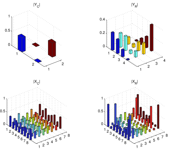
Figure 4: Magnitudes of primal-dual pairs $(X_{C},Y_{C})$ and $(X_{R},Y_{R})$ corresponding to $({\cal R}_{a100},{\mathcal{C}}_{a100})$ optimized for ${\mathcal{E}}_{a}$.

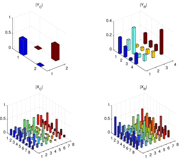
Figure 5: Magnitudes of primal-dual pairs $(X_{C},Y_{C})$ and $(X_{R},Y_{R})$ corresponding to $({\cal R}_{b100},{\mathcal{C}}_{b100})$ optimized for ${\mathcal{E}}_{b}$.

Appendix A Dual problem

We apply Lagrange Duality Theory [BV04, Ch.5]. Write the primal problem (23) as a minimization,

$$\begin{array}[]{ll}\mbox{minimize}&-{\bf Tr}\ XW\\ \mbox{subject to}&X\geq 0,\;\;\sum_{ij}X_{ij}C_{ij}=I_{m}\end{array}$$ (27)

with optimization variable $X=X^{\dagger}\in{\bf C}^{n\times n}$. The Lagrangian for (27) is,

$$\begin{array}[]{rcl}L(X,Z,Y)&=&-{\bf Tr}\ XW={\bf Tr}\ XZ-{\bf Tr}\ Y(I_{m}-\sum_{ij}X_{ij}B_{i}^{\dagger}B_{j})\\ &=&\sum_{ij}\ X_{ij}(-W_{ji}-Z_{ji}+{\bf Tr}\ YC_{ji})-{\bf Tr}\ Y\end{array}$$ (28)

where $Z=Z^{\dagger}\in{\bf C}^{n\times n}$ and $Y=Y^{\dagger}\in{\mathbf{C}}^{m\times m}$ are Lagrange multipliers associated with the (Hermitian) inequality and equality constraints, respectively. The Lagrange dual function is then,

$$\begin{array}[]{rcl}g(Z,Y)&=&\inf_{X}\ L(X,Z,Y)\\ &=&\left\{\begin{array}[]{ll}-{\bf Tr}\ Y&Z_{ji}={\bf Tr}\ YC_{ij}-W_{ji}\\ -\infty&\mbox{otherwise}\end{array}\right.\end{array}$$ (29)

For any $Y$ and $Z\geq 0$, $g(Z,Y)$ yields a lower bound on the optimal objective $-{\bf Tr}\ X^{\rm opt}W$. The largest lower bound from this dual function is then $\max\left\{\,g(Z,Y)\,\left|\,Z\geq 0\,\right.\right\}$. Eliminating $Z$, this can be written equivalently as,

$$\begin{array}[]{ll}\mbox{minimize}&{\bf Tr}\ Y\\ \mbox{subject to}&K(Y)-W\geq 0,\;\;K_{ij}(Y)={\bf Tr}\ YC_{ij}\end{array}$$ (30)

with optimization variable $Y=Y^{\dagger}\in{\mathbf{C}}^{m\times m}$. This is precisely the result in (24). Because the problem is strictly convex, the dual optimal objective is equal to the primal optimal objective as stated in the first line of (25). The complementary slackness condition gives the second line in (25).

References

• [ALZ05] R. Alicki, D.A. Lidar, and P. Zanardi. Internal Consistency of Fault-Tolerant Quantum Error Correction in Light of Rigorous Derivations of the Quantum Markovian Limit. Phys. Rev. A, 73, 052311, 2006.
• [BV04] S. Boyd and L. Vandenberghe. Convex Optimization. Cambridge University Press, 2004.
• [FSW06] A. S. Fletcher, P. W. Shor, and M. Z. Win. Optimum quantum error recovery using semidefinite programming. arXiv: quant-ph/0606035, 5 June 2006.
• [GL83] G. H. Golub and C. F. Van Loan. Matrix Computations. Johns Hopkins University Press, 1983.
• [G96] D. Gottesman. Class of quantum error-correcting codes saturating the quantum Hamming bound. Phys. Rev. A 54, 1862, 1996.
• [GLN05] A. Gilchrist, N. K. Langford, and M. A. Nielsen. Distance measures to compare real and ideal quantum processes. Phys. Rev. A, 71, (062310), 2005.
• [KWR04] R. L. Kosut, I. A. Walmsley and H. Rabitz. Optimal experiment design for quantum state and process tomography and Hamiltonian parameter estimation. arXiv:quant-ph/0411093, Nov 2004.
• [KGBR06] R. L. Kosut, M. Grace, C. Brif, and H. Rabitz. On the distance between unitary propagators of quantum systems of differing dimensions. arXiv: quant-ph/0606064, 8 June 2006.
• [KL97] E. Knill and R. Laflamme. Theory of quantum error-correcting codes. Phys. Rev. A, 55, 900, 1997.
• [LCW98] D.A. Lidar, I.L. Chuang, and K.B. Whaley. Decoherence-free subspaces for quantum computation. Phys. Rev. Lett., 81, 2594–2597, 1998.
• [NC00] M. A. Nielsen and I. L. Chuang. Quantum Computation and Quantum Information. Cambridge, 2000.
• [RW05] M. Reimpell and R. F. Werner. Iterative optimization of quantum error correcting codes. Phys. Rev. Lett., 94, 2005.
• [RWA06] M. Reimpell, R. F. Werner and K. Audenaert. Comment on “Optimum quantum error recovery using semidefinite programming.” arXiv: quant-ph/0606059, 7 June 2006.
• [S95] P. W. Shor. Scheme for reducing decoherence in quantum memory. Phys. Rev. A, 52, R2493, 1995.
• [S96] A. M. Steane. Error correcting codes in quantum theory. Phys. Rev. Lett. 77, 793, 1996.
• [YHT05] N. Yamamoto, S. Hara, and K. Tsumara. Suboptimal quantum error correcting procedure based on semidefinite programming. Phys. Rev. A, 71, 2005.
• [ZL04] P. Zanardi and D. Lidar. Purity and state fidelity of quantum channels. Phys. Rev. A, 70, 01235, 2004.