Conservative chaotic map as a model of quantum many-body environment

Abstract

We study the dynamics of the entanglement between two qubits coupled to a common chaotic environment, described by the quantum kicked rotator model. We show that the kicked rotator, which is a single-particle deterministic dynamical system, can reproduce the effects of a pure dephasing many-body bath. Indeed, in the semiclassical limit the interaction with the kicked rotator can be described as a random phase-kick, so that decoherence is induced in the two-qubit system. We also show that our model can efficiently simulate non-Markovian environments.

I Introduction

Real physical systems are never isolated and the coupling of the system to the environment leads to decoherence. This process can be understood as the loss of quantum information, initially present in the state of the system, when non-classical correlations (entanglement) establish between the system and the environment. On the other hand, when tracing over the environmental degrees of freedom, we expect that the entanglement between internal degrees of freedom of the system is reduced or even destroyed. Decoherence theory has a fundamental interest, since it provides explanations of the emergence of classicality in a world governed by the laws of quantum mechanics zurek . Moreover, it is a threat to the actual implementation of any quantum computation and communication protocol chuang ; qcbook . Indeed, decoherence invalidates the quantum superposition principle, which is at the heart of the potential power of any quantum algorithm. A deeper understanding of the decoherence phenomenon seems to be essential to develop quantum computation technologies.

The environment is usually described as a many-body quantum system. The best-known model is the Caldeira-Leggett model caldeiraleggett , in which the environment is a bosonic bath consisting of infinitely many harmonic oscillators at thermal equilibrium. More recently, first studies of the role played by chaotic dynamics in the decoherence process have been carried out park ; blume03 ; lee ; saraceno ; seligman . These investigations mainly focused on the differences between the processes of decoherence induced by chaotic and regular environments.

In this paper, we address the following question: could the many-body environment be substituted, without changing the effects on system’s dynamics, by a closed deterministic system with a small number of degrees of freedom yet chaotic? In other words, can the complexity of the environment arise not from being many-body but from chaotic dynamics? In this paper, we give a positive answer to this question. We consider two qubits coupled to a single particle, fully deterministic, conservative chaotic “environment”, described by the kicked rotator model. We show that, due to this system-environment interaction, the entropy of the system increases. At the same time, the entanglement between the two qubits decays, thus illustrating the loss of quantum coherence. We show that the evolution in time of the two-qubit entanglement is in good agreement with the evolution obtained in a pure dephasing stochastic model. Since this pure dephasing decoherence mechanism can be derived in the framework of the Caldeira-Leggett model palma , we have established a direct link between the effects of a many-body environment and of a chaotic single-particle environment.

Finally, we show that also non-Markovian effects naturally appear in our model. This is interesting since such effects are relevant in several implementations of quantum information protocols esteve , for instance with solid-state devices due to the coupling of the qubits to “slow” modes such as phonons. Moreover, non-Markovian effects, apart from some exceptions daffer , are usually very hard for analytic treatment. On the other hand, they can be included in models similar to the one discussed in the present paper with no additional computational cost with respect to the Markovian case.

The structure of the paper is as follows: in Sec. II our model of a chaotic environment is introduced; in Sec. III both the entropy production and the entanglement decay are investigated, and the results compared with those obtained in the phase-kick model; in Sec. IV non-Markovian effects are analyzed; our conclusions are drawn in Sec. V. The Bloch representation of the phase-kick map and the short time decay of the relevant bath (kicked rotator) correlation functions are discussed in Appendix A and Appendix B, respectively.

II The model

We consider two qubits coupled to a quantum kicked rotator. The overall system is governed by the Hamiltonian

$$\hat{H}=\hat{H}^{(1)}+\hat{H}^{(2)}+\hat{H}^{(\mathrm{kr})}+\hat{H}^{(\mathrm{int})}\,,$$ (1)

where $\hat{H}^{(i)}=\omega_{i}\,\hat{\sigma}_{x}^{(i)}$ ($i=1,2$) describes the free evolution of the two qubits,

$$\hat{H}^{(\mathrm{kr})}=\frac{\hat{n}^{2}}{2}+k\cos(\hat{\theta})\sum_{j}\delta(\tau-jT)$$ (2)

the quantum kicked rotator, and

$$\hat{H}^{(\mathrm{int})}=\epsilon\>(\hat{\sigma}_{z}^{(1)}+\hat{\sigma}_{z}^{(2)})\cos(\hat{\theta})\sum_{j}\delta(\tau-jT)$$ (3)

the interaction between the qubits and the kicked rotator; $\hat{\sigma}_{\alpha}^{(i)}$ ($\alpha=x,y,z$) denote the Pauli matrices of the $i$-th qubit. Both the cosine potential in $\hat{H}^{(\mathrm{kr})}$ and the interaction $\hat{H}^{(\mathrm{int})}$ are switched on and off instantaneously (kicks) at regular time intervals $T$. We consider the two qubits as an open quantum system and the kicked rotator as their common environment. Note that we chose noninteracting qubits as we want their entanglement to be affected exclusively by the coupling to the environment.

The evolution from time $tT$ (prior to the $t$-th kick) to time $(t+1)T$ (prior to the $(t+1)$-th kick) of the kicked rotator in the classical limit is described by the Chirikov standard map:

$$\left\{\begin{array}[]{l}\bar{n}=n+k\sin\theta,\\ \bar{\theta}=\theta+T\bar{n},\hskip 28.45274pt(\textrm{mod }2\pi),\end{array}\right.$$ (4)

where $(n,\theta)$ are conjugated momentum-angle variables. Hereafter $t=\tau/T$ denotes the discrete time, measured in number of kicks. By rescaling $n\to p=Tn$, the dynamics of Eqs. (4) is seen to depend only on the parameter $K=kT$. For $K=0$ the motion is integrable; when $K$ increases, a transition to chaos of the KAM type is observed. The last invariant KAM torus is broken for $K\approx 0.97$. If $K\sim 1$ the phase space is mixed (simultaneous presence of integrable and chaotic components). If $K$ increases further, the stability islands progressively reduce their size; for $K\gg 1$ they are not visible any more. In this paper, we always consider map (4) on the torus $0\leq\theta<2\pi$, $-\pi\leq p<\pi$. In this case, the Chirikov standard map describes the stroboscopic dynamics of a conservative dynamical system with two degrees of freedom which, in the fully chaotic regime $K\gg 1$, relaxes, apart from quantum fluctuations, to the uniform distribution on the torus.

The Hilbert space of the global system is given by

$$\mathcal{H}=\mathcal{H}^{(1)}\otimes\mathcal{H}^{(2)}\otimes\mathcal{H}^{(kr)}\,,$$ (5)

where $\mathcal{H}^{(1)}$ and $\mathcal{H}^{(2)}$ are the two-dimensional Hilbert spaces associated to the two qubits, and $\mathcal{H}^{(kr)}$ is the $N$-dimensional space for the kicked rotator.

The time evolution generated by Hamiltonian (1) in one kick is described by the operator

$$\begin{array}[]{rl}\hat{U}=&\exp\big{[}-i\big{(}k+\epsilon(\hat{\sigma}_{z}^{(1)}+\hat{\sigma}_{z}^{(2)})\big{)}\cos(\hat{\theta})\big{]}\\ &\times\,\exp\big{[}-iT\frac{\hat{n}^{2}}{2}\big{]}\exp\big{(}-i\,\delta_{1}\,\hat{\sigma}_{x}^{(1)}\big{)}\exp\big{(}-i\,\delta_{2}\,\hat{\sigma}_{x}^{(2)}\big{)}.\end{array}$$ (6)

The effective Planck constant is $\hbar_{\textrm{eff}}=T=2\pi/N$, where $N$ is the number of quantum levels used to describe the kicked rotator; $\delta_{1}=\omega_{1}T,\>\delta_{2}=\omega_{2}T$; $\epsilon$ is the coupling strength between the qubits and the environment. The classical limit $\hbar_{\textrm{eff}}\to 0$ is obtained by taking $T\to 0$ and $k\to\infty$, in such a way that $K=kT$ is kept fixed.

III Loss of coherence induced by a chaotic environment

We are interested in the case in which the environment (the kicked rotator) is chaotic (we consider the kicked rotator with $K\gg 1$). The two qubits are initially prepared in a maximally entangled state, such that they are disentangled from the environment. Namely, we suppose that at $t=0$ the system is in the state

$$\left|\Psi_{0}\right\rangle=\left|\phi^{+}\right\rangle\otimes\left|\psi_{0}\right\rangle\,,$$ (7)

where $\left|\phi^{+}\right\rangle=\frac{1}{\sqrt{2}}\left(\left|00\right\rangle+\left|11\right\rangle\right)$ is a Bell state (the particular choice of the initial maximally entangled state is not crucial for our purposes), and $\left|\psi_{0}\right\rangle=\sum_{n}c_{n}\left|n\right\rangle$ is a generic state of the kicked rotator, with $c_{n}$ random coefficients such that $\sum_{n}\left|c_{n}\right|^{2}=1$, and $\left|n\right\rangle$ eigenstates of the momentum operator. The evolution in time of the global system (kicked rotator plus qubits) is described by the unitary operator $\hat{U}$ defined in Eq. (6). Therefore, any initial pure state $\left|\Psi_{0}\right\rangle$ evolves into another pure state $\left|\Psi(t)\right\rangle=\hat{U}^{t}\left|\Psi_{0}\right\rangle$. The reduced density matrix $\rho_{12}(t)$ describing the two qubits at time $t$ is then obtained after tracing $\left|\Psi(t)\right\rangle\left\langle\Psi(t)\right|$ over the kicked rotator’s degrees of freedom.

In the following we will focus our attention on the time evolution of the entanglement $E_{12}$ between the two qubits and between them and the kicked rotator, measured by the reduced von Neumann entropy $S_{12}$. Clearly, for states like the one in Eq. (7), we have $E_{12}(0)=1$, $S_{12}(0)=0$. As the total system evolves, we expect that $E_{12}$ decreases, while $S_{12}$ grows up, thus meaning that the two-qubit system is progressively losing coherence.

The entanglement of formation $E_{12}$ of a generic two-qubit state $\rho_{12}$ can be evaluated following Ref. wootters98 . First of all we compute the concurrence, defined as $C=\max(\lambda_{1}-\lambda_{2}-\lambda_{3}-\lambda_{4},0)$, where the $\lambda_{i}$’s are the square roots of the eigenvalues of the matrix $R=\rho_{12}\tilde{\rho}_{12}$, in decreasing order. Here $\tilde{\rho}_{12}$ is the spin flipped matrix of $\rho_{12}$, and it is defined by $\tilde{\rho}_{12}=(\sigma_{y}\otimes\sigma_{y})\,\rho_{12}^{\star}\,(\sigma_{y}\otimes\sigma_{y})$ (note that the complex conjugate is taken in the computational basis $\{|00\rangle,|01\rangle,|10\rangle,|11\rangle\}$). Once the concurrence has been computed, the entanglement of formation is obtained as $E=h((1+\sqrt{1-C^{2}})/2)$, where $h$ is the binary entropy function: $h(x)=-x\log_{2}x-(1-x)\log_{2}(1-x)$, with $x=(1+\sqrt{1-C^{2}})/2$. The other quantity studied in our investigations is the entanglement between the two qubits and the kicked rotator, measured by the von Neumann entropy $S=-\mathrm{Tr}\,[\rho_{12}\log_{2}\rho_{12}]$ of the reduced density matrix $\rho_{12}$.

If the kicked rotator is in the chaotic regime and in the semiclassical region $\hbar_{\textrm{eff}}\ll 1$, it is possible to drastically simplify the description of the system in Eq. (1) by using the random phase-kick approximation, in the framework of the Kraus representation formalism. Since, to a first approximation, the phases between two consecutive kicks in the chaotic regime can be considered as uncorrelated, the interaction with the environment can be simply modeled as a phase-kick rotating both qubits through the same random angle about the $z$-axis of the Bloch sphere. This rotation is described by the unitary matrix

$$\hat{R}(\theta)=\left[\begin{array}[]{cc}e^{-i\epsilon\cos\theta}&0\\ 0&e^{i\epsilon\cos\theta}\end{array}\right]\otimes\left[\begin{array}[]{cc}e^{-i\epsilon\cos\theta}&0\\ 0&e^{i\epsilon\cos\theta}\end{array}\right],$$ (8)

where the angle $\theta$ is drawn from a uniform random distribution in $[0,2\pi)$. The one-kick evolution of the reduced density matrix $\rho_{12}$ is then obtained after averaging over $\theta$:

$$\begin{array}[]{c}\bar{\rho}_{12}=\frac{1}{2\pi}\int_{0}^{2\pi}d\theta\,\hat{R}(\theta)\,e^{-i\delta_{2}\hat{\sigma}_{x}^{(2)}}e^{-i\delta_{1}\hat{\sigma}_{x}^{(1)}}\vspace{1mm}\\ \times\,\rho_{12}\,e^{i\delta_{1}\hat{\sigma}_{x}^{(1)}}e^{i\delta_{2}\hat{\sigma}_{x}^{(2)}}\hat{R}^{\dagger}(\theta).\end{array}$$ (9)

In order to assess the validity of the random phase-kick approximation, we numerically investigate model (1) in the classically chaotic regime $K\gg 1$ and in the region $\hbar_{\textrm{eff}}\ll 1$ in which the environment is a semiclassical object. Under these conditions, we expect that the time evolution of the entanglement can be accurately predicted by the random phase model. Such expectation is confirmed by the numerical data shown in Fig. 1. Even though differences between the two models remain at long times due to the finite number $N$ of levels in the kicked rotator, such differences appear at later and later times when $N\to\infty$ ($\hbar_{\textrm{eff}}\to 0$). The parameter $K$ has been chosen much greater than one, so that the classical phase space of the kicked rotator can be considered as completely chaotic. The actual value $K\approx 99.72676$ approximately corresponds to a zero of the Bessel function $J_{2}(K)$. This is to completely wipe off memory effects between consecutive and next-consecutive kicks (see Sec. IV, Eqs. (13)-(14) for details).

Figure 1: Reduced von Neumann entropy $S_{12}$ (main figure) and entanglement $E_{12}$ (inset) as a function of time at $K\approx 99.73$, $\delta_{1}=10^{-2}$, $\delta_{2}=\sqrt{2}\delta_{1}$, $\epsilon=8\times 10^{-3}$. The thin curves correspond to different number of levels for the environment (the kicked rotator) ($N=2^{9},2^{10},2^{11},2^{12},2^{13},2^{14}$ from bottom to top in the main figure and vice versa in the inset). The thick curves give the numerical results from the random phase model (9).

We point out that the random phase model can be derived from the Caldeira-Leggett model with a pure dephasing coupling $\propto(\hat{\sigma}_{z}^{(1)}+\hat{\sigma}_{z}^{(2)})\sum_{k}g_{k}\hat{q}_{k}$, with $g_{k}$ coupling constant to the $k$-th oscillator of the environment, whose coordinate operator is $\hat{q}_{k}$ palma ; braun . This establishes a direct link between our chaotic single-particle environment and a standard many-body environment.

Numerical simulations show that, when the kicked rotator is chaotic, the pairwise entanglement $E_{12}$ between the two qubits decays exponentially at short times, with a rate $\Gamma$ proportional to $\epsilon^{2}$:

$$E_{12}(t)\sim e^{-\alpha\epsilon^{2}t}\,.$$ (10)

This is clearly seen from Figs. 2 and 3 lewenstein . In Fig. 2 we plot the decay of entanglement $E_{12}$ in time, for different values of the oscillation frequencies $\delta_{1}$ and $\delta_{2}$ of the two qubits, at a fixed value of the coupling strength $\epsilon$ with the environment. The short time decay of $E_{12}$ is always exponential and superimposed to oscillations whose frequency is determined by the internal dynamics of the two qubits note_frequencies . Such oscillations can be clearly seen for $\delta_{1}=\delta_{2}/\sqrt{2}=10^{-3}$ (dashed curve), while their amplitude and period are too small to be seen on the scale of the figure for $\delta_{1}=\delta_{2}/\sqrt{2}=10^{-1}$ (solid curve). Finally, oscillations are absent at $\delta_{1}=\delta_{2}/\sqrt{2}=10^{-4}$ (dotted curve), as in this case their period is longer than the time scale for entanglement decay. Analogous remarks can be done about the oscillations in the entanglement production, measured by the reduced von Neumann entropy plotted in the inset of Fig. 2.

Figure 2: Entanglement $E_{12}$ as a function of time for two qubits coupled to a chaotic kicked rotator ($K\approx 99.73$) with $N=2^{14}$ levels and coupling strength $\epsilon=0.016$. The various curves are for different oscillation frequencies of the qubits: $\delta_{1}=\delta_{2}/\sqrt{2}=10^{-1},\textrm{(solid curve)},\>10^{-3}\,\textrm{(dashed curve)},\>10^{-4}\textrm{(dotted curve)}$. The thick dashed line gives the analytic estimate (11), valid in the regime $\delta_{1},\delta_{2}\ll\epsilon\ll 1$. Inset: same as in the main figure but for the Von Neumann entropy $S_{12}$. The thick dashed curve is the estimate (12).

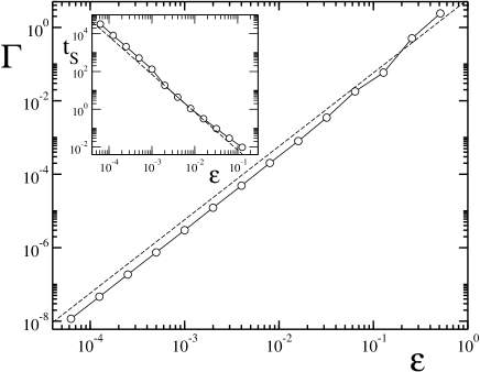
Figure 3: Decay rates $\Gamma$ of the entanglement $E_{12}$ (main figure) and time scales $t_{S}$ for the Von Neumann entropy (obtained from $S_{12}(t_{S})=0.002$) (inset) as a function of the coupling strength $\epsilon$ for $N=2^{14}$, $K\approx 99.73$, $\delta_{1}=\delta_{2}/\sqrt{2}=10^{-2}$. Both numerical data (circles) and the analytic predictions (dashed curves) given by Eq. (11) (main figure) and Eq. (12) (inset) are shown.

An analytic estimate of the entanglement decay rate and of the entropy production can be derived from the random phase-kick model, in the limiting case $\delta_{1},\delta_{2}\ll\epsilon\ll 1$, that is, when the internal dynamics of the two qubits can be neglected on the time scale for entanglement decay. Starting from Eq. (9), it is possible to explicitly write down the map $\rho_{12}\to\bar{\rho}_{12}$ in the Bloch representation, see Eqs. (23) in App. A. Though in general these equations have to be solved numerically, in App. A we provide an explicit analytic solution valid for $\delta_{1},\delta_{2}\ll\epsilon\ll 1$. In that case, for $\epsilon^{2}t\ll 1$ we obtain:

$$E_{12}(t) \simeq 1-\frac{4\epsilon^{2}t}{\ln 2},$$ (11)

$$S_{12}(t) \simeq \frac{2\epsilon^{2}t}{\ln 2}\left(1-\ln(2\epsilon^{2}t)\right),$$ (12)

consistently with the numerically obtained behavior of Eq. (10) for small times, with $\alpha\approx 4/\ln 2$. The analytic estimates (11) for $E_{12}$ and (12) for $S_{12}$ are shown as thick dashed curves in Fig. 2. A very good agreement with numerical data can be clearly seen for $\delta_{1},\delta_{2}\ll\epsilon\ll 1$.

In Fig. 3 the decay rate $\Gamma$ of entanglement as a function of $\epsilon$ is shown; circles represent numerical data, while the dashed line is the analytic estimate of Eq. (11). A dependence $\Gamma\propto\epsilon^{2}$ is found in both cases. In the inset we plot the characteristic time scale $t_{S}$ for the von Neumann entropy production. The time scale $t_{S}$ has been determined from the condition $S_{12}(t_{S})=C=0.002$ (the value chosen for $C$ is not crucial). As before, circles stand for numerical data, while the dashed line is obtained from Eq. (12). From this figure we can conclude that the dependences of both $\Gamma$ and $t_{S}$ on the system-environment coupling strength $\epsilon$ are correctly reproduced by Eqs. (11) and (12), even though the oscillations due to the internal system’s dynamics cannot be reproduced by these analytic estimates. Finally, we point out that, as clear from Fig. 1, in the semiclassical chaotic regime ($\hbar_{\textrm{eff}}\ll 1$ and $K\gg 1$) both $\Gamma$ and $t_{S}$ can be reproduced with great accuracy by the random phase-kick model.

We would like to stress that the results discussed in this section do not depend on the initial condition $|\psi_{0}\rangle$ in (7), provided that the kicked rotator is in the chaotic regime. On the other hand, we have found that both the entanglement decay and the entropy production strongly depend on $|\psi_{0}\rangle$ in the integrable region $K<1$. This implies that only in the chaotic regime a single particle can behave as a dephasing environment.

Finally we notice that, contrary to other bath models braun , the random phase-kick model does not generate entanglement between the two qubits. This has been numerically checked for model (1) both for initial pure separable states and for separable mixtures. Moreover we also checked that, starting from a generic two qubit entangled state, the interaction with a chaotic memoryless environment cannot increase entanglement. Namely, we considered $10^{7}$ random initial conditions with $E_{12}(0)\neq 0$ and we found that, already after $t\sim 100$ kicks, entanglement has been always lowered: $E_{12}(t)<E_{12}(0)$.

IV Non-Markovian effects

The model governed by Eq. (1) is very convenient for numerical investigations of decoherence. It can also be used to study physical situations which cannot be easily treated by means of analytic techniques using many-body environments like in the Caldeira-Leggett model. For instance, one could simulate, with the same computational cost, more complex couplings (e.g. when the direction of the coupling changes in time) or non-Markovian environments.

In this section, we show that memory effects naturally appear in our model, outside the range of validity of the random phase approximation. First of all, we point out that, given the coupling $\hat{H}^{(\mathrm{int})}\propto\cos\hat{\theta}$, the bath correlation function relevant for the study of memory effects is $\langle\cos[\theta(t)]\cos[\theta(t^{\prime})]\rangle$. Even in the chaotic regime, the phases are not completely uncorrelated: in the classical Chirikov standard map (4) correlations between cosines of the phases in two consecutive kicks are zero, but the same correlations between phases of two next-consecutive kicks do not vanish. As shown in Appendix B, we have

$$\langle\cos\theta\cos\bar{\theta}\rangle = 0,$$ (13)

$$\langle\cos\theta\cos\bar{\bar{\theta}}\rangle = \frac{J_{2}(K)}{2},$$ (14)

where, given $\theta=\theta(t)$, $\bar{\theta}=\theta(t+1)$ and $\bar{\bar{\theta}}=\theta(t+2)$, $J_{2}(K)$ is the Bessel function of the first kind of index 2 and $K$ is the classical chaos parameter. Correlations between more distant kicks, $\langle\cos[\theta(t)]\cos[\theta(t^{\prime})]\rangle$, with $t^{\prime}-t>2$, though non vanishing, are very weak for $K\gg 1$, therefore hereafter we will neglect them. Correlations in the kicked rotator dynamics eventually result in a modification of the decay rate $\Gamma$ of entanglement, as it is clearly shown in Fig. 4, where we plot the dependence of $\Gamma$ as a function of $K$.

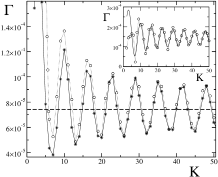
Figure 4: Oscillations of the entanglement decay rate $\Gamma$ as a function of the classical chaos parameter $K$, at $\epsilon=5\times 10^{-3},\delta_{1}=\delta_{2}/\sqrt{2}=10^{-2}$, $N=2^{14}$ (circles). Stars show the results obtained from a quantum trajectory approach (with average over 5000 trajectories) applied to the phase-kick model (16). Inset: entanglement decay rates as a function of $K$ for $\epsilon=5\times 10^{-3}$, $\delta_{1}=\delta_{2}=0$, $N=2^{14}$ (circles). The solid curve shows the analytic estimate (18).

In order to study analytically memory effects on the entanglement decay, we provide a simple generalization of the random phase-kick model (9), so that the correlations of Eqs. (13)-(14) are taken into account. We use the following conditional probability distribution for the angle $\bar{\theta}$ at time $t+1$, given the angle $\theta$ at time $t$:

$$p(\bar{\theta}|\theta)=\left\{\begin{array}[]{ll}\displaystyle\sqrt{J_{2}}\>\delta\left[\bar{\theta}-\theta+\frac{\pi}{2}(-1)^{t}\right]+\frac{1-\sqrt{J_{2}}}{2\pi},&(J_{2}>0),\vspace{1mm}\\ \displaystyle\sqrt{-J_{2}}\>\delta\left[\bar{\theta}-\theta-\frac{\pi}{2}\right]+\frac{1-\sqrt{-J_{2}}}{2\pi},&(J_{2}<0).\end{array}\right.$$ (15)

This distribution corresponds to having a $\bar{\theta}$ angle which is correlated with $\theta$ (i.e. $\bar{\theta}=\theta\pm\pi/2$) with probability $p_{\mathrm{c}}=\sqrt{\left|J_{2}\right|}$, and completely uncorrelated with probability $p_{\mathrm{nc}}=1-p_{\mathrm{c}}$. For our purposes, the relevant properties of the probability distribution $p(\theta,\bar{\theta})=p(\theta)p(\bar{\theta}|\theta)$ are: $\int d\theta\int d\bar{\theta}\,p(\theta,\bar{\theta})=1$; $\int d\theta\int d\bar{\theta}\,p(\theta,\bar{\theta})\cos\theta\cos\bar{\theta}=0$; $\int d\theta\int d\bar{\theta}\,p(\theta,\bar{\bar{\theta}})\cos\theta\cos\bar{\bar{\theta}}=J_{2}/2$. Therefore, Eq. (15) is a convenient distribution probability leading to a decay of the bath correlation function as in Eqs. (13)-(14) for the kicked rotator model. Of course, other probability distributions could equally well reproduce such decay.

Given the probability distribution $p(\bar{\theta}|\theta)$, we can replace (9) with the following two-kicks time evolution map:

$$\begin{array}[]{l}\bar{\bar{\rho}}_{12}=\displaystyle\int_{0}^{2\pi}d\theta\,\int_{0}^{2\pi}d\bar{\theta}\,p(\theta,\bar{\theta})\,\hat{R}(\bar{\theta})\hat{R}({\theta})\,\rho_{12}\,\hat{R}^{\dagger}({\theta})\hat{R}^{\dagger}(\bar{\theta}),\end{array}$$ (16)

where $\rho_{12}$ and $\bar{\bar{\rho}}_{12}$ denote the two-qubit density matrix at times $t$ and $t+2$ and $p(\theta,\bar{\theta})$ is the joint probability to have a rotation through an angle $\theta$ at a time $t$ and through an angle $\bar{\theta}$ at time $t+1$. Therefore, $p(\theta,\bar{\theta})$ accounts for correlations between the angles at subsequent kicks. Clearly, if angles are completely uncorrelated we have $p(\theta,\bar{\theta})=1/4\pi^{2}$, thus recovering the random phase-kick model (9). Note that, for the sake of simplicity, map (16) has been written for $\delta_{1}=\delta_{2}=0$ (the generalization of this map to $\delta_{1},\delta_{2}\neq 0$ is straightforward).

The phase-kick model (16) can be simulated by using the quantum trajectories approach carmichael ; brun ; carlo . This method is very convenient in the study of dissipative systems: instead of solving a master equation, one stochastically evolves a state vector, and then averages over many runs. At the end, we get the same probabilities as the ones directly obtained through the density matrix. In our case, the effect of the kicked rotator on the two-qubits wave function is simply that of a rotation through an angle whose value is drawn according to the probability distribution (15). Numerical data obtained with the quantum trajectories method are plotted in Fig. 4 (stars); notice that, at $K\gg 1$, they are in good agreement with data from simulation of the Hamiltonian model (1) (circles).

It is also possible to give an analytic estimate of the decay rate $\Gamma(K)$ in the limit in which the free evolution of the two qubits can be neglected (i.e., we take $\delta_{1},\delta_{2}\ll\epsilon\ll 1$). As for the random phase model (9), in this limit the effect of map (16) is pure dephasing. At every map step the density matrix $\rho_{12}$ is of the form of Eq. (26). The coherences $D_{t}$ can be computed by iterating Eq. (16). We obtain what follows for the first time steps:

$$\left\{\begin{array}[]{l}D_{1}=1-4\epsilon^{2},\vspace{0.3mm}\\ D_{2}=1-8\epsilon^{2},\vspace{0.3mm}\\ D_{3}=1-\big{[}12+8J_{2}(K)\big{]}\epsilon^{2},\vspace{0.3mm}\\ D_{4}=1-\big{[}16+16J_{2}(K)\big{]}\epsilon^{2}.\vspace{0.3mm}\end{array}\right.$$ (17)

Assuming an exponential decay of entanglement, $E_{12}(t)\sim e^{-\Gamma t}$, we can evaluate $\Gamma$ starting from $D_{3}$ and $D_{4}$: $\Gamma\approx\ln(E_{3}/E_{4})$. Thus, from Eqs. (17) we obtain the following analytic estimate:

$$\Gamma\approx\frac{4\epsilon^{2}}{\ln 2}\left(1+2J_{2}(K)\right).$$ (18)

In the inset of Fig. 4 we compute the entanglement decay rates as a function of $K$ in the case $\delta_{1}=\delta_{2}=0$. This figure clearly shows that the rates obtained from numerical data for the chaotic environment model (circles) are in good agreement, when $K\gg 1$, with the analytic estimate (18) (solid curve).

We point out that the oscillations with $K$ of the entanglement decay rate $\Gamma(K)$ are ruled by the Bessel function $J_{2}(K)$, in the same way as for the well-known $K$-oscillations of the classical diffusion coefficient $D(K)$ rechester80 . Therefore, the entanglement decay rate is strictly related to a purely classical quantity. The ultimate reason of this relation is rooted in the fact that the bath correlation function relevant for the study of memory effects, $\langle\cos[\theta(t)]\cos[\theta(t^{\prime})]\rangle$, also determines the deviations of the diffusion coefficient $D(K)$ from the random phase approximation value $K^{2}/2$.

V Conclusions

We have shown that a single particle in the chaotic regime can be equivalent to a bath with infinitely many degrees of freedom as a dephasing environment. This provides a clear example of the relevance of chaos to decoherence. Furthermore, also memory effects can be included in a single particle chaotic environment. This observation paves the way to a convenient numerical simulation of non-Markovian dynamics. Indeed, both exponential and power-law decays of the bath (single particle) correlation functions can be obtained in chaotic maps sawtooth ; liverani . Therefore, these maps could be used to efficiently simulate important quantum noise models such as random telegraphic or $1/f$ noise.

Appendix A The random phase model

Here we provide an explicit set of equations describing map (9) in the Bloch representation. In such representation, a generic two-qubit mixed state can be written as

$$\rho_{12}=\frac{1}{4}\hat{\mathbb{I}}\otimes\hat{\mathbb{I}}+\sum_{i=1}^{3}\alpha_{i}(\hat{\sigma}_{i}\otimes\hat{\mathbb{I}})+\sum_{j=1}^{3}\beta_{j}(\hat{\mathbb{I}}\otimes\hat{\sigma}_{j})+\sum_{i,j=1}^{3}\gamma_{ij}(\hat{\sigma}_{i}\otimes\hat{\sigma}_{j})$$ (19)

We insert this expansion into Eq. (9) and evaluate the commutators between $\rho_{12}$ and the terms that multiply $\rho_{12}$ on the right in (9) ($e^{i\delta_{1}\hat{\sigma}_{x}^{(1)}}$, $e^{i\delta_{2}\hat{\sigma}_{x}^{(2)}}$, and $\hat{R}^{\dagger}(\theta)$). For this purpose, we use the standard commutation rules for the Pauli matrices:

$$\left[\hat{\sigma}_{i},\hat{\sigma}_{j}\right]=2i\,\epsilon_{ijk}\,\hat{\sigma}_{k}\,,$$ (20)

where $\epsilon_{ijk}$ is the Levi-Civita tensor, which is equal to $+1$ if $ijk$ is an even permutation of $123$, to $-1$ for odd permutations and $0$ otherwise. We also use the identity

$$e^{i\delta\hat{\sigma}_{x}}=(\cos\delta)\,\hat{\mathbb{I}}+i\,(\sin\delta)\,\hat{\sigma}_{x}$$ (21)

and expand the exponentials in $\hat{R}^{\dagger}(\theta)$ to the second order in $\epsilon$. The average over $\theta$ is then performed using

$$\begin{array}[]{c}\left<\cos^{2n+1}\theta\right>_{\theta}=0,\vspace{2mm}\\ \qquad\left<\cos^{2}\theta\right>_{\theta}=\frac{1}{2},\qquad\left<\cos^{4}\theta\right>_{\theta}=\frac{3}{8}.\end{array}$$ (22)

In this way we arrive at the following one-kick map, valid in the approximation $\epsilon,\delta_{1},\delta_{2}\ll 1$:

$$\begin{array}[]{c}\left\{\begin{array}[]{l}\bar{\alpha}_{x}=\alpha_{x}(1-\epsilon^{2}),\\ \bar{\alpha}_{y}=\alpha_{y}(1-\epsilon^{2})-2\delta_{1}\alpha_{z},\\ \bar{\alpha}_{z}=\alpha_{z}+2\delta_{1}\alpha_{y},\end{array}\right.\vspace{2mm}\par\\ \left\{\begin{array}[]{l}\bar{\beta}_{x}=\beta_{x}(1-\epsilon^{2}),\\ \bar{\beta}_{y}=\beta_{y}(1-\epsilon^{2})-2\delta_{2}\beta_{z},\\ \bar{\beta}_{z}=\beta_{z}+2\delta_{2}\beta_{y},\end{array}\right.\vspace{2mm}\par\\ \left\{\begin{array}[]{l}\bar{\gamma}_{xx}=\gamma_{xx}(1-2\epsilon^{2})+2\epsilon^{2}\gamma_{yy},\\ \bar{\gamma}_{yy}=\gamma_{yy}(1-2\epsilon^{2})+2\epsilon^{2}\gamma_{xx}-2\delta_{1}\gamma_{zy}-2\delta_{2}\gamma_{yz},\\ \bar{\gamma}_{zz}=\gamma_{zz}+2\delta_{1}\gamma_{yz}+2\delta_{2}\gamma_{zy},\\ \bar{\gamma}_{xy}=\gamma_{xy}(1-2\epsilon^{2})-2\epsilon^{2}\gamma_{yx}-2\delta_{2}\gamma_{xz},\\ \bar{\gamma}_{yx}=\gamma_{yx}(1-2\epsilon^{2})-2\epsilon^{2}\gamma_{xy}-2\delta_{2}\gamma_{zx},\\ \bar{\gamma}_{xz}=\gamma_{xz}(1-2\epsilon^{2})+2\delta_{2}\gamma_{xy},\\ \bar{\gamma}_{zx}=\gamma_{zx}(1-2\epsilon^{2})+2\delta_{1}\gamma_{yx},\\ \bar{\gamma}_{yz}=\gamma_{yz}(1-2\epsilon^{2})-2\delta_{1}\gamma_{zz}+2\delta_{2}\gamma_{yy},\\ \bar{\gamma}_{zy}=\gamma_{zy}(1-2\epsilon^{2})+2\delta_{1}\gamma_{yy}-2\delta_{2}\gamma_{zz}.\end{array}\right.\par\end{array}$$ (23)

Note that these equations can be straightforwardly generalized to the continuous time limit.

We now focus on the case in which the two qubits are initially in the Bell state $\left|\phi^{+}\right\rangle$, so that the only non zero coordinates in the Bloch representation of $\rho_{12}(t=0)=\left|\phi^{+}\right\rangle\left\langle\phi^{+}\right|$ are $\gamma_{xx}=\gamma_{zz}=-\gamma_{yy}=1/4$. The system in Eq. (23) then reduces to a set of five coupled equations for the $\gamma$’s:

$$\left\{\begin{array}[]{l}\bar{\gamma}_{xx}=\gamma_{xx}(1-2\epsilon^{2})+2\epsilon^{2}\gamma_{yy},\\ \bar{\gamma}_{yy}=\gamma_{yy}(1-2\epsilon^{2})+2\epsilon^{2}\gamma_{xx}-2\delta_{1}\gamma_{zy}-2\delta_{2}\gamma_{yz},\\ \bar{\gamma}_{zz}=\gamma_{zz}+2\delta_{1}\gamma_{yz}+2\delta_{2}\gamma_{zy},\\ \bar{\gamma}_{yz}=\gamma_{yz}(1-2\epsilon^{2})-2\delta_{1}\gamma_{zz}+2\delta_{2}\gamma_{yy},\\ \bar{\gamma}_{zy}=\gamma_{zy}(1-2\epsilon^{2})+2\delta_{1}\gamma_{yy}-2\delta_{2}\gamma_{zz}.\end{array}\right.$$ (24)

Their solution after $t$ map steps is given, in the limiting case $\delta_{1},\delta_{2}\ll\epsilon\ll 1$, by

$$\gamma_{xx}(t)\approx-\gamma_{yy}(t)\approx\frac{1}{4}-\epsilon^{2}t,\quad\gamma_{zz}(t)\approx\frac{1}{4}.$$ (25)

Note that here we also require $\epsilon^{2}t\ll 1$. The corresponding density matrix is

$$\rho_{12}(t)=\frac{1}{2}\left(\begin{array}[]{cccc}1&0&0&D_{t}\\ 0&0&0&0\\ 0&0&0&0\\ D_{t}&0&0&1\end{array}\right),$$ (26)

with

$$D_{t}=1-4\epsilon^{2}t.$$ (27)

The calculation of the von Neumann entropy $S_{12}(t)$ and of the entanglement $E_{12}(t)$ for state (26) is straightforward and leads to Eqs. (11)-(12).

Appendix B Angular correlations in the Chirikov standard map

After rescaling the angular momentum $n\to p=Tn$, the Chirikov standard map (4) becomes

$$\left\{\begin{array}[]{l}\bar{p}=p+K\sin\theta,\\ \bar{\theta}=\theta+\bar{p},\hskip 28.45274pt(\textrm{mod }2\pi),\end{array}\right.$$ (28)

where $K=kT$. In this appendix we provide a simple proof of Eqs. (13)-(14), namely we evaluate correlations between the cosines of the phases of two consecutive and next-consecutive kicks. Averages are performed over all the input phase space:

$$\left<f(\theta,p)\right>\equiv\lim_{P\to\infty}\left\{\int_{-P}^{P}\frac{\rm{d}p}{2P}\>\int_{0}^{2\pi}\frac{f(\theta,p)}{2\pi}\,\rm{d}\theta\right\}$$ (29)

By using Eq. (28), we obtain the following equalities for correlations between two consecutive kicks:

$$\begin{array}[]{l}\displaystyle\left<\cos\theta\cos\bar{\theta}\right>=\left<\cos\theta\cos\left(\theta+p+K\sin\theta\right)\right>\vspace{1mm}\\ \displaystyle\hskip 14.22636pt=\left<\cos p\right>\left<\cos\theta\cos\left(\theta+K\sin\theta\right)\right>\vspace{1mm}\\ \displaystyle\hskip 14.22636pt-\,\left<\sin p\right>\left<\cos\theta\sin\left(\theta+K\sin\theta\right)\right>=0,\end{array}$$ (30)

where we have used some trivial trigonometric identities, and $\left<\cos x\right>=\left<\sin x\right>=0$.

Correlations between two next-consecutive kicks are evaluated by considering values at times $t+1$ (denoted by an overbar) and $t-1$ (denoted by an underbar). The map in Eq. (28) can be straightforwardly inverted to give backward evolution:

$$\left\{\begin{array}[]{l}\underline{p}=p-K\sin(\theta-p),\\ \underline{\theta}=\theta-p,\hskip 28.45274pt(\textrm{mod }2\pi).\end{array}\right.$$ (31)

Therefore, from Eqs. (28) and (31), after some simple algebra we obtain:

$$\begin{array}[]{l}\displaystyle\left<\cos\bar{\theta}\cos\underline{\theta}\right>=\left<\cos\left(\theta+p+K\sin\theta\right)\cos\left(\theta-p\right)\right>\\ \displaystyle=\frac{1}{2}\left<\cos\left(2\theta+K\sin\theta\right)\right>=\frac{1}{2}J_{-2}(K)=\frac{1}{2}J_{2}(K),\end{array}$$ (32)

where

$$J_{n}(K)=\frac{1}{2\pi}\int_{0}^{2\pi}\cos\left(K\sin\theta-n\theta\right)\textrm{d}\theta$$ (33)

is the Bessel function of the first kind of index 2.

References

- (1) W.H. Zurek, Rev. Mod. Phys. 75, 715 (2003).
- (2) M.A. Nielsen and I.L. Chuang, Quantum Computation and Quantum Information (Cambridge University Press, Cambridge, 2000).
- (3) G. Benenti, G. Casati, and G. Strini, Principles of Quantum Computation and Information, Vol. I: Basic concepts (World Scientific, Singapore, 2004).
- (4) A.O. Caldeira and A.J. Leggett, Ann. Phys. 149, 374 (1983).
- (5) H.-K. Park and S. W. Kim, Phys. Rev. A 67, 060102(R) (2003).
- (6) R. Blume-Kohout and W.H. Zurek, Phys. Rev. A 68, 032104 (2003).
- (7) J.W. Lee, D.V. Averin, G. Benenti, and D.L. Shepelyansky, Phys. Rev. A 72, 012310 (2005).
- (8) L. Ermann, J.P. Paz, and M. Saraceno, Phys. Rev. A 73, 012302 (2006).
- (9) C. Pineda and T.H. Seligman, quant-ph/0605169.
- (10) G.M. Palma, K.-A. Suominen, and A.K. Ekert, Proc. R. Soc. Lond. A 452, 567 (1996).
- (11) G. Ithier, E. Collin, P. Joyez, P.J. Meeson, D. Vion, D. Esteve, F. Chiarello, A. Shnirman, Y. Makhlin, J. Schriefl, and G. Schön, Phys. Rev. B 72, 134519 (2005).
- (12) S. Daffer, K. Wódkiewicz, J.D. Cresser, and J.K. McIver, Phys. Rev. A 70, 010304(R) (2004).
- (13) W.K. Wootters, Phys. Rev. Lett. 80, 2245 (1998).
- (14) D. Braun, Phys. Rev. Lett. 89, 277901 (2002).
- (15) Note that the entanglement decay cannot be exponential at long times. Indeed we have after a finite time (see Fig. 1), since the set of separable two-qubit mixed states possesses a nonzero volume [see K. Życzkowski, P. Horodecki, A. Sanpera, and M. Lewenstein, Phys. Rev. A 58, 883 (1998)], and enters this volume in a finite time.
- (16) In the limit in which one of the two qubits’ oscillation frequencies is much smaller than the other, the period of entanglement oscillations is given by . When the two frequencies are comparable (), then , where . In general is a non linear function of and ; this feature is contained in Eqs. (23), which have to be solved numerically for each specific case.
- (17) H.J. Carmichael, An Open Systems Approach to Quantum Optics (Springer, Berlin, 1993).
- (18) T.A. Brun, Am. J. Phys. 70, 719 (2002).
- (19) G.G. Carlo, G. Benenti and G. Casati, Phys. Rev. Lett. 91, 257903 (2003); G.G. Carlo, G. Benenti, G. Casati and C. Mejía-Monasterio, Phys. Rev. A 69, 062317 (2004).
- (20) A.B. Rechester, and R.B. White, Phys. Rev. Lett. 44, 1586 (1980); A.B. Rechester, M.N. Rosenbluth, and R.B. White, Phys. Rev. A 23, 2664 (1981).
- (21) G. Benenti, G. Casati, S. Montangero, and D.L. Shepelyansky, Phys. Rev. Lett. 87, 227901 (2001).
- (22) C. Liverani and M. Martens, Commun. Math. Phys. 260, 527 (2005); R. Artuso and A. Prampolini, Phys. Lett. A 246, 407 (1998).